


Multi-pollutant interactions can have crucial implications for the design and performance of environmental policy targeting single pollutants. This paper presents a two-region model where a global pollutant () and local pollutant are produced jointly. The interaction between and gives rise to the global dimming effect, which relates emissions to the environmental damage caused by emissions. We analyze climate policy by comparing abatement of these pollutants in the presence and absence of the dimming effect. We then draw implications for the design of international climate agreements, which should reflect the interactive nature between pollutants. The paper also illustrates how a market-based policy in the form of emissions taxes can be embedded into climate agreements to facilitate an efficient coordination of multi-pollutant abatement across regions. Our model predicts that this involves a uniform tax on the global pollutant but differentiated (region-specific) taxes on the local pollutant.
Introduction
Multi-pollutant interactions and the possibility of interdependent abatement actions across regions or countries can have important implications for environmental policy design and corresponding welfare effects (Beavis and Walker, 1979; Fullerton and Karney, 2018; Schmieman et al., 2002). A steady literature has now emerged on the properties and utilization of optimal environmental policy through price-based, quantity-based and a hybrid of these schemes in multi-pollutant settings (Ambec and Coria, 2013, 2018; Caplan and Silva, 2005; Kuosmanen and Laukkanen, 2011; Moslener and Requate, 2007, 2009; Stranlund and Son, 2019; Yang, 2006). A key lesson from this literature is that any partial approach to an interdependent multi-pollutant problem makes environmental policy assessments incomplete, leading to suboptimal pollution levels and abatement targets.
A limited number of case studies that look at the interaction between local and global air pollutants from the electric utility sector (, ) within a single nation-wide setting neatly illustrate the challenge in governing such interactive pollutants jointly in a cost-effective manner (see Agee et al., 2014; Bonilla et al., 2018; Burtraw et al., 2003). This not only depends on whether the pollutants in question are substitutes or complements, but also on the potential that policies targeted at one pollutant may spill over to the other pollutant, as well as technical features of the underlying production and abatement technologies. This kind of pollution control problem is further exacerbated when the negative externalities are transboundary crossing to other jurisdictions.
Interactive pollutants are also important in the context of climate change and the implementation of climate mitigation strategies. Multipollutant interaction in this domain has identified ancillary local health benefits that can be derived from climate policy. For instance, there is evidence indicating that substantial co-benefits can be generated through a simultaneous reduction of (air) pollutants (e.g., Bell et al., 2008; Plachinski et al., 2014; Tollefsen et al., 2009). Nevertheless, despite the existence of co-benefits, the public good nature of climate benefits induces policymakers to continuously focus their efforts on local (i.e., domestic) pollution abatement strategies of which they are able to reap the benefits more directly, where the benefits of local abatement have consistently been found to outweigh their costs (Bollen et al., 2009). However, the most cost-effective abatement strategies for local pollutants usually do not entail co-benefits for mitigating climate change in the same way that climate change mitigation does for local air pollution. Therefore, in many countries a decoupling of global and local pollutants can be witnessed, as predominantly is the case for (a global greenhouse gas pollutant) and (a local/regional air pollutant) (e.g., Zheng et al., 2011). Since and are interrelated, generating non-uniform geographical distributions of corresponding environmental damages, the decoupling of these two pollutants is particularly problematic in view of climate policy. There is an urgent call for more research on these relationships to gain a better understanding of the design and functioning of climate policy involving multiple pollutants (e.g., Bonilla et al., 2018).
This paper aims to fill part of this gap and adds to the above literature by considering the interaction between and by specifically modeling the implications of accounting for the presence of the so-called global dimming effect in climate policy. Global dimming describes the reflection of solar radiation from the planet's surface, which "cools" the average global temperature (Barrett, 2008; Wild et al., 2005). While dimming occurs naturally, for instance following volcano eruptions, anthropogenic emissions are one of the main drivers of the global dimming effect (Streets et al., 2006). Reducing emissions, while simultaneously emitting and disregarding the dimming effect, can have a significant impact on climate change. Although the exact contribution of to cool the global temperature is variable and depends on the location of its source, climate models estimate the cooling effect caused by these local pollutants to be between 0.33 and , which subsequently masks the warming effect of greenhouse gases by between and (Magnus et al., 2011). Therefore, reducing emissions while simultaneously emitting entails a "double" warming effect (Fuglestvedt et al., 2003). Consequently, regions that are highly sensitive to climate change will have difficulty controlling local air pollution, as marginal damages from climate change are rising with global temperatures (Ikefuji et al., 2014). Thus, aggregate emissions are negatively correlated to the warming impact caused by .1
Emissions of and are often produced by the same source, predominantly in coal-intensive power generation and industrial processes. The global public good nature of through the dimming effect poses a challenging question for decision-makers about what the optimal levels of pollution of both and are when dimming is explicitly accounted for in climate policy design. This paper addresses this question by implementing a simple two-region model that allows for spatial spillovers depending on the nature of the pollutant. The literature most closely related to our model is Yang (2006) and Legras (2011). Yang (2006) analyzes a two-country (North-South) model and employs a differential game theoretic approach of negatively correlated local and global stock externalities to derive efficiency conditions for a cooperative solution. These conditions are then compared with the conditions at the Nash equilibrium where the countries internalize the local externality and act strategically to provide the global externality. We differ from Yang (2006) by allowing the net radiative forcing between the local and global pollutant to change by linking it to abatement technology. Legras (2011) models optimal pollution targets by taking account of the interactivity between and in a dynamic single-region setting, and finds that ignoring the dimming effect results in too much abatement. In contrast, our model considers a two-region setup with global environmental spillovers, which allows for a comparison of the cooperative and noncooperative solutions.
This paper contributes to the theoretical literature on multi-pollutant problems in a multi-regional setting by incorporating the dimming effect. Our model reveals that the socially optimal (first-best) outcome, taking account of the dimming effect, entails levels of and abatement that are below the respective second-best levels which do not recognize dimming. In other words, ignorance of the dimming effect implies over-abatement of both the local and global pollutant. Surprisingly, comparing optimal abatement with abatement at the Nash equilibrium that acknowledges dimming reveals under-abatement. This latter result is unambiguous for the local pollutant. However, for abatement it holds under the mild condition that regions are not too heterogeneous in terms of the relative benefit they encounter from reducing emissions. We subsequently link these findings to the design of international climate agreements and show how a marketbased policy mechanism in the form of emissions taxes can be used to correct for the cross-regional inefficiencies in emissions reductions. An optimal international climate agreement should reflect the multipollutant interaction. It is shown that this could be achieved via a uniform carbon tax on the global pollutant but regionally differentiated sulphur taxes on the local pollutant.
The remainder of the paper is structured as follows. The next section introduces the basic model. The section "Policy Analyses" provides a systematic analysis of the model where we derive results with and without accounting for the dimming effect in multi-pollutant control policy. The section "Main Results" summarizes the main findings from these policy analyses. To complement the formal analysis, the section "Implications for Climate Policy" presents a numerical example, which is used to illustrate some important implications for the design of climate policy through a lens of international climate agreements in combination with emissions taxation. Conclusions are in the final section.
The Model
Consider two regions, denoted , with each region emitting both and emissions as a result of production activities and energy usage. These two types of pollutants differ in the sense that is a non-uniformly mixed pollutant and a uniformly mixed pollutant. From a geographical perspective, let us refer to and as the "local" pollutant, , and "global" pollutant, , respectively. Let the level of uncontrolled "business as usual" (BAU) emissions of and in region be given by and , respectively. The aggregate level of BAU emissions of the local pollutant across both regions is then simply and that of the global pollutant .
For convenience and use later, we index the type of pollutant as . Given this classification, the local pollutant causes damage within a single region only, whereas the environmental damage caused by the global pollutant is experienced across both regions. From this we can characterize two environmental damage functions. Since the damage caused by the local pollutant is contained within a single region, there are no transboundary spillovers from the local pollutant to the other region, implying damage from the local pollutant given by
Global environmental damage is driven by the emissions of both the global and local pollutant. However, the local and global pollutant are interdependent via the dimming effect, which is the impact the local pollutant has on the damage caused by the global pollutant. The global environmental damage function can therefore be specified as
Next we specify the environmental damage functions. Utilizing a quadratic function, the damage from emissions in region at the BAU emissions level is
From (3) one straightforwardly derives that the marginal damage from the local pollutant in a single region is a ray from the origin with slope , i.e., .
With respect to CO2 emissions in each region, global environmental damage correspondingly depends on the aggregate level of emissions across the two regions. Given its uniformly mixing character, emissions are perfectly substitutable, implying . The existence of the dimming effect requires a specification of the global damage function such that emissions in region decreases the marginal damage in region , and vice versa. The following representation of the global damage function manifests this feature in terms of the slope of the global marginal damage, , being reduced by emissions across the two regions2

From (4) we obtain that the marginal damage from the global pollutant ( emissions) is decreasing in the total emissions of the local pollutant ( emissions)

The global marginal damage parameter, , in (4) and (5) is measured in dollars ($) per physical unit of (e.g., tons). The net marginal damage given the dimming effect is . For the physical units to be consistent one needs to choose units of the local pollution such that one unit of the local pollutant reduces the global pollutant damage by one unit. Suppose, for example, that the constant marginal damage and is measured in tons of . Suppose also that the dimming effect of 1 ton of is equivalent to reducing emissions by half a ton of . If 1 ton of pollution reduces the global marginal damage by a half a unit, then we measure a unit of the local pollution as 2 tons, i.e., a unit ( 2 tons) of the local pollution reduces the marginal damage of the global pollutant by one unit. In case there are, say, 40 tons of local pollution and , then the net marginal damage is .3
Further, let be the benefit share in region from reducing the global pollutant, implying
4 Applying this to (4), the marginal damage from the global pollutant in region is then

The benefit from abating emissions is the reduction in global environmental damage. There are two externalities simultaneously interacting here: the global public good externality from abatement and the dimming externality from abatement, where an increase in abatement in region generates a negative externality in region , and vice versa.
As a final model ingredient, let us look at abatement costs. As commonly employed in the climate change economics literature, we consider a quadratic specification of the total abatement cost function for both the local and global pollutant (e.g., Barrett, 1994; Nordhaus, 2015)
As can be inferred from this specification, both regions are assumed to have access to the same abatement technology, and therefore face similar cost functions when they adopt a similar abatement technology. Given quadratic total abatement costs, the marginal costs are proportionally increasing in abatement with slopes
Policy Analyses
In this section we distinguish and analyze four different policy scenarios, depending on whether or not regions recognize the dimming effect and whether or not they cooperatively coordinate abatement actions. In case regions do not coordinate, we identify the Nash equilibria involving the situation where each region chooses its individual level of and abatement to minimize the sum of environmental damages and abatement costs, taken as given the other region's abatement decisions. When regions do coordinate the model solves for the social optimum, which internalizes all externalities and minimizes the sum of aggregate environmental damages and abatement costs. In identifying the Nash and socially optimal abatement levels, the key issue in distinguishing and analyzing the climate policies with one another is the recognition of a region's impact of abatement on the environmental damage from emissions. As a baseline, we start by looking at the second-best scenario where the policymaker does not account for the existence of the dimming effect in the subsection "Ignoring the Dimming Effect". Then we will analyze the situation when dimming is recognized, and identify the Nash equilibrium and social optimum in the section "Recognizing the Dimming Effect".
Ignoring the Dimming Effect
Let us first consider unilateral policy where each region chooses abatement levels to maximize their individual net benefit from abatement, which is the avoided environmental damages from pollution. The environmental damages are determined after emissions abatement relative to the BAU levels and for the local and global pollutant, respectively. The objective function of region then reads

where underlined variables represent the situation without recognition of the dimming effect. The first-order condition for the local pollutant is
The first term is the direct effect of abatement on a single region's local environmental damage. Note, however, that there is no indirect impact from dimming here with the Nash equilibrium being
This expression shows that, without dimming, a constant proportion of local BAU emissions are abated in each region, which is a dominant strategy. abatement is increasing in the BAU level, but each region abates by the same proportion, which is determined by the slope of the marginal damage from emissions and the corresponding marginal abatement costs. Aggregate abatement without dimming at the Nash equilibrium across the two regions is simply , since .
From (9) the first-order condition for the global pollutant is
which yields the region's Nash equilibrium level of abatement
The aggregate Nash equilibrium level of abatement is then straight forwardly .
Next consider a second-best planner. This planner's solution internalizes the externalities across regions, but does not recognize the dimming effect of the local pollutant on global damages. In this case the objective function of region involves the planner choosing all four abatement levels
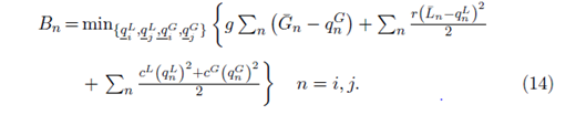
The second-best planner's solution for abatement, , is the same as the Nash equilibrium that does not recognize dimming (11)
When the dimming effect is ignored, the second-best planner's first-order condition for the global pollutant is similar to (12) but without the benefit share term
Similar to the local pollutant, this gives a dominant strategy solution for each region when dimming is not recognized
Across both regions this results in an aggregate abatement level of the global pollutant equal to .
Recognizing the Dimming Effect
Here we consider the impact of recognizing the dimming effect. We first derive the Nash equilibrium where each region chooses abatement to minimize individual damages, taking as given emissions abatement in the other region. We then consider the first-best solution where a planner that recognizes the dimming effect internalizes all externalities across regions.
Unilateral (Noncooperative) Abatement
Under unilateral policy each region independently chooses abatement levels to maximize their individual net benefit from abatement. As before, we can write the benefit from abatement as avoided damages from pollution. Damages from emissions are determined after abatement, , from the BAU level and . The objective function of region now includes the effect of local pollution on global pollution damage
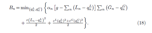
Using aggregate BAU emissions of the two pollutants, the first-order condition with respect to the local pollutant is

The first term is the direct effect of local abatement reducing local damage; the second term is the indirect effect from dimming. It reveals that reducing the local pollutant unilaterally increases the own damages from the global pollutant. The third term is the marginal abatement cost of the local pollutant.
The first-order condition with respect to the global pollutant is

The first term is region 's marginal benefit from abatement and the second term is the corresponding marginal abatement cost. Note that the first-order conditions in (20) depend on three abatement levels due to the interaction of the pollutants. From (20) one derives

From this we see that the important determinant of a region's abatement effort is its benefit share, . Each region abates in proportion to its benefit share, which implies that
Using (22) to eliminate from (19) results in
Each region recognizes that, due to the dimming effect, own abatement levels are complements within the region since . This occurs because increasing abatement exacerbates the marginal damage from .
Next, the two first-order conditions for the local pollutant (19) imply

Given our two-region setting, writing out the two first-order conditions yields
and solving for gives
Equation (26) shows that the local pollutants are strategic complements across regions, with the best-response slope determined by the global benefit share due to the dimming effect: . Using (26) to eliminate in (20) yields (see Appendix A)
Finally, using (23) and (27) solves for the Nash equilibrium of the level of abatement (see Appendix A)
Summing across regions, the aggregate level of abatement at the Nash equilibrium, , is then equal to
Following the same procedure for the local pollutant, using (23) and (29), the Nash level of abatement is
Summing across regions yields the aggregate level of abatement at the Nash equilibrium
Recall that we restrict our attention to interior solutions with positive abatement levels but which are less than BAU emissions, so and for .
The Social Optimum
The socially optimal policy involves a planner that chooses all four abatement levels to minimize the sum of environmental damages and abatement costs across both regions while accounting for the dimming effect

The four first-order conditions are
Using the two first-order conditions in (33) results in
therefore
which implies that if . That is, higher BAU emissions entails greater marginal damage on the last unit, hence requiring more abatement of the local pollutant within a region.
Since the social planner internalizes all the externalities, we obtain the standard Samuelson condition for abatement of the global pollutant. Rearranging (34) yields
Substituting (37) into (33) and rearranging implies
From this one can directly infer the complementary nature of the interacting pollutants which the planner recognizes, i.e., .
Use (38) to eliminate in (34) to obtain the socially optimal level of abatement in each region
Since , the optimal aggregate level of abatement across the two regions is simply . Thus, the optimal level of abatement in each region, which can be found by directly substituting (39) into (38), is
This concludes the derivation of the Nash and socially optimal abatement levels when the policymaker takes account of the dimming effect.
Main Results
After having derived the relevant abatement levels with and without consideration of the dimming effect, we are now in a position to make direct policy comparisons. As a point of reference, Table 1 summarizes the abatement quantities, as derived in the previous section, from which we will be able to obtain our key results. In what follows, we restrict the policy comparisons to interior solutions, reflecting non-negative abatement levels but which are less than the respective upper bounds in terms of BAU emissions. Note that we have identified eight abatement levels for two regions. For interior solutions we then have upper and lower bounds for 16 abatement levels, implying 32 inequalities that need to be satisfied simultaneously. The three parameter restrictions identified in Lemma 1 below are the necessary and sufficient conditions for the existence of all possible interior solutions (proof in Appendix A).
Summary of regional abatement quantities with and without dimming
| Pollutant | Without dimming | With dimming | ||
|---|---|---|---|---|
| Nash () | Second-best () | Nash () | First-best () | |
Notes: and ; see also Lemma 1.
where and .
The first comparison we make concerns the case of unilateral abatement in each region. This situation involves the Nash abatement levels of both the local and global pollutant with dimming () and without recognizing dimming . Propositions 1 and 2 summarize the comparison for the local and global pollutant, respectively. The proofs of all propositions are in Appendix B.
The Nash equilibrium ignoring the dimming effect results in more abatement relative to the level of abatement at the Nash equilibrium that acknowledges the dimming effect
The Nash equilibrium ignoring the dimming effect results in more abatement relative to the level of abatement at the Nash equilibrium that acknowledges the dimming effect
Propositions 1 and 2 indicate that Nash equilibrium abatement of both pollutants is greater when the dimming effect is ignored. Ignoring the dimming effect results in dominant strategy solutions for both pollutants [see in (11) and in (17)], hence there is no strategic response from a change in abatement of either pollutant in the other regions. Neither the benefit externality (via ) nor the dimming effect are internalized in the Nash equilibrium that ignores dimming. Therefore, each region doing the best that they can will choose more abatement of both pollutants than they would if they acted in their own self-interest, but recognize dimming.
Previously in the section "Unilateral (Noncooperative) Abatement" we have shown that recognizing dimming involves strategic interaction for both pollutants across both regions in the Nash equilibrium. Each region that recognizes dimming will choose less abatement of the local pollutant, since this increases their own damage for a given level of the global pollutant. Furthermore, recognizing dimming means acknowledging the complementarity between the pollutants, i.e., from equation (23). Hence, reducing local abatement means reducing global abatement as well. The strategic interaction means that both regions that recognize dimming are responding in the same direction, hence both local and global abatement is less in the Nash equilibrium that recognizes dimming.
The next set of policy comparisons relate to the optimal level of and abatement with the corresponding levels in the second-best outcome which ignores the dimming effect. Propositions 3 and 4 sum up the comparison for the respective pollutants.
The optimal level of abatement recognizing the dimming effect is lower than the second-best level of abatement that ignores the dimming effect
The optimal level of abatement recognizing the dimming effect is lower than the second-best level of abatement that ignores the dimming effect
Propositions 3 and 4 tell us that a planner that does not account for the dimming effect will choose too much abatement of both the local and global pollutant. The planner that recognizes dimming understands the complementary nature of abatement, i.e., following equation (38). However, the planner who does not recognize dimming chooses a dominant strategy for local abatement in (11)] and a dominant strategy for global abatement in (17)]. The first-best planner recognizes that there is too much local abatement (relative to secondbest) since the dimming effect reduces global damage. Given the complementarity, the first-best planner also recognizes that there is also too much global abatement by the planner that does not recognize dimming. A well-intentioned planner who ignores the dimming effect will therefore choose too much abatement of both pollutants across both regions. Thus, even though the global pollutant externality is internalized across regions, the second-best planner does not recognize the global externality created by the dimming effect. The secondbest planner is clearly not internalizing all the externalities from both pollutants across regions when the interacting nature of the pollutants through the dimming effect is ignored.
The final set of policy comparisons concerns the dimming scenario by contrasting abatement at the Nash equilibrium () with the corresponding first-best level of abatement . Propositions 5 and 6 outline the main findings from this comparison for the local and global pollutant, respectively.
When the dimming effect is acknowledged, the firstbest level of abatement, , is higher than the corresponding level of abatement at the Nash equilibrium, , for all benefit shares
When the dimming effect is acknowledged, the first-best level of abatement, , is higher than the corresponding level of abatement at the Nash equilibrium, , for all, withdefined as follows (see Equation (A39))
Proposition 5 indicates that there is too little abatement of the local pollutant at the Nash equilibrium when the dimming effect is recognized. The optimal (first-best) outcome depicts a social planner that acknowledges the dimming effect. Reducing emissions in one region has a negative impact on the other region via the dimming effect that is not internalized at the Nash equilibrium. If a region unilaterally decides to reduce its emissions, the dimming effect becomes stronger, which increases the environmental damage from a given level of emissions.
Proposition 6 shows that there is also too little abatement of the global pollutant at the Nash equilibrium when the dimming effect is recognized, but only as long as the benefit shares are not too different, as defined by a critical threshold value . For similar benefit shares, , Nash abatement of is too low, the standard result from the international environmental agreements literature that does not consider the dimming effect (e.g., Finus and Caparrós, 2015). However, the dimming effect raises a possibility that could not occur in this single pollutant literature. If a region has a sufficiently large share of the benefit from abatement , the optimal outcome would actually imply reducing abatement relative to the Nash equilibrium that recognizes dimming (). The optimum equates marginal abatement cost across the two regions and the first-best planner achieves this by equating with (see Table 1). The large benefit share region reduces abatement since the other region is increasing it, resulting in a cost-effective solution, unlike the Nash equilibrium. The first-best planner always results in a greater level of abatement than at the Nash equilibrium when dimming is recognized (see Table 2). However, the planner's re-allocation of abatement across regions can result in a (very) high benefit share region actually reducing global abatement. This would not occur without the dimming effect. Proposition 5 tells us that optimal abatement is always greater than the Nash equilibrium when dimming is recognized, since the dimming externality is internalized across regions. Furthermore, we know that the optimal planner recognizes the abatement complementarity, i.e., following (38).
Equilibrium abatement quantities and emissions taxes with and without dimming
| Pollutant/ region | Without dimming | With dimming | ||
|---|---|---|---|---|
| Nash () | Second-best () | Nash () | First-best () | |
| 48 | 48 | 21.33 | ||
| 70 | 33.33 | |||
| 70 | 33.33 |
Notes: The outcomes are based on parameter values , and . These values ensure that conditions defined by (41) all hold, ensuring interior equilibrium solutions. Corresponding sulphur and carbon tax rates shown in squared brackets.
Implications for Climate Policy
Now we have derived the optimal and Nash abatement levels of the local and global pollutant with and without accounting for the dimming effect, we can draw some implications for the design of pollution control policy to correct for the cross-regional inefficiencies. In view of the importance of cross-national coordination of abatement efforts, we shall consider a market-based climate policy through a lens of emissions taxation and show how this can be embedded into an international climate agreement to facilitate the coordination process.
Historically, international climate agreements have implemented quantity-based targets. For instance, the Kyoto Protocol required a minimum reduction relative to 1990 emissions levels for Annex I nations. However, the design and implementation of domestic policies that were needed to meet the internationally negotiated abatement requirements were left to the individual member nations. Some literature has recently demonstrated that a carbon tax may be an effective policy instrument for future climate agreements due to many desirable properties. These include negotiating a single price rather than an abatement requirement for each signatory, and tax revenues generated by the agreement that can be rebated to citizens covered by the agreement (McEvoy and McGinty, 2018; Weitzman, 2014). Although our theoretical results are derived in terms of abatement levels, we can straighforwardly relate these to emissions taxes, in particular sulphur and carbon taxes.
Before we go into a more general discussion of emissions taxation in the context of international climate agreements, let us first illustrate some of our key findings intuitively by means of a numerical example. In line with our main approach, base parameters in our numerical exercise were chosen such that it restricts the attention to interior equilibrium solutions, which, we believe, represents the current situation in climate agreements realistically. Table 2 contains the computed abatement levels of and for both regions at the Nash equilibrium with and without acknowledgment of the dimming effect, as well as abatement in the second-best and first-best cases. The corresponding sulphur tax and carbon tax for each distinguished case is given in squared brackets.
Without acknowledging the dimming effect, the only harmonized tax rate across the two regions is the global carbon tax in the second-best setting with . When regions take unilateral abatement decisions while ignoring dimming, the carbon tax at the Nash equilibrium is only harmonized for the special case where the regional benefit shares are perfectly symmetric (). In this case, the carbon tax amounts to . If the benefit shares are unequal (), then, as expected, the Nash carbon tax is higher for the region that experiences higher environmental damages and equal to . Looking at the taxes imposed on emissions without consideration of the dimming effect, both the Nash and second-best sulphur tax rates and , respectively) are independent of the regions' benefit shares, ensuring a proportionate reduction in BAU emissions. Hence, the sulphur tax is higher in the region which generates relatively more emissions (in the numerical example this is region , which implements a sulphur tax of
; region 's sulphur tax is ).
When the dimming effect is accounted for in climate policy, then the Nash equilibrium sulphur tax in region is lower compared to the Nash sulphur tax absent dimming (i.e., ) and is, moreover, decreasing in the benefit share due to the dimming effect (i.e., ). The first-best sulphur tax is lower than its second-best counterpart and independent of the regions' benefit share (i.e., for region for region ). This is due to the internalization of the dimming externality. It is important to note that the optimal sulphur tax is not harmonized across the two regions . This is because individual regions must balance the local damage resulting from emissions with the dimming effect. That is, the optimal sulphur tax is region-specific because the local marginal damage differs on the last unit when emissions vary regionally. In contrast, looking at emissions, the optimal carbon tax is uniform across the two regions but lower than the second-best tax rate . Thus, the optimal sulphur tax is heterogeneous across regions and below the harmonized optimal carbon tax . This means that marginal abatement costs are not equalized across the two pollutants in equilibrium.
Proposition 6 tells us that recognizing dimming can result in a high benefit region actually reducing abatement at the first-best solution compared to the Nash equilibrium that recognizes dimming. Table 2 shows that Nash CO2 abatement is 44 for all possible distributions of the benefit shares; the first-best level of total abatement is 66.67, with each region abating and facing the same marginal cost of the last unit. However, suppose , exceeding the critical value , and , then and . In this case, region would reduce global abatement at the first-best, while region increases abatement to , which equates the marginal abatement cost of the last unit.
This would not happen without the dimming effect from interacting pollutants. Since , the first-best solution would always imply increasing abatement from the Nash equilibrium.
What lessons can be derived from this exercise for the formation of climate policy? Current climate policy disregards the dimming effect, which corresponds to the second-best case that we have identified above. Given our two-region model, the global uniform carbon tax under a multilateral climate agreement would in fact be set too high relative to the first-best uniform carbon tax. The same is true for the second-best sulphur tax rates. The second-best scenario is characterized by the internalization of the global externality from emissions but not the externality that arises from the global dimming effect. In contrast, in the first-best scenario, the optimal tax policy internalizes both externalities simultaneously. Since and abatement are complements, the optimal tax levels are below the tax rates that would be set in a second-best setting where the dimming effect is not accounted for.
More generally, and linking back to some of our formal Propositions derived in the section "Main Results", the first-best outcome is being established with a climate policy that accounts for the global dimming effect. This would correspond to a climate agreement that not only includes the abatement levels of the local pollutant but also their interaction with the global pollutant. Propositions 5 and 6 stipulate how abatement decisions are affected when the dimming effect is recognized. In the presence of dimming, Proposition 5 tells us that too little abatement of the local pollutant occurs at the Nash equilibrium relative to the first-best abatement levels. This implies that, absent any global climate agreement, a single region's sulphur tax is too low. Furthermore, the sulphur taxes at the Nash equilibrium will differ across regions, with the tax rate decreasing in BAU emissions of .
The Nash equilibrium carbon taxes will differ across regions, other than the knife-edge case where benefit shares are equal. Otherwise the region which has a higher benefit share will have a higher carbon tax. With respect to the global pollutant, Proposition 6 suggests that, if dimming is recognized, the Nash carbon tax rates are higher than the first-best levels up to some critical level of the benefit share ( in the numerical example). If then the carbon tax will be higher at the first-best, but if , then the first-best could actually be a reduction in the domestic carbon tax to equate with the global carbon tax. The carbon tax in the low-benefit region would necessarily increase dramatically until it is equated across regions.
Currently existing climate policy does not acknowledge the dimming effect. Without an agreement, abatement of both the local and global pollutants are dominant strategies, since neither externality is internalized at the Nash equilibrium. Each region abates a constant proportion of the local pollutant. Abatement of the global pollutant in a given region, and hence the carbon tax, is strictly increasing in the region's benefit share. Without dimming, sulphur taxes and carbon taxes are higher than at the Nash equilibrium that recognizes dimming. Therefore, ignorance of the dimming effect can, in fact, be welfare improving absent a global agreement on emissions.
Furthermore, without recognition of the dimming effect, abatement of the local pollutant in the second-best outcome is the same as the level of abatement at the corresponding Nash equilibrium. This implies that a region's second-best sulphur taxes are equivalent to the tax at the Nash equilibrium, which is a region's dominant strategy solution. These abatement levels are constant proportions of BAU emissions, and there is no link in a global climate agreement between sulphur and carbon taxes in a second-best world. These findings complement D'Autome et al. (2016), who show that locally differentiated taxes could go hand-in-hand with a global carbon tax even in a second-best setting. On the other hand, van der Ploeg and de Zeeuw (2016) find alternative pricing arrangements, depending on the nature of cooperation between countries in a North-South context with climate tipping points. They show in a dynamic model that carbon taxes tend to converge (diverge) in the cooperative (noncooperative) scenario. In other words, cooperation exhibits more effective coordination, which is conducive to establishing a uniform carbon pricing mechanism. In contrast, carbon prices become more differentiated when countries act noncooperatively in coordinating abatement actions.
The 1997 Kyoto Protocol had ambitious abatement requirements (for Annex I nations) but did not acknowledge the dimming effect. This corresponds to our second-best planner where the agreement was narrow in membership but deep in terms of abatement. The 2015 Paris Accord has Nationally Determined Contributions (NDCs) for abatement. This agreement is broad in terms of membership, but shallow in terms of abatement levels if the NDCs are what each nation would do in the absence of an agreement. The Paris Accord is arguably closer to our case of the Nash equilibrium that does not recognize dimming. There is no single price of carbon under the Paris Accord and each nation chooses their own price to meet their NDC.
Our results also relate to the conventional wisdom regarding the EKC for both local and global pollutants. Currently these EKC's are "de-coupled" in the sense that local pollution has no impact on global damages, that is, the dimming effect is ignored. The local pollutant EKC has a turning point, suggesting a reduction as nations gain sufficient income. Recognizing the dimming effect would then imply an upward shift in the global EKC as income increases. Recognizing dimming would link the two EKCs for both the noncooperative outcome as well as for international climate agreements.
Conclusions
International coordination of climate change mitigation efforts, and the corresponding negotiations and fixing of emissions reduction targets, are often centered around reducing carbon dioxide () emissions without taking into account as to how this global pollutant interacts with local (regional) pollutants, such as, for instance, sulphur dioxide () and nitrogen oxide (). This paper contributes to the literature on multipollutant interactions by studying how the interdependence between and affects the corresponding abatement decisions of regions in the presence of the global dimming effect. The dimming effect refers to the impact of abatement on the environmental damage derived from emissions. Acknowledging the dimming effect gives rise to two interrelated externalities with spatial spillovers which shape the (optimal) abatement decisions of individual regions.
In a simple two-region model, this paper examines and derives abatement of and in the situation where regions coordinate abatement actions non-cooperatively (à la Nash) and cooperatively. Given these policy scenarios, we further analyze abatement with and without acknowledging the dimming effect. The optimal outcome represents the case which acknowledges dimming and where regions coordinate abatement of and simultaneously in order to minimize environmental damage originating from the joint production of these interactive pollutants. Three sets of results are derived.
First, in the non-cooperative scenario where both regions unilaterally minimize the aggregate environmental damage from and , Nash equilibrium abatement is lower with dimming compared to abatement at the Nash equilibrium without acknowledgement of the dimming effect. Second, the optimal level of both pollutants is lower relative to the respective second-best abatement levels which ignore the dimming effect. In other words, there is over-abatement when the dimming effect is not accounted for in coordinating abatement actions. Third, in the presence of dimming, comparing the Nash level of abatement with the optimal level reveals under-abatement at the Nash equilibrium. This result is unambiguous for the local pollutant but holds for the global pollutant under the condition that the regions are not too heterogeneous in terms of the respective benefits they derive from reducing emissions.
These results have important implications for policymakers facing the challenge of reducing local air pollution while simultaneously mitigating global climate change. The results signify that policymaking not only involves how countries unilaterally control the pollution and abatement activities concerning and , but also how this translates into multilateral pollution control efforts. We illustrate such a translation in the context of international climate agreements and show that a firstbest climate agreement involves a uniform tax on the global pollutant () but allows taxes on the local pollutant () to vary across regions. A market-based mechanism like emissions taxation would allow an international climate agreement to reflect the interactive nature between and optimally.
Our theoretical model is an initial attempt to investigate the implications of reducing local pollution on the strategic incentives and impacts of greenhouse gas emissions. Our model involves several simplifying assumptions that impose limitations. First, we assume constant marginal damage from the global pollutant. Much of the literature on international climate agreements assumes convex damages and hence declining marginal benefit from abatement (Barrett, 1994; Finus and Caparrós, 2015). A second simplification is that we have assumed that the dimming effect from reducing local pollution is symmetric across regions. The recent literature on intentional climate engineering to limit the impact of greenhouse gases suggests that the cooling effects may have a disparate impact across regions (Keith, 2000; Moreno-Cruz, 2015). Indeed, Sandler (2018) notes that nations may use marine cloud brightening to provide a local dimming effect generating cooling that is not global in scope. While our focus is on the private benefits from reducing local pollution and the resulting increase in global pollution damage, future research is needed to understand the additional implications of intentional dimming. Future research can extend our model on the relationship between local and global pollutants by considering more complicated and realistic assumptions that may lead to richer and perhaps even different strategic interactions.
Appendix A: Existence of Interior Abatement Solutions
To ensure the existence of interior emissions abatement levels, the following three parameter restrictions need to be satisfied (see Lemma 1):
Below we prove the existence of the interior abatement solutions. We first do this with respect to emissions abatement under the non-dimming case, followed by the derivations for the dimming scenario. For reasons of expositional clarity, and following the terminology in the main text, wherever possible we make use of the terms and defined by and .
Non-Dimming Restrictions
in (11)
An interior solution is always ensured since and all parameters are strictly positive. Therefore, a constant proportion of BAU emissions is abated in each region.
in (17) to be an interior solution requires
otherwise there are no emissions in the second-best outcome which ignores the dimming effect. We therefore require
which is the right-hand side of for .
in (13) to be an interior solution requires
or
Since this inequality is ensured by the binding restriction (A3).
Equations (4)-(6) detail how the marginal damage from the global pollutant is strictly positive for all levels of local abatement. This requires , which is the LHS of . Taken together with (A3), this results in the single parameter restriction , which ensures that all eight no-dimming abatement levels are interior solutions. is both a necessary and sufficient condition
must hold for both regions, so it is binding for the smaller BAU region and slack for the larger BAU region. In what follows, we have multiple restrictions in terms of overall (and not region-specific, ), meaning that we can add across both regions to obtain a combined
The combined is a necessary but not a sufficient condition. It allows for all possible combinations of and for a given . Whichever is smaller will be binding, and the average is only binding if .
Dimming Restrictions
The dimming restrictions are more complicated than the non-dimming restrictions, so we write the dimming abatement quantities in (30) and (40) in terms of non-dimming abatement quantities plus an additional term. This is what we implement below.
in (30) can be written as
Using (A1) above this becomes
Below we will show that we require two more parameter restrictions for the possibility of an interior equilibrium. These are and , which together ensure the term in squared brackets . This term must be smaller in magnitude than for .
in (40) is
Using (A1), rewrite this in terms of the non-dimming level
Given and , the dimming term is negative, hence the magnitude must be less than for .
in (28)
which is positive given and .
in (39)
which is positive given and .
Combined Restrictions
Combining the abatement levels across regions results in a necessary but not sufficient condition. If the necessary condition is not satisfied, then an interior solution is not possible. The combined restrictions would be both necessary and sufficient if regions are identical, i.e., .
in (39) is an interior solution when
Combining this condition as above for results in , where
since . So we have the necessary condition for an interior solution for
Using (A16) and (A7), we can now show that is not possible at an interior equilibrium. Substituting the expressions and into (A16i) implies
Solving the left inequality for results in
Comparing (A18) with the combined condition in (A7) implies
This inequality cannot hold, since . Therefore, and , which from (A16ii) implies .
in (28) is an interior solution for
Combining this condition for results in
since and . Restrictions and ensure that is strictly positive and below the upper bound, .
in (30). For an interior solution
then adding this up for regions results in
since and . The combined dimming term is negative given and imply and .
Lastly, in (40) is an interior solution when
Combining across regions gives
Again, the dimming term is strictly negative given and , hence the lower bound is the relevant one.
Appendix B: Proposition Proofs
Proposition 1
Proof. From (A9)
The difference between and is driven by the dimming term , which is strictly negative given parameter restrictions and . Therefore, .
Proposition 2
Proof. From (13) and (28) we have
Using the definition results in
Then using the definition implies
which always holds given Combined (A7). Therefore, .
Proposition 3
Proof. From (A11)
The difference between and is the dimming term , which is strictly negative given parameter restrictions and . Therefore, .
Proposition 4
Proof. From (17) and (39) we have
Using the definition and this becomes
(A32)
which always holds given Combined (A7). Therefore, .
Proposition 5
Proof. Using (A9) and (A11)
Since from (A1) we have
Restrictions and imply
The right-hand side is strictly positive given and . If the righthand side then for all
The lowerbound of the right-hand side term is 2 , hence, given , this holds for all and .
Proposition 6
Proof. Using (A12) and (A13)
The right-hand side is strictly positive given and . Further,
Given and , the lower bound of is 2 . However, the upper bound is strictly less than since
implying is possible. Therefore, for all , where is defined by
References
Corresponding author
We thank Daniel Heyen, Corrado Di Maria and Danny Campbell for valuable comments on earlier drafts, as well as two anonymous referees for constructive comments and suggestions. We also thank Dominique Thronicker for input in the early stages of this research. The usual caveat applies.
Our paper details the relationship between two types of pollutants and recognizes that eliminating may exacerbate the damage from due to the dimming effect. But there are many other forms of using particulate matter to "dim" the atmosphere, a process more generally known as geoengineering (Moreno-Cruz, 2015; Reynolds, 2019). Although our paper in itself is not about geoengineering, that is the deliberate manipulation of the environment at such a large scale that it may curb or reduce the risks associated with anthropogenic climate change (Keith, 2000), solar radiation management (SRM) as one form of engineering the climate system could reinforce this negative correlation. This could potentially lead to less co-benefits or higher environmental damages. For some key contributions on geoengineering and SRM in the environmental economics realm see Barrett (2008), Moreno-Cruz (2010, 2015), Goeschl et al. (2013), Heyen et al. (2015), Heutel et al. (2018), Emmerling and Tavoni (2018), Heyen et al. (2019), Reynolds (2019), and McEvoy et al. (2023).
To keep the model analytically tractable and as simple as possible, we employ a linear rather than a convex specification of the global damage function, as the latter would generate a nonlinear system of four first-order conditions from which no closed-form solutions to the equilibrium abatement levels can be obtained. However, as we will see in the section "Main Results", clear results can be derived by directly comparing the relevant first-order conditions. Linear damage functions are commonly assumed in the literature (Nordhaus, 2015; see Lessmann et al. (2015) for a comparison of integrated assessment models).
We thank an anonymous referee for making the important point that the physical units are not the same and that we implicitly assume a converting factor via our choice of units.
It is natural to interpret our two-region world as a North-South model where a region with a higher GDP per capita is willing and able to pay more for abatement due to a higher value of avoided damages from extreme weather events. Another possible interpretation is that each region has the same benefit from avoided global damages. This would imply that the benefit share is the global population share for each region. For a discussion on asymmetric benefit shares, see McGinty (2007) and Finus and Caparrós (2015).

