


Border carbon adjustments (BCAs) have been suggested as a measure to reduce carbon leakage in the presence of unilateral climate policies and/or to enforce cooperative climate agreements. In an intra-industry trade model, this paper studies whether and under which conditions a sequence of escalating threats of implementing BCA-measures could be successful in enforcing a fully cooperative agreement. We start from a situation where moving from non-cooperative production-based carbon taxes to a socially optimal tax is not attractive to the environmentally less concerned country. We then test whether the threat of imposing BCA-measures, in the form of import tariffs or, additionally, supplemented by export rebates, will enforce cooperation. We show that import tariffs are the least distortionary policy instrument but the weakest threat, and import tariffs with a full export rebate is the most distortionary instrument if implemented but the most effective threat to enforce cooperation. In an escalating penalty game, we determine the subgameperfect equilibrium path along which threats are deterrent and credible. We show that BCA-measures help to enforce cooperation, reduce global emissions and are welfare improving if they need to be implemented. However, whenever full cooperation would generate the highest global welfare gains, BCAs fail to establish cooperation, a version of the paradox of cooperation, as proposed by Barrett (1994).
Introduction
An effective solution to climate change requires cooperation among all countries in reducing global greenhouse gas emissions. However, strong free-rider incentives constitute a major stumbling block to reach a global agreement. Furthermore, the effectiveness of unilateral actions by some countries is weakened by carbon leakage. One of the channels of carbon leakage is the relocation of the production of firms, in particular in emission-intensive trade-exposed industries, to countries with lower environmental standards. As a result, firms operating in countries with a stricter climate policy lose market shares in the domestic but also international markets.
In order to address carbon leakage and to incentivise higher carbon taxes globally, border carbon adjustments (BCAs) have been proposed (e.g., Elliott et al., 2010; Helm et al., 2012; Stiglitz, 2006). BCAs are trade measures complementing climate policies. (i) BCAs on imports levy a carbon tariff on imports from countries with lower environmental standards; (ii) BCAs on exports provide a rebate on exports to firms faced with higher environmental standards; (iii) BCAs on imports and exports, which are sometimes called full BCAs. The purpose of import tariffs and export rebates is to create an equal playing field - they reduce the disadvantage of firms located in countries with higher environmental standards.
Trade measures to support environmental policies can be defended, based on economic efficiency, as a second-best solution, correcting distortions resulting from the failure of internalizing damages of transboundary pollution (Copeland, 1996; Helm et al., 2012; Hoel, 1996; Markusen, 1975; Stiglitz, 2006). In the absence of global action, Markusen (1975) shows that, from a purely national perspective, the optimal combination of policies is a Pigouvian tax on domestic production and a tariff on imports. Even in a cooperative setting, Keen and Kotsogiannis (2014) show that some forms of BCAs are required to achieve global Pareto-efficiency.
In this paper, we consider the role of BCAs in enforcing cooperation. We model an escalating penalty game with various forms of BCAs, including import tariffs but also export rebates. We start our analysis with an initial situation in which two governments impose non-cooperatively a production-based carbon tax on their producers (PB-regime). We first show that only if the individual evaluation of environmental damages in the two countries is similar will both countries be better off under full cooperation (FC-regime). We then consider the situation when full cooperation cannot be achieved and ask the question whether and under which conditions the environmentally more concerned country can enforce cooperation through a sequence of escalating threats. We consider three threats which constitute various forms of BCAs: (1) a carbon tariff which fully adjusts the difference between the two national tax levels (BI-threat); (2) a carbon tariff combined with an export rebate where the rebate rate is chosen optimally and therefore may not be a full rebate (BIE-threat); (3) a carbon tariff combined with a full export rebate which implies de facto a unilateral consumption-based tax (BF-threat).
We show under which conditions a weaker punishment is sufficient to establish cooperation, under which conditions threats need to be escalated, and under which conditions BCAs are not effective at all in establishing cooperation. We show that BCAs can generally be global welfare distorting, even though in equilibrium they are not. Either
BCAs are deterrent enough and establish cooperation or if they are not and therefore implemented, then they are globally welfare improving and reduce global emissions compared to the PB-regime. Hence, we conclude that BCAs are helpful in either fully internalizing a global externality by enforcing full cooperation or partially internalize a global externality if they need to be implemented. Nevertheless, we also confirm the "paradox of cooperation", as derived by Barrett (1994), in our context with trade and BCAs: whenever the global gains from cooperation would be significant, BCAs are not sufficient to enforce cooperation.
The remainder of the paper is organised as follows. In the next section, we relate our paper to the literature. In the section "Model", we present the ingredients of our three-stage model. In the subsequent sections, we analyse stages in reverse order according to backward induction. The last section concludes and discusses possible future research.
Related Literature
There are now quite some papers that focus on quantifying the impact of BCAs on carbon leakage and the competitiveness of trade-exposed emission-intensive industries (e.g., Böhringer et al., 2014, 2015, 2017, 2018; Fischer and Fox, 2012; Larch and Wanner, 2017). The bulk of these papers use numerical simulations, often by employing computable general equilibrium (CGE) models or integrated assessment models (IAMs). Most of these studies conclude that BCAs can effectively mitigate carbon leakage and reduce the output loss of emission intensive industries. However, most of the reduction in total emissions are driven by BCAs on imports, i.e., carbon tariffs. The role of carbon tariffs as trade sanctions in fostering cooperation on climate change has been studied for instance by Irfanoglu et al. (2015) using CGE models and Nordhaus (2015) using IAMs. However, due to the complicated nature of those models, carbon taxes in those countries on which BCAs are
imposed are assumed to be fixed and often set to zero. Only Böhringer et al. (2016) assumes that those countries could react for instance by retaliation, but this is not an equilibrium choice. Moreover, also emission reduction targets in those countries which impose BCAs do not follow from optimality considerations but are assumed exogenously. Thus, these models do not capture endogenous strategic choices of taxes, tariffs and export rebates.
A far smaller literature is of theoretical nature and considers the role of BCAs in a non-cooperative strategic carbon tax competition game with endogenous policy choices. Helm et al. (2012) consider a simple political BCA-game and argue that exporting countries on which carbon tariffs are imposed respond by taxing their exports rather than remaining inactive or retaliate. However, the predicted behaviour of political actors is not based on a micro-foundation of incentives and hence somehow ad hoc. Sanctuary (2018), assuming perfect competition, and Eyland and Zaccour (2014), assuming imperfect competition, show that import tariffs are effective in pushing all countries to adjust their carbon taxes upward. A closely related paper, by Hecht and Peters (2018), confirms that BCAs allow the country which unilaterally imposes these measures to set a higher carbon tax. However, they find that the optimal response of the country on which BCAs are imposed is to adjust its tax downward. The main difference between their model and ours is that in our model, and similar to (Eyland and Zaccour, 2014), BCAs are explicitly modelled as a function of taxes. In addition, when considering export rebates, Hecht and Peters (2018) assume that both import and export adjustments are imposed at the same rate. In our model, this is not the optimal choice of the country imposing BCAs. Moreover, our paper extends the analysis of BCAs to their strategic role in enforcing cooperation, and their effects on global welfare and global emissions.
The role of BCAs for enforcing cooperation is considered in Anouliés (2015) and Baksi and Ray Chaudhuri (2017). Anouliés (2015) concludes that cooperation is not stable without BCAs, where carbon tariffs support the compliance of at least one country. Baksi and Ray Chaudhuri (2017) show that carbon tariffs can be helpful in enforcing compliance in a repeated game through trigger strategies, even though they are not always effective. However, trigger strategies have been criticized for not being robust against renegotiations (Ederington, 2002; Mason et al., 2017; Van Damme, 1989) and both papers do not consider export rebates.
Model
We consider a three-stage game among two countries, , which is solved by backwards induction. In each country there is a representative consumer and firm. Both firms, , produce a homogeneous emission-intensive good , which generates greenhouse gas emissions. Each firm supplies the home and the foreign market.
First Stage
The first stage is a sequential bargaining game comprising several stages which are displayed in Figure 1. In the initial situation, a bilateral non-cooperative production-based tax (PB-regime) is implemented. We assume that country 1 evaluates environmental damages caused by greenhouse gases more than country 2 . This could be due to objective different environmental damages but could also reflect different perceptions about the need to take climate action. Therefore, country 1 makes a sequence of proposals to country 2 to achieve full cooperation as follows:
In stage 0 , country 1 makes a proposal to move to the full cooperative solution (FC-regime) which is socially optimal. If country 2 accepts, the game ends at node 2 with 'Full Cooperation'. If country 2 does not accept, it responds with 'No Cooperation'. Country 1 could give up and the game ends at node 3, which is identical with the initial situation.
In stage I, if country 1 does not give up, it threats to implement unilaterally the BI-regime (a BCA-regime with only import tariffs) in order enforce full cooperation solution. Country 2 could give in to this threat if the FC-regime is preferred over the implementation of the BI-regime and the game ends at node 4 or the game moves on along the branch 'No Cooperation' to stage II.
In stage II, country 1 either gives in and implements the BIregime and the game ends at node 5 or escalates the threat to the BIE-regime, which implies that the unilateral import tariff is supplemented with an optimal export rebate. Country 2 can either give in to the BIE-threat and cooperate in which case we end up at node 6 or it refuses and the game proceeds to stage III.
In stage III, country 1's threat is further escalated with the BFregime, which differs from the BIE-regime in that the export rebate is as a full rebate. The game ends either in node 8 if this threat was deterrent enough or if not, it ends at node 9 with the implementation of the BF -regime.
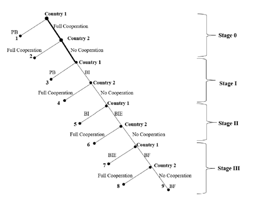
In section "First Stage", we determine the equilibrium path in this game tree. This requires to determine under which conditions threats are deterrent and enforce cooperation but also credible. The sequence of threats is motivated by the assumption that the least globally distortionary instrument should be used first as a threat and only if this does not work, escalation should progress. Moreover, note that whereas import tariffs appear less controversially regarding the compatibility with WTO-regulations, doubts have been raised whether this is also true regarding export rebates (Fontagné and Schubert, 2023; Mehling et al., 2019). We provide further arguments about the sequence of escalation and also discuss alternative assumptions in section "First Stage".
Second Stage
The second stage determines the equilibrium policy levels in both countries for the five policy regimes which are displayed in Table 1. For a given policy regime, policy levels are chosen simultaneously and are based on the following welfare function in countries 1 and 2 :
where is the consumer surplus in country which depends on the total supply to market where is the supply of firm 1 and the supply of firm 2 to market is the producer surplus, which is the total profit of firm based in country from its sale to both markets. is the tax revenue of country imposed on the production of its firm for market and such that are individual damages from global greenhouse gas emissions released in the production of good . Global damages from emissions are where due to the normalisation of the emission-output coefficient which is set to 1 . Hence, global emissions are equal to total production, which is equal to total consumption. For the damage function in countries 1 and 2 , we assume
with a damage parameter, reflecting global marginal damages. We allow for the possibility that countries perceive or evaluate global damages from emissions differently. We assume . That is, country 1 is at least as concerned as country 2 about environmental damages and usually more whenever is strictly larger than The other terms in the welfare function of country 1 in Eq. (1) are introduced in the course of the subsequent discussion of the different policy regimes, as they are only relevant under the three non-cooperative BCA-regimes.
Table 1 gives an overview of equilibrium and effective taxes under the five policy regimes and Appendix A provides detailed calculations. Equilibrium taxes are those taxes which are chosen in country 1 and country 2, respectively. Effective taxes are derived from equilibrium taxes and are those taxes which a firm de facto faces on its sales to markets 1 and 2 (and which are relevant for its optimal output choice). Effective taxes take it account which country imposes the tax and takes import tariffs and export rebates into account. The details will become clear when we discuss the various regimes.
The fully cooperative regime (FC-regime), assumes that both countries jointly maximise the aggregate welfare in both countries with respect to a uniform , ignoring the and term in Eq. (1). Equilibrium and effective taxes are the same and are denoted by . See Appendix A. 1 for details.
Effective and equilibrium carbon taxes under cooperative and noncooperative policy regimes.
| Effective taxes | FC | PB | BI | BIE | BF | |
| Market 1 | ||||||
| Market 2 Equilibrium taxes | BF | |||||
The cooperative regime is contrasted with four non-cooperative regimes.
First, in the production-based regime (PB-regime), each government imposes a carbon tax on the production of its home firm. Hence, the effective tax which each firm faces in both markets is equal to the equilibrium tax imposed by its home country. We denote the corresponding equilibrium taxes by and . As it is apparent from Appendix A.2, if , i.e., the environmentally more concerned country 1 imposes a higher production-based tax.
Second, in the BCA on imports regime (BI-regime), additionally to a production-based tax, country 1 imposes a tariff on imports from country 2 . Thus, firm 1 faces the effective tax as under the PB-regime. Also firm 2 faces on its supply to country 2 as above; however, the effective tax of firm on its exports to country 1 is now given by with the equilibrium adjustment rate on imports. Country 1 is only allowed to impose a tariff provided , with the border tax adjustment rate on imports (Eyland and Zaccour, 2012). That is, under the BI-regime, the term is additionally included in country 1 's welfare function with if , otherwise . We set for two reasons. Any value of above 1 would be illegal under the rules of the WTO. Additionally, given the opportunity of using carbon tariffs, any value of smaller than 1 would not be optimal for country implies that both firms face the same effective carbon tax on their supply to market 1 which is reflected in Table 1. Therefore, BCAs on imports always constitute a "full adjustment" on imports where equilibrium taxes are given by and and . See Appendix A. 3 for details.
Third, in the BCA on imports and optimal export rebate regime (BIE-regime), country 1 supplements its production-based tax and carbon tariff on imports with a rebate on its firm's exports to country 2. We assume that the export adjustment/rebate rate is chosen optimally by government 1 , i.e., , which is not necessarily 1 . Compared to the BI-regime, the effective tax on exports of firm 1 to country , is now given by provided , with the optimal border carbon tax adjustment rate on exports, or, equivalently, the optimal export rebate rate. According to the WTO-rule of non-discrimination, must hold. Generally speaking, the optimal can be positive or negative and can be smaller or larger than 1 . Later, we clarify the range of . At this stage it suffices to point out that it is neither obvious that is chosen such that (full rebate) nor such that (full adjustment) because subsidising exports is costly. Under the BIE-regime, the term is additionally included in country 1 's welfare function with if and , otherwise . Equilibrium taxes and as well as follows from the simultaneous individual maximisation of countries' welfare functions. See Appendix A. 4 for details.
Fourth, the BCA on imports and full export rebate regime (BFregime) is similar to the BIE-regime, except that the rebate rate on exports is not chosen optimally but set to one, i.e., . Hence, firm 1 faces effective tax on its exports and the WTO-rule requires . Equilibrium taxes are given by and . See Appendix A. 5 for details.
Third Stage
Both firms, , compete in outputs in a Cournot-fashion. The inverse demand function in market is given by:
where is the market price in market and parameter is the chock-off price. Total consumption in country is where and are the outputs supplied by firms 1 and 2 to market , respectively. We assume identical firms with a linear production cost function, i.e., , with indicating the location of firm and the market for which the good is produced. Markets
are segmented. That is, firms make separate quantity decisions for the home and the foreign market. The profits of firms obtained in markets 1 and 2 are given by:
where is the effective carbon tax which firm 1 (2) faces on its supply to market 1 and is the effective carbon tax which firm 1 (2) faces on its supply to market and are the total quantities supplied to market 1 and market 2 , respectively.
The simultaneous maximisation of profits obtained in market 1 and market 2 by both firms gives the Nash equilibrium quantities supplied by firms 1 and
with , which we interpret as a market size parameter and/or a parameter which measures the benefits from production and consumption. Accordingly, profits of each firm are given by the sum of profits obtained in market 1 and market 2 :
Hence, effective taxes affect outputs and outputs affect profits of firms.
Third Stage: Results
In this section, we have a closer look at the effect of taxes on equilibrium output levels. These effects are straightforward in the fully cooperative regime with a uniform tax. All output levels for each market are the same. Increasing the tax gradually lowers all outputs uniformly, decreases profits and consumer surplus uniformly, increases tax revenues and decreases damages uniformly, even though, country 1 benefits more than country 2 from lower damages as long as .
In the non-cooperative policy regimes, taxes in country 1 and country 2 will be generally different and also the effects of taxes on outputs.
Under the PB-regime, the standard effect holds: the production of each firm decreases in its domestic tax while it increases in the foreign tax. This encourages governments to adjust taxes downward in order shift profits from abroad to home.
With an import tariff, which is part of all three BCA-regimes (BI-, BIE- and BF-regime), country 1 fully controls the output supplied to its home market. Therefore, all outputs produced for market 1 are negatively affected by tax and are independent of tax . Thus, profits in market 1 are the same for both firms, though profits in market 2 are still lower for firm 1 than firm 2 (because by assumption under these regimes).
If a carbon tariff is supplemented by an export rebate under the BIE- and BF-regime, profits of firm 1 in market 2 are better protected. Export rebates are a step towards levelling the playing field, but because of the WTO-constraint , profits of firm 1 will usually still be lower than of firm 2 in market 2 . Because the effective tax of firm 1 on exports is lower than the equilibrium tax rate, , high equilibrium taxes may not necessarily signal low exports. If , which is possible under the BIE-regime, increasing taxes in country 1 increases exports. If which is the case under BIE-regime, exports of firm to market 2 are independent of taxes in country 2 .
One motivation of BCAs is the possibility of reducing global emissions. How effective taxes are in reducing global emission is considered in the following result.
(The effect of non-cooperative carbon taxes global emissions).
Consider stage 3 in which firms choose their equilibrium output levels which determine total emissions.
- (1) Global emissions decrease in both taxes under the PB-regime:
(2) The carbon tax of country 1 has the largest impact on reducing global emissions under the BI-regime:
(i) if ,
(ii) if , and
(iii) if
wheredenotes the rebate rate which is chosen in stage 2 of the game optimally under the BIE-regime and isunder the BF-regime.
(3) The carbon tax of country 2 has a lower impact on reducing global emissions under the BCA-regimes than under the PB-regime:.
Proof. Follows from inserting the effective taxes in Table 1 into Eqs. (7) and (8) and differentiating total equilibrium output with respect to taxes, recalling that we assume a constant emission-output ratio equal to 1 .
Under the PB-regime, the emission taxes of both governments have the same impact on reducing global emissions. Moving from the PBto the BI-regime, the emission tax in country 1 has a stronger impact on reducing global emissions as it now controls not only its domestic production but also imports. Adding export rebates may partially (if ) or completely (if ) offset the effect of taxes in country 1 on reducing global emissions. In fact, for , the effect of taxes on reducing global emissions is even lower than under the PB-regime and for global emissions even increase under the BIE-regime. Hence, supplementing carbon tariffs with export rebates reduces the environmental effectiveness of taxes in country 1 , even though it may reduce leakage effects caused by country 2 and may also improve the welfare position of country 1 . In contrast, BCA -measures generally weaken the impact of country 2's tax on global emissions. Thus, the effects of BCAs in reducing global emissions is not as straightforward as commonly believed. In order to have the full picture, we need to consider equilibrium taxes, import tariffs and export rebates rates. Nevertheless, the result already indicates that among the BCA-measures the BI-regime is the most effective in reducing global emissions, export rebates may reduce the leakage effect in country 2 further, but may not be as effective as import tariffs in reducing global emissions.
Second Stage
In the second stage, governments choose their climate policy level cooperatively or non-cooperatively. In Appendix A, we derive equilibrium taxes under the full cooperative regime (FC-regime) and the four noncooperative regimes (PB-, BI-, BIE- and BF-regime), including the equilibrium export rebate rate under BIE-regime. We establish existence and uniqueness of equilibria. We also derive what we call border carbon adjustment constraints (BCA-constraints) and non-negativity constraints (NN-constraints) that impose conditions on the parameters of our model. BCA-constraints ensure that equilibrium taxes in country 1 are higher than in country 2 in accordance with the fundamental assumption under the BCA-regimes. Such conditions can be expressed in terms of to be smaller than some threshold with and . We recall that is a measure of the market size in our model, or, a proxy of the net benefits of production and consumption whereas is the parameter that evaluates individual and global damages. NN-constraints are conditions such that all output levels are positive for equilibrium taxes. They require to be larger than some threshold . Hence, if was too large in relation to (i.e., ), equilibrium taxes are too large and would imply negative outputs. Whenever we conduct a comparison across regimes, we assume the most restrictive BCA- and NN-constraints to hold. See in particular Appendix A.6.
Proposition 2 ranks the Nash equilibrium emission taxes across the different regimes.
(Ranking of equilibrium carbon taxes).Consider stage 2 in which equilibrium taxes are chosen under all regimes and the equilibrium export rebate rate is chosen by country 1 under the BIE-regime.
(i) Equilibrium taxes in country 1 can be ranked as follows:.
(ii) Equilibrium taxes in country 2 can be ranked as follows:.
(iii) Under the BIE-regime, if andifwith.
Proof. See Appendix A.7, including the precise definition of
Proposition 2 clearly shows that country 1 chooses higher equilibrium taxes if BCA -measures are available. BCA -measures protect the profits of its firm and address competitive concerns of high carbon taxes. Moreover, country 1 controls a larger share of global emissions. That is, country 1 can better address carbon leakage. Thus, country 1 is more effective in internalising its environmental damages. Additionally, tariffs provide a source of revenues. Equilibrium taxes with export rebates are higher in country 1 , as the effective tax of firm 1 on its exports are lower due to export rebates.
Country 2 also chooses higher equilibrium taxes under the BCAregimes than under the PB-regime. This may be viewed as positive policy spillovers from unilateral BCA-measures by country 1. Country 2 has an incentive to protect is tax revenues if faced with an import tariff and hence raises taxes compared to the PB-regime. This effect is weakened with export rebates, as country 2 tries to protect the competitiveness of its firm in its home market, but still its equilibrium tax is higher than under the PB-regime.
Under the BIE-regime where country 1 chooses its export rebate optimally, this rebate rate is always positive. It is chosen lower than 1 , i.e., partial adjustment, if country 1 evaluates damages sufficiently compared to the benefits from production and consumption, i.e., . If the environmental concern is of less importance, i.e., , then the optimal export rebate rate is larger than 1, i.e., more than a full rebate. In the special case , the rebate rate is exactly 1 .
Proposition 2 suggest that global emissions generally decrease with import tariffs under the BCA-regimes compared to the PB-regime. However, the effect of adding export rebates to carbon tariffs is a priori ambiguous (as equilibrium taxes are larger than effective taxes). The following result ranks global emission levels across the BCA-regimes.
(Ranking of equilibrium global emissions).Given that in stage 2 equilibrium taxes and export rebates are chosen, equilibrium global emissions rank as follows:
(i) BCA-regimes vs PB-regime:.
(ii) Across the BCA-regimes:
if .
if, implying, under BIEregime andif, implyingunder the BIE-regime, with,.
Proof. See Appendix A.8, including the precise cutoff value of .
All BCA-regimes reduce global emissions compared to the PB-regime but BCAs with export rebates are less effective. Despite exports rebates support the climate policy of country 1 (i.e., they reduce carbon leakage and protect its firm's competitiveness), equilibrium global emissions are higher under the BIE-regime than under the BI-regime. This result confirms the main argument against export rebates. They are less effective in reducing global emissions. Only under the BF -regime with a full rebate it is possible that global emissions could be lower than under the BI-regime, but as we show in Appendix A.8, only if the damage evaluation is very small compared to the benefit evaluation of production and consumption in our model. As Proposition 4 will confirm, these are parameter constellations which are not very interesting as the gains from cooperation are small.
Although studying the effects of BCAs on global emissions is important, given that these measures have been proposed for environmental reasons, we need to investigate their impact on global welfare. From a normative point of view, this is relevant because BCAs do not only affect environmental damages, but also production and consumption.
(Ranking of global equilibrium welfare).Letbe equilibrium global welfare in stage 2 and recalland.
(i) FC-regime vs PB-regime:
Let the potential gains from cooperation be, thendecreases in.
(ii)
-regimes vs
-regime:
if and only if.
if and only if.
if and only if.
withand.
(iii) Across the BCA-regimes:
and.
if , implyingunder BIEregime, and if , implyingunder the BIE-regixme.
Proof. See Appendix A.9, including the precise definition of all threshold values.
Regarding the first part of Proposition 4, axiomatically, global welfare in the social optimum is strictly larger than under any other regime. Moving from non-cooperative production-based taxes to a fully cooperative uniform tax implies that the potential global gain from cooperation decreases in . That is, full cooperation matters if is small, i.e., the damage parameter is large compared to the net benefits from the production and consumption parameter .
The second part of Proposition 4 is visualized in Figure 2. On the vertical axis, we have parameter . On the horizontal axis, we have parameter . The upward sloping straight line 'BCA-C' is the BCA-constraint, implying that only values below this line satisfy the BCA-constraint. The upward sloping straight line 'NN-C', implying that only values above this line satisfy the non-negativity constraint. In the feasible parameter range, global welfare generally increases with BCA-measures compared to the PB-regime. Only if the global gains from cooperation are very small (large values of ) and the asymmetry of environmental damages in the two countries is very large ( is large), which need to occur at the same time, will this not hold. Then the gains to country 1 are smaller than the loss to country 2.
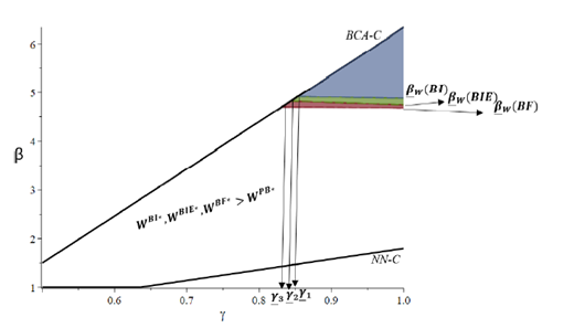
The ranking of thresholds and , as listed in Proposition 4 and Figure 2, suggests that the parameter range in which the BF -regime causes distortions (blue + green + red area) is larger than the parameter range in which the BIE-regime (green + blue area) causes distortions and the parameter range in which the BIEregime causes distortions is larger than the parameter range in which the BI-regime (blue area only) causes distortions. Viewed reversely, there is a larger range of parameter values for which the BI-regime implies a global welfare improvement compared to the PB-regime than this is true for the BIE-regime and the BIE-regime comprises a larger range of parameter values implying a global welfare improvement compared to the PB -regime than this is true for the BF -regime.
According to the third part of Proposition 4, the BI-regime with only import tariffs always implies larger global welfare than the regimes with export rebates (BIE- and BF-regime). Whenever the gains from global cooperation would be large (i.e., is sufficiently small), global welfare is higher under the BIE- than BF-regime ( , such that under BIE-regime according to Proposition 3).
Taken together, when enforcing cooperation through a threat of escalating penalties, it is sensible to proceed along the sequence BI-, BIEand BF -regime in order to minimise the distortions and to maximise global welfare in case those threats would be implemented. This is particular relevant when the potential gains from cooperation are large. This is the guiding principle of the escalating penalty game analysed in the next section.
First Stage
Preliminaries
In this section, we solve the first stage of the game, the escalating penalty game. We ask the question under which conditions can BCAs enforce full cooperation and under which conditions is this not possible. We first derive the equilibrium path in a sequential escalating penalty game. Next, we evaluate equilibria from a global welfare perspective. Finally, we evaluate the robustness of our conclusions for alternative assumptions. As a starting point in order to clarify the basic incentives, we need Proposition 5.
(Individual equilibrium welfare).Consider the first stage of the game.
(i) Country 1 always prefers to move from the
-regime to full cooperation, , but country 2 may be worse off if the evaluation of environmental damages is sufficiently different, ifwith.
(ii) Country 1 is always better off under any of the three
-regimes than under the
-regime, and.
(iii) Country 1 is always better off under the BIE- than BF-regime, .
Proof. See Appendix B.1.
According to result (i), country 1 always has an interest in full cooperation, but this is not true for country 2 if is larger than some threshold . In this case, the portion ( ) of benefits from emission reduction in the form of reduced damages accruing to country 2 is too small to make up for the costs of lower production and consumption due to the internalisation of global damages. In order to render the following analysis interesting, we make the following assumption.
Assumption:
Starting from the PB-regime, country 2 has no incentive to fully cooperate. That is, withas defined in Proposition 5.
Thus, in Figure 1, country 1's proposal "Full Cooperation" is turned down by country 2 in stage 0 . Hence, the equilibrium path in stage 0 is the bold highlighted branch which directly leads to stage I. That is, the interesting part of the game starts in stage I. As country 1 is always better off under any of the BCA-regimes than under the PB-regime according to result (ii) in Proposition 5, it is clear that the game will not end at node 3 in Figure 1, instead country 1 will threat to implement the BI-regime in the next stage of escalation. More generally, in a basic sense, country 1's threat with any unilateral BCA-measure is credible, as it is always better off with implementation than being stuck in the initial situation with a PB-regime. We will explain that credibility entails more than that in Lemma 2.
Note the fact that country 1 is always better off under the BCAregimes than under the PB-regime (Proposition 5), but global welfare does not always increases with BCA-measures (Proposition 4) implies that these cases occur when country 2 is worse off. Given that BCAs are unilateral measures, this is not completely surprising (e.g., Böhringer et al. (2018) and Larch and Wanner (2017)). In fact, after all, BCAmeasures are used as a threat by country 1 to enforce cooperation in our game.
Result (iii) provides an additional argument for the sequence of escalation. The harshest punishment is not necessarily preferred to weaker punishments by country 1 which threats to impose punishment. This relates to choices on (punishment is implemented) and off the equilibrium path (punishment works and is therefore not implemented). In other words, the BF -threat will only be used if the weaker threats have not been able to enforce cooperation and only the harsher BF-threat is capable of this.
The Equilibrium Escalating Penalty Path
For the analysis of the equilibrium path, two features are central. The first feature relates to escalating penalties. We ask the question under which conditions will country 2 accept cooperation for a particular threat and under which conditions will it refuse to cooperate. The relates to the deterrence potential of the threat. The second feature is the credibility of threats. We ask the question whether and under which conditions country 1 has an incentive to escalate penalties. The first question is answered in Lemma 1.
Lemma 1 (The effect of BCAs on the incentive of country 2 to cooperate).
(i) Under the threat of BCAs with tariffs on imports (BI-threat), country 2 is willing to cooperate if.
(ii) Under the threat of BCAs with a tariff on imports and an optimal export rebate (BIE-threat), country 2 is willing to cooperate if.
(iii) Under the threat of BCAs with a tariff on imports and a full export rebate (
-threat), country 2 is willing to cooperate if. wherewith
(iv) None of the threats is successful in enforcing cooperation if.
(v) As the threat escalates from BI to BIE to BF, the welfare of country 2 decreases.
Proof. We have if if if and if . See details in Appendix B.2.
Lemma 1 is illustrated in Figure 3 with the same notation and axis as in Figure 2. The black area denoted by PB is the parameter range in which country 2 would cooperate if faced with the alternative of the PB-regime. We know this would only happen if , which we have ruled out by assumption. The blue area denoted by BI is the parameter range in which the BI-threat enforces cooperation, i.e., condition (i) in Lemma 1 holds, as the implementation of the BIregime implies lower welfare for country 2 than when cooperating. The green area denoted by BIE is the additional parameter space in which cooperation can be enforced with the BIE-threat. That is, condition (ii) in Lemma 1 holds in the blue and green area. The red area is the additional parameter space in which the BF-threat is successful to establish cooperation. Thus, condition (iii) in Lemma 1 comprises the blue, green and red area. Finally, the entire grey area, the 'No Cooperation Region' (region ) is the parameter space in which condition iv in Lemma 1 holds. Thus, Lemma 1 confirms the logic that escalation proceeds along the BI-, BIE- and BF-threat.
The decision of country 2 to cooperate if faced with BCA-threats depends on parameters and . Only if exceeds the threshold , , can cooperation be enforced with a threat. If , even the harshest possible punishment cannot enforce cooperation. That is, whenever the gains from global cooperation would be really large, i.e., is small according to Proposition 4, cooperation cannot be established. This has some resemblance with the paradox of cooperation as established by Barrett (1994), which we will further pursue below.
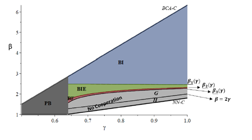
The effect of BCAs on the incentive of country 2 to cooperate and equilibrium outcomes in the escalating penalty game. *BCA-C and NN-C are the BCA-constraint and the non-negativity constraint, respectively.
The effect of BCAs on the incentive of country 2 to cooperate and equilibrium outcomes in the escalating penalty game. *BCA-C and NN-C are the BCA-constraint and the non-negativity constraint, respectively.
The effect of differs across the BCA threats. On the one hand, decreases in (which is hardly visible in Figure 3). That is, the threat becomes more effective if the evaluation of environmental damages of country 2 decreases. As increases, country 2 cares less about damages from emissions and reduces its tax. As a result, the gap between the two taxes increases, the payoff of country 2 decreases and the threat becomes more effective under the BI-regime. On the other hand, and increases in , implying that the area of enforcing cooperation shrinks under the BIE- and BF-regime, as lower damages in country 2 make it less attractive for this country to cooperate. By adding exports rebate, global emissions increase but this effect becomes less damaging to country 2 as increases. Moreover, the optimal export rebate rate of country 1 decreases as increases which reduces the loss that country 2 might incur under the BIE-regime, which in turn reduces the incentive to cooperate.
The second issue that we need to address is the credibility of threats. As noted before, in a basic sense threats are credible because country 1 is always better off under the BCA-regimes than being stuck in the PB-regime. In a more sophisticated sense, a threat by country 1 is only credible if it improves upon the situation without threat. That is, country 1's welfare with full cooperation must be higher than when it does not escalate the threat.
With reference to Figure 1, the following tests need to be conducted. (i) In stage 1, the BI-threat is credible if full cooperation at node 4 generates higher welfare than at node 3 (PB-regime) to country 1 . (ii) In stage 2, the BIE-threat is credible if full cooperation at node 6 generates higher welfare than at node 5 (BI-regime) to country 1. (iii) In stage 3, the credibility of the BF -threat requires that country 1's welfare at node 8 with full cooperation is higher than at 7 (BIE-regime). (iv) And finally, if also the BF-threat has not be deterrent enough, country 1 must implement the BF -regime as it improves its welfare compared to the PB-regime. These tests correspond to the four first points listed in Lemma 2.
Lemma 2 (The credibility of BCA-threats by country 1).
(i) Credibility of BI-threat: country 1 is better off under full cooperation than under the
-regime.
(ii) Credibility of BIE-threat: country 1 is better off under full cooperation than under the
-regime if.
(iii) Credibility of BF-threat: country 1 is better off under full cooperation than under the BIE-regime if.
(iv) Country 1 is better off under all three BCA-regimes than under the PB-regime.
(v) We have: .
Proof. See Appendix B. 3 for (ii), (iii), and (v) and Proposition 5 for (i) and (iv).
The last result in Lemma 2 indicates that full cooperation is particularly attractive to country 1 compared to imposing a unilateral
BCA-regime if the damage parameter is high compared to the parameter of the net benefits from production and consumption , i.e., if is sufficiently small. Even if equipped with the strategic advantage of export rebates in addition to import tariffs, country 1 prefers full cooperation over unilateral trade measures if global cooperation would generate large gains from cooperation, i.e., if is sufficiently small. Thus, the preferences of country 1 are aligned with global welfare.
Finally, we need to combine Lemma 1 and Lemma 2 in order to determine the equilibrium path, i.e., we have to test the compatibility of the conditions of Lemma 1 and Lemma 2. The logic can be illustrated by considering for instance stage III in Figure 1. We note from Lemma 1 that we only proceeded to stage III if . That is, previous attempts to enforce cooperation have failed. Suppose, the BF-threat is successful in establishing cooperation in stage III , i.e., . Hence, together, we have . From Lemma 2, condition iii, we know that the credibility of the BF -threat requires . Therefore, we have to test whether both inequalities and can be satisfied such that cooperation is an equilibrium path and the game terminates at node 8. That is, if the enforcement condition in stage III in Lemma 1 holds, also the corresponding credibility condition in stage III in Lemma 2 holds. Technically, this is done by showing that . The same procedure is applied to stages I and II with similar conclusions which are summarised in Proposition 6.
(Subgame-perfect Nash equilibrium in the escalating penalty game).
(i) Cooperative Region :
If : full cooperation is achieved along the path: Full Cooperation → No Cooperation → BI → Full Cooperation. The game ends at node 4 in stage inFigure 1.
If : full cooperation is achieved along the path: Full Cooperation → No Cooperation → BI → No Cooperation → BIE → Full Cooperation. The game ends at node 6 in stage II in Figure 1.
If : full cooperation is achieved along the path: Full Cooperation → No CooperationNo CooperationBIE → No Cooperation → BF → Full Cooperation. The game ends at node 8 in stage III inFigure 1.
(ii) Non-cooperative Region
Option 1:if, the
-regime is implemented and the game ends at node 9 in stage III in Figure 1.
Option 2:if, the BIE-regime is implemented and the game ends at node 7 and if, the
-regime is implemented and the game ends at node 5 in Figure 1.
Proof. See Appendix B.4.
In the cooperative region, full cooperation is established based on the threat by country 1 to impose BCA -measures. Hence, there are three paths to reach full cooperation. If , country 2 cooperates as a reaction to the BI-threat. This is the blue area in Figure 3. If , the BIE-threat works. This is the green area in Figure 3. And if only the BF-threat works. This is the red area in Figure 3.
In the non-cooperative region, i.e., , none of the threats are successful to enforce full cooperation and the BF -regime is implemented. This is to what we refer as Option 1 in Proposition 6. This is the entire light grey area (region ) in Figure 3. This non-cooperative path results from the assumption that country 1 must commit to its threat provided country 2 does not accept cooperation. Accordingly, the BF -regime is implemented.
However, for the non-cooperative path, also alternative predictions are possible to which we refer as Option 2 in Proposition 6. Option 2 requires two arguments.
First, suppose country 1 cannot implement cooperation even with the harshest possible punishment (BF-regime), then it is not unlikely that country 1 will implement its most preferred BCA -measure. In this case, either the BI - or BIE -regime is implemented; the BF -regime is never chosen. Country 1 always prefers the BIE- over the BF-regime because under the former regime the export rebate rate is chosen optimally whereas under the latter regime it is fixed. Whether country 1 prefers the BIE- over the BI-regime depends on parameter values. Specifically, the non-cooperative parameter space can be divided into two sub-regions. If , country 1 implements the BIEregime (which is region G in Figure 3) and if it implements the BI-regime (which is region H in Figure 3).
Second, in terms of equilibrium paths (not in terms of outcomes) one could argue that we assume a game of full information, which implies that country 1 can anticipate the failure to establish cooperation for . Hence, it will not proceed to stage II if , implementing the BI-regime (i.e., the game ends at node 5 in Figure 1), and will proceed to stage II, but not to stage III if , implementing the BIE-regime (i.e., the game ends node 7 in Figure 1), as spelled out in Proposition 6, Option 2. Option 2 highlights once more that it is not obvious that country 1 always uses the harshest possible threat to enforce cooperation.
Welfare Analysis of Equilibria
In this subsection, we evaluate our results from a normative perspective. We showed in Proposition 4 that BCAs generally raise global welfare compared to the PB-regime. However, there are exceptions. Hence, it is important to understand whether the implementation of the BCAs threats if they were not successful in establishing cooperation are welfare improving.
Corollary 1. If BCAs are implemented because threats are not deterrent enough to establish cooperation (non-cooperative region), they improve global welfare compared to the PB-regime.
Proof. Follows from comparing the threshold levels for which BCAs lead to a global welfare loss in Proposition 4 with the threshold levels for which full cooperation is achieved in Proposition 6 where .
Thus, whenever BCA-measures cannot enforce cooperation, they lead to higher global welfare than in the PB-regime. (That is, all parameter values for which BCAs could lead to a global welfare loss fall in the cooperative region.) It is also worthwhile to recall that country 1 has no incentive to implement BCA-measures along any equilibrium path in the cooperative region because cooperation is preferred to BCA-measures (see Lemma 2).
Another observation which we made above in Proposition 4 was that the potential gains from cooperation, , are large if is small. From Proposition 6 we know that if is sufficiently small, i.e., , none of the BCA-regimes enforce cooperation. Combining both results, we ask the question how successful are BCAs when implemented in the non-cooperative region. In order to answer this question, we employ a relative measure called the closing the gap index (CGI) as suggested by Eyckmans and Finus (2006).
Corollary 2 (BCAs and the CGI).In the non-cooperative region whenis small, i.e., are implemented. , andare decreasing whereas the potential gains from cooperationare increasing when lowering.
Proof. Follows from Propositions 4 and 6 and Appendix B.6.
On the one hand, BCAs close the global welfare gap fully through their strategic role for all , i.e., in the cooperative region. However, if is sufficiently small, , full cooperation cannot be achieved. On the other hand, the lower , the larger would be the global gains from full cooperation but the extent to which BCAs close this gap becomes smaller and smaller. Hence, whenever cooperation would be needed most, BCAs do not enforce cooperation. Moreover, the larger the potential gains from cooperation, the smaller the success of BCAs if they are implemented. As indicated above, this result has some resemblance with 'the paradox of cooperation', a term coined by Barrett (1994) in his seminal paper.
Alternative Assumptions
We have put forward three main arguments to motivate the sequential escalating penalty game with three stages. First, the distortionary global welfare effects of BCAs increases along the latter of escalation with three steps. Therefore, escalation should only be used if needed. Second, export rebates are more controversial than export rebates. Third, country 1 prefers cooperation over the implementation of BCAs along the latter of escalation.
In Proposition 6, we argued that option 2 maybe plausible. That is, if country 1 anticipates that BCAs will be implemented as they are not capable of enforcing cooperation, either the BI- or BIE-regime will be implemented as they are preferred over the BF -regime. That is, the game does not end in stage III (node 9), but either already at the end of stage I (node 5) or at the end of stage II (node 7) in the non-cooperative parameter region. However, if the BF -regime is capable of enforcing cooperation, it will be used by country 1 and we end up in node 8 in stage III of the escalation game. This is certainly the case if only the BF-threat enforces cooperation, but none of the other BCA-regimes can do so, i.e., . In terms of the sequence of escalation, this would not make any difference, all three stages remain in Figure 1, only node 9 could be removed.
This is also the case if we follow the subtle argument that in the cooperative parameter region where the BI-regime enforces cooperation, i.e., , the blue region in Figure 3, also the BIE-regime could enforce cooperation, but if country 1 were to be called upon implementation (off the equilibrium path), it would prefer the BIE- over the BI-regime in this parameter range (see Appendix B.4). This argument maybe viewed as refinement of the credibility of threats. However, given the fact that in the non-cooperative parameter range, country 1 prefers the implementation of the BI- over the BIE-regime in some parameter range (see Option 2 in Proposition 6), all three stages remain in Figure 3.
Irrespective of the arguments above, one may wonder about the outcome of an alternative penalty game with only one stage. That is, country 1 moves first and proposes cooperation, choosing among the three BCA-threats right from the beginning to enforce cooperation.
What would be the outcome of such a game? We provide a short answer here, using again Figure 3, and refer to the reader to Appendix B. 5 for more details, including a graphical representation of the one-shot game.
In order to answer this question, we need to distinguish between the cooperative region and the non-cooperative region as spelled out in Proposition 6.
In the non-cooperative region, it is clear that country 1 would use its most preferred BCA-regime. Accordingly, the conclusion of Option 2 in Proposition 6 holds. If , the BIE-regime is implemented (region G in Figure 3), whereas if the BI-regime is implemented (region H in Figure 3). Hence, there is no difference at all to the sequential game.
In the cooperative region, if (the blue region in Figure 3), any of the three threat options (BI-, BIE- and BF-regime) could establish cooperation, if (the green region in Figure 3) the BIE- and the BF-threat could establish cooperation and if (the red region in Figure 3) only the BF-threat could establish cooperation. Consequently, in a game-theoretic sense, in the first cooperative parameter region (blue region in Figure 3), there are three subgame-perfect equilibria, in the second cooperative region (green region in Figure 3) there are two subgame-perfect equilibria and only in the third cooperative parameter region there a unique equilibrium, even though the outcome is the same (i.e., cooperation is established due to threats) in all cooperative parameter regions as in the sequential game.
We therefore conclude that the sequential escalating penalty game in Figure 1 has the advantage over a game of a simultaneous choice of BCA-threats in that it always delivers a unique equilibrium for each parameter range, even though in terms of outcomes nothing changes. Hence, all qualitative conclusions regarding global welfare derived in the previous subsection still hold. That is, in the cooperative region when BCA-threats enforce full cooperation, the gains from full cooperation over the non-cooperative PB-regime are relatively small and in the non-cooperative region when BCAs fails to establish cooperation and are therefore implemented, even though BCAs are globally welfare improving compared to the PB-regime, the gap between full cooperation and the PB-regime is only closed to a small extent.
Conclusions
The absence of a global agreement to mitigate climate change raises concerns about carbon leakage, which undermines the effectiveness of unilateral actions. Economists and policymakers have suggested BCAs as a measure to address carbon leakage but also to enforce cooperative climate agreements. To this end, we assessed the effectiveness of three forms of BCAs in an intra-industry trade model with two countries, which differ in their perception of environmental damages and which choose their carbon taxes strategically. Our game comprises three stages: countries play an offer/threat response bargaining game in stage 1 with several sub-stages, for each policy regime in stage 1, countries choose their carbon taxes in stage 2 and firms choose their output in stage 3.
We started from a non-cooperative situation of mutual productionbased taxes, which we called the PB-regime. Country 1, which is more concerned about environmental damages would like to move to a cooperative situation of a socially optimal uniform tax with lower global emissions and higher global welfare, but country 2 not: it perceives the benefits from reduced damages and additional tax revenues to be smaller than the loss of producer and consumer surplus. We then analysed whether and under which conditions country 1 can enforce cooperation through threats, which constituted a sequence of escalating penalties. We tested the deterrence potential and the credibility of threats by deriving the subgame-perfect equilibrium path along a sequential offer/threat (country 1) and response (country 2) game. Threats constituted various forms of BCAs.
We considered three designs of BCAs. (a) BCAs on imports, implying that country 1 imposes unilaterally a tariff on imports from country 2 , where this tariff fully adjusts the difference between the carbon taxes in the two countries (BI-regime). (b) BCAs on imports are supplemented by country 1 giving rebates to its firm on its exports to country 2 where the rebate rate is chosen optimally (BIE-regime). (c) The same as b, though the export rebate is not chosen optimally but is a full rebate, which de facto means that country 1 imposes a unilateral consumption-based tax (BF-regime).
We showed that import tariffs and export rebates protect the competitiveness of country 1's firm in the home and the foreign market, respectively. Country 1 can better control global emissions through BCAs as leakage effects are lower. Moreover, country 1 benefits from tariff revenues as they essentially shift tax revenues from country 2 to country 1. However, we also noted that tariffs disadvantage consumers in country 1 and export rebates are costly. This explained among other factors why country 1 may not choose a full export rebate, provided it can choose its rebate optimally. It also explained that if BCAs are successful in enforcing full cooperation, country 1 has no incentive to implement BCAs. If BCAs-threats do not work, then country 1 will be better off with implementing BCAs than being stuck in the PB-regime. Under those conditions global emissions will be lower and global welfare higher than in the PB-regime. In its own interest, country 1 will not implement the most distortionary BCA-regime (and most harmful BCA-regime for country 2), which we showed is the BF-regime, but either the BI- or the BIE-regime. Thus, it emerged from our paper that unilateral BCA measures are helpful in either fully internalizing a global externality by enforcing full cooperation or at least partially internalizing a global externality if they need to be implemented.
Nevertheless, our results also have some resemblance with Barrett's paradox of cooperation (Barrett, 1994). The higher environmental damages are compared to the net benefits from production and consumption, the larger are the potential gains from cooperation, but the harsher must be the threat of punishment in order to enforce cooperation. In particular, when those gains from cooperation are really large, even the harshest punishment is not sufficient to establish cooperation.
In this paper, we considered one aspect of asymmetry among countries, which was the evaluation of environmental damages. One could also look at other aspects, as for instance different carbon intensities across countries (Böhringer et al., 2014; Fischer and Fox, 2012). Another possible extension could be to extend the
-player symmetric agreement formation game considered in Helm and Schmidt (2015) and Al Khourdajie and Finus (2020) to asymmetry. One could analyse possible transfer mechanisms between the two heterogeneous countries along the lines of optimal transfers by Finus and McGinty (2019) considering also trade and BCAs in these models. Finally, one could consider a nonlinear damage function in order to test our qualitative conclusions, even though this requires simulations as analytical results cannot be obtained.
Acknowledgements
We would like to thank Maik Schneider and Ralph Winkler for their helpful comments on an earlier draft. Noha Elboghdadly gratefully acknowledges financial support from the Egyptian Ministry of Higher Education during her PhD studies at the University of Bath.
A Appendix of the section "Third Stage: Results"
In the third stage, the output stage, using Eqs. (5) and (6) in the text, delivers , which guarantees a unique Nash equilibrium in each market (Eichberger, 1993; Friedman, 1986). That is, .
The welfare functions in Eqs. (1) and (2) in the text can be written explicitly as follows:
We define . We recall that is a proxy for the market size or the net benefits of production and consumption, is the global damage parameter and the share parameter of global damages.
Due to lack of space, the subsequent proofs are a sketch; detailed computations are available from the authors upon request.
FC-Regime
Inserting uniform taxes for into (7) in the text, gives equilibrium outputs and . Inserting equilibrium outputs into the aggregate welfare function , differentiating with respect to , yields the following first- and second order conditions:
and . Solving for the socially optimal carbon tax, leads to:
Hence, we have and . In order to have positive production levels (i.e., interior solutions), we impose the non-negativity constraint (NN-constraint) or, using .
Note that this constraint as well as those required under the other regimes are summarised in Table A. 1 in Appendix A.6.
PB-Regime
Inserting effective taxes in Table 1 into Eq. (7) in the text, leads to and . Inserting these outputs into (A.1) and (A.2) and setting , give the following first-order conditions:
and
.
Solving and simultaneously, gives equilibrium taxes:
where the second-order conditions are satisfied because , . Moreover, , which ensures a unique Nash equilibrium. These conditions are also sufficient for the Routh-Hurwitz stability condition to be satisfied (Brander and Spencer, 1985).
Inserting equilibrium taxes into outputs, we obtain equilibrium outputs, equilibrium welfare levels and with and . From equilibrium outputs, the NN-constraint follows. Moreover, we always have for all .
BI-Regime
Inserting the effective taxes in Table 1 into Eq. (7) in the text, leads to and . Inserting these outputs into (A.1) and (A.2) and setting , we obtain and . The first-order conditions are given by:
and .
Solving and simultaneously, gives equilibrium taxes:
where the second derivatives are given by and . Therefore, we have , which ensures a unique and stable equilibrium.
Inserting equilibrium taxes into outputs, it turns out that the most restrictive NN -constraint requires and equilibrium global emissions are given by .
Since the difference between the two equilibrium taxes is ambiguous, we need to impose a BCA-constraint such that . The BCAconstraint requires . Inserting and into welfare functions, gives and .
BIE-Regime
In models with imperfect competition, generally, equilibrium taxes can be positive or negative (in which case they are subsidies). Therefore, the feasible values of the rebate rate depends on the equilibrium taxes in country 1 and country 2. Moreover, we need to consider and .
If . We have where for the maximum allowable rebate rate holds if , while if . If , then . In such cases, the feasible values for is . This is illustrated below.
Inserting effective taxes in Table 1 into Eq. (7), gives equilibrium output levels and . Inserting these outputs into (A.1) and (A.2), gives the welfare function of each country under this regime.
The first-order conditions are given by:
with the last condition being the same as in the BI-regime.
Solving and simultaneously, the Nash equilibrium carbon taxes are given by:
and the optimal export rebate rate is given by:
noting that if . We obtain the following second derivatives: for all for all , and . Hence, second-order conditions hold and guarantees uniqueness.
Inserting equilibrium taxes into outputs, it turns out that the most restrictive NN-constraint requires . Equilibrium global emissions are . We also need to impose a BCA-constraint such that , which leads to . Note that always holds. Inserting and into welfare functions, we obtain and .
BF-Regime
Inserting the effective taxes in Table 1 into Eq. (7) in the text, gives equilibrium output: and . Inserting these outputs into (A.1) and (A.2), gives the welfare function of each country. The first-order conditions are given by
Solving and simultaneously, the equilibrium carbon taxes are given by:
with , and where .
Inserting equilibrium taxes into outputs, the most restrictive NNconstraint requires . Global emissions are given by .
There is no need to impose a BCA-constraint as we always have and with equality if and only if .
Inserting equilibrium taxes into welfare functions, gives and and .
All Regimes
We summarise the conditions that satisfy the NN-constraint and the BCA-constraint under various regimes in the following table. For comparisons across regimes, we use the most restrictive condition, which is summarised under "Feasible Range".
Proof of Proposition 2
(i, ii) The ranking of equilibrium tax levels follows directly from comparing the taxes provided in (A.3) to (A.12), using the NN- and BCAconstraints in the feasible range in Table A.1, i.e. .
(iii) Follows from Appendix A.4, in particular (A.10), where .
Proof of Proposition 3
We compare global emission levels which are given in Appendices A. 2 to A.5. We use the NN- and BCA-constraints in the "Feasible Range" listed in Table A. 1 above.
(i) Comparison with the PB-regime:
if if , and if , where all the above conditions can be shown to violate the NN-constraints. Hence, we have .
(ii) Comparison across the BCA-regimes:
if , which violates the NN-constraints. Thus, we have .
if , which violates the BCA-constraint only if . Thus, if , which already holds for all . Note that if , this implies that and therefore .
if , i.e., if the optimal rebate is less than or equal (larger than) a full rebate, i.e., (>) 1 .
Proof of Proposition 4
Using Appendices from A. 1 to A.5, and upon substitution of equilibrium taxes and outputs in country's welfare function, equilibrium welfare is obtained.
(i) The global welfare gap between the FC- and the PB-regime is .
(ii) Comparison BCA-regimes vs PB-regime
if or . The first condition violates the BCAconstraint for all , while the second condition violates the NN-constraints. Therefore, except if for all .
if or . The first condition violates the BCAconstraint for all , while the second condition is not feasible. Therefore, except if for all .
if or . The first condition violates the BCA-constraint for all , while the second condition violates the NN-constraints. Therefore, except if for all .
We also have for all . Hence, a global welfare loss under any of the BCA-regimes can only occur if .
(iii) Comparison across BCAs regimes:
if or if . The first condition violates the NN-constraints, while the second condition violates the BCA-constraint. Therefore, . In addition, we find that for all values of .
if for all . The first part of the inequality implies that the optimal rebate is larger than a full rebate, i.e., , and the second inequality is satisfied by the BCA-constraint for all . Therefore, if , i.e. if , and if for all .
B Appendix of the section "First Stage"
Proof of Proposition 5
(i) Using Appendix A. 1 and Appendix A.2, we find that for all but if .
(ii) For country if or for all . The first inequality violates the NN-constraints and the second inequality violates the
BCA-constraint. Therefore, we have . Similar results are obtained by comparing the welfare level of country 1 under the PB -regime with the BIE- and BF-regime. That is, if with , and if with , where these conditions hold given our NN- and BCA-constraints.
Proof of Lemma 1
(i) From Appendices A. 1 and A.3: if and/or if . The NN-constraints are not sufficient to guarantee the satisfaction of the first condition; thus it needs to hold. However, this condition violates the BCA-constraint for all . Recall that we consider only the range in which cooperation cannot be achieved under the PB-regime, i.e., from Proposition 5. Therefore, the first condition does not violate the BCAconstraint in our range. The second condition violates the NN-constraint for all . Hence, this condition is not relevant for the parameter range which we consider . As a result, if country 1 imposes the BI-threat, we have if , where for all .
(ii) From Appendices A. 1 and A.4: if (a) and (b) if or for all . We consider the range: . The NN-constraints are not sufficient to guarantee the first condition in (b) and it also does not violate the BCA-constraint. As a result, this condition needs to hold. The second condition in (b) violates the NN-constraints. Therefore, for the range , if country 1 imposes the BIE-threat, if , where for all .
(iii) if (a) and (b) if or for all . We consider the range: . The NN-constraints are not sufficient to guarantee the first condition in (b) and it also does not violate the BCA-constraint.
Thus, this condition needs to hold. The second condition in (b) violates the NN-constraints for all and hence is not relevant here. Therefore, for the range , if country 1 imposes the BF-threat, if , where for all .
In addition, we have for all .
(iv) Along the escalating threat path, the welfare of country 2 decreases as follows:
We find that if and only if . The lower bound condition is satisfied as long as , however, the upper bound condition violates the NN constraint. Therefore, always holds. In addition, we find that for all . Thus, in the region in which country 1 threats with the implementation of the BIE-regime, i.e., .
We find that if or if for all . The first condition means that the optimal rebate rate is less than a full rebate. The second condition violates the BCA-constraint if . If those conditions hold and we have always . In the region in which country 1 threats with the implementation of the BF -regime, i.e., , we find that for all which guarantees that .
Proof of Lemma 2
(i) As mentioned in Proposition 5, for all , which holds as we assume .
(ii) From Appendices A. 1 and A.3: if (a) and/or (b) if for all . The inequality in (a) does not violate the NN-constraint, but the BCA-constraint is not sufficient to guarantee this condition for all . Hence, for all , the inequality in (a) needs to hold. The inequality in (b) violates the BCA-constraint. Therefore, if , where .
(iii) From Appendices A. 1 and A.4: if (or ) . The first condition does not violate the NN-constraint and can be satisfied as long as the BCAconstraint holds if . However, for all , the BCA-constraint is not sufficient and this condition needs to hold. The second condition violates the BCA-constraint for all . Therefore, for all , we have if , where .
(iv) As shown in the proof of Proposition 5 in Appendix A.9, country 1 is always better off under all BCA-regimes than under the PB-regime.
Proof of Proposition 6
Using Lemma 1 and Lemma 2, we solve the game by backward induction. We start with the cooperative region, i.e., cooperation can be established with one of the BCA-threats and then consider the non-cooperative region, i.e., cooperation cannot be established. Recall that the escalating penalty game starts from (see Assumption 1).
(i) Cooperative Region
In stage III, country 2 faces the BF-threat and can either cooperate or not. Country 2 cooperates if and ends at node 8 in Figure 2. Country 1 will only use the BF-threat to establish cooperation if it is better off under cooperation than if it implemented the BIE-regime earlier (ending at node 7). That is, we must have: , which is true if . Finally, country 1 would only implement the BIE-regime if the BIE-threat did not lead to cooperation. That is, . In other words, the game has progressed to stage III. Thus, in stage III, in order for cooperation to be an equilibrium path, we need and . Since we have , cooperation is an equilibrium path if .
In stage II, country 2 faces the BIE-threat and can either cooperate or not. Country 2 chooses no cooperation if and we end up in Stage III as described above. Instead, country 2 chooses cooperation in stage II if , and we end up in node 6 . Country 1 will only use the BIE-threat to establish cooperation if it is better off under cooperation than if it implemented the BI-regime earlier on (node 5). That is, we must have: , which is true if . Finally, country 1 would only implement the BI-regime if the BI-threat did not lead to cooperation. That is, . This means the game has progressed to stage II. Thus, in stage II, in order for cooperation to be an equilibrium path, we need and . Since we have , cooperation is an equilibrium path if .
In stage I, country 2 faces the BI-threat and can either cooperate or not. Country 2 chooses no cooperation if , and we end up in stage II as described above. Instead, country 2 chooses cooperation in stage I if , and we end up in node 4 in Figure 2. Country 1 will only use the BI-threat to establish cooperation if it is better off under cooperation than if it implemented the PB-regime earlier on (node 3). That is, we must have: , which we know always holds (see Lemma 2). Finally, country 1 would only implement the BI-threat if country 2 did not accept its proposal for cooperation in stage 0 , which was our starting point as we assume . Thus, in stage I, in order for cooperation to be an equilibrium path, we need and .
(ii) Non-cooperative Region
First, we have shown in Proposition 5 and Lemma 2 that country 1 is better off under any of the BCA-regimes than under the PB-regime. Hence, node 3 is never an equilibrium outcome in the non-cooperative region.
Second, solving gives two conditions: (a) and (b) . The first condition violates the NN-constraint. The second condition does not violate the BCA-constraint, and the NNconstraint is not sufficient to guarantee this condition; thus, it needs to hold. Therefore, if .
Third, the BF-regime is dominated by the BIE-regime for country 1 and hence if , country 1 chooses the BIE-regime, while if , country 1 chooses the BI-regime.
Note that if , country 1 is indifferent between the BI- and the BIE-regime. Therefore, we assume that country 1 chooses the BI-regime according to the Pareto-criterion. That is, we find if and only if . The first inequality is satisfied as long as
; however, the second inequality violates the NN -constraint. Therefore, .
One-stage Penalty Game
Suppose stages I, II, and III do not take place sequentially according to the escalating penalty path depicted in Figure 1, but are reduced to stage I as in the Figure below. That is, country 1 can choose either of the three BCA-regimes to enforce full cooperation (abbreviated FC) right from the beginning. No cooperation is denoted by NC. Then, the game tree would look as follows:
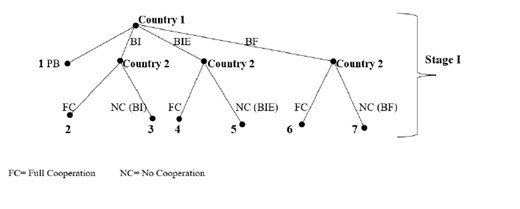
As mentioned in the text, country 1 starts to use BCA-threats if country 2 refuses the proposal 'cooperation' in stage 0 , which is our starting point as in Figure 1. That is, , and , as shown in Appendices A. 9 and B.3, and if according to Proposition 5.
If , cooperation (C) is established by the three BCAmeasures and we have three subgame-perfect Nash equilibria: , and , corresponding to endnodes 2,4 and 6 in the figure above. If , we have two subgame-perfect equilibria: and , corresponding to endnodes 4 and 6 in the figure above and finally for , the subgame-perfect equilibrium is with endnode 6 . For , the outcome is no cooperation (NC), with endnode 5 if because , whereas if , endnode 3 would emerge because in the Figure above. Thus, only for would we have a unique equilibrium, but not for . However, all other qualitative results would be the same as in Proposition 6.
Proof of Corollary 2
(i) As shown in Appendix A.9, the global welfare gap is given by , which increases in at an increasing rate. We showed in Proposition 6 that full cooperation cannot be achieved if , i.e., if is low or equivalently if is high, given .
(ii) Inserting the global welfare levels using Appendix A into Eq. (10) in the text, we obtain:
First, , where if and if . Th BI-regime is implemented if , where for all . Thus, we always have in the non-cooperative region.
Second, , where if and if . The BIE-regime is implemented if , and we have for all . Recall that the escalating penalty game starts from (see Assumption 1) and . Hence, in the non-cooperative region.
Third, , where 0 if and if . The BF regime could be implemented if , and we have for all . Hence, in the non-cooperative region.
References
Corresponding author
Output-based rebating is a variant of full BCAs. Rebates are provided for domestically produced output, regardless whether consumed domestically or exported (Fischer and Fox, 2012).
Some other papers focus on the legal issues of BCAs in relation to the regulation of the World Trade Organisation (WTO); see, for instance, Fischer and Fox (2012) and Mehling et al. (2019).
The way we model asymmetry allows us to distinguish between the level of damages, represented by the parameter, and the distribution of damages, represented by the parameter . An alternative formulation would be and with similar qualitative conclusions. The assumption of linear damages allows for the analytical tractability of the model.
The GATT allows WTO members to apply a border tax adjustment at a rate which is not higher than the rate applied to domestically produced "like" products.
That is, if could be chosen endogenously under the restriction . See for instance Hecht and Peters (2018).
Note that we cannot model BCAs on exports in the same way as on imports. That is, we cannot assume for instance because country 2 does not tax firm 1.
Thus, whenever the export rate is positive, the equilibrium tax on exports of firm 1 to country 2 is higher than the effective tax rate. Consequently, high equilibrium taxes do not necessarily imply high effective taxes.
Brander (1981) and Brander and Krugman (1983) suggest that the segmented markets model which provides a helpful setting for the analysis of strategic trade policy. Given constant marginal costs and a fixed number of firms, this setting allows separating the effects of trade policies and markets (in our model: import tariffs and export rebates). Import tariffs affect sales in country 1 , while export rebates affect the sales in country 2.
In Appendix A, we show that Nash equilibrium output levels always exist and are unique in each market. We also derive sufficient conditions for interior solutions.
Note that in Proposition 1, nothing is assumed about equilibrium taxes under all regimes and about the equilibrium value of under the BIE-regime. This is determined in stage 2. Hence, equilibrium or optimal emissions in Proposition 1 are generally viewed as a function of taxes, not only for equilibrium taxes.
The fact that equilibrium taxes (though not effective taxes) under the BIE- and BF -regime are equal is due to our assumption of a linear damage function.
Barrett (1994) proposed this term in an environmental agreement game without trade. In his context, either only small agreements are stable or if large agreements are stable, then the global gains from cooperation are small.

