


I investigate the interaction between a country that imports a commodity whose production contributes to a stock pollution from a country that produces that commodity. If the transboundary externality is priced improperly, the application of a tariff or border tax adjustment can provide an indirect policy instrument. But the imposition of such a tariff or tax creates an incentive for the producing country to deploy a domestic pollution tax. This, in turn, creates a strategic interaction between the two countries. Because the externality is linked to a stock pollutant, this strategic interaction will play out over time, which induces a dynamic game. In this modeling context, I describe the nature of the strategic interaction, and characterize the Markov-perfect equilibrium (MPE). Numerical results indicate that MPE can deliver long-run welfare levels similar to the social optimum program, and that the exporting country may be better off in the MPE than in the “business-as-usual” regime.
Introduction
International environmental problems featuring pollution spillovers such as climate change pose a special challenge since they have special features that distinguish them from national environmental problems. This point has specific implications for internationally traded products that are associated with greenhouse gas emissions. For example, imports of electricity into countries like England and Germany can come from Eastern Europe countries such as Poland. In these examples production of the exported commodity contributes to a flow of emissions, such as CO2, that accumulate in a stock that generates damages; moreover, there are likely to be differences between the valuation of these damages by the exporting and importing countries. In this context, feed-in tariffs or border tax adjustments can serve as a “second-best” instrument to limit the transnational pollution, playing a role for cross-border externalities that is somewhat similar to the role played by a Pigouvian tax.1 Similar considerations arise with trade in products that have embedded carbon emissions; this could apply to a host of products. Here too, one could imagine the importing country applying border tax adjustments on the basis of these embedded emissions, again as an indirect means of addressing the externality.
A handful of authors have explored to the potential use of trade instruments to control environmental externalities (Baumol and Oates, 1988; Markusen, 1975a,b; Parry and Oates, 2000); as a general rule, this extant literature has employed a static framework. But by its very nature the climate change problem is dynamic: environmental damages depend primarily on an accumulated stock, and they play out over a long time frame. There is also an existing literature that investigates the dynamic strategic incentives in transboundary pollution problems by using dynamic games. In these games, the players, usually the governments of countries, care about the stock of pollution, i.e., as pollution accumulates it affects the payoff to each country. Generally, the focus of these studies is a comparison between the cooperative scenario, which assumes a high degree of commitment to follow the agreed-upon pollution regulations, and non-cooperative scenario, in which each country’s environmental policy is selected to promote its own interest, given the other country’s emission standards (Barrett, 1994; Bayramoglu, 2006; Dockner et al., 2000; Dockner and van Long, 1993; List and Mason, 2001; Maler and de Zeeuw, 1998; Mason, 1997). This literature typically neglects the potential for a trade relationship among the countries involved in the transboundary pollution stock control. Notable exceptions include Fernandez (2002), who explores empirically dynamic solutions to transboundary pollution through trade liberalization and environmental institutions for multilateral pollution control, Cabo et al. (2001), who analyzed strategies that lead to a self-enforcing agreement on transboundary pollution problem within a North-South framework, Cabo et al. (2006), who study a model similar to ours, but with fixed output levels, Mason et al. (2015), who focus on the use of a feed-in tariff by the importing country, and Mason et al. (2018), who study the potential for the upstream country to lobby the downstream government to lower the import tariff. None of these papers explore the potential use of a climate-based strategy by the exporting country, such as a carbon tax, to blunt the effect of the importing country’s strategy. My goal in this paper is to evaluate such a strategic interaction.
I develop a dynamic model to investigate this problem. There are two countries, one of whom — country 1 — produces a commodity that contributes to a transboundary externality; this commodity is consumed in both countries. Because these damages become important over time, the relative weighting of future effects between the two countries is a potentially important concern. This distinction manifests itself in terms of divergent evaluations of the future damages associated with the stock pollutant; I adopt the limiting view of this asymmetry wherein the importing country — country 2 — bears damages but the exporting country does not.2 In this framework, country 2 applies a tariff (or a border tax adjustment) against imports from country 1 as an indirect measure to control the carbon externality. In response, country 1 applies a tax on consumption within its borders. The interaction thus described induces a differential game between the two countries. I assume that the strategic choices are indexed by the pollution stock, i.e., that the players use Markov strategies, and derive the Markovperfect equilibrium (MPE) to this differential game.3 I then provide numerical results to illustrate interesting features of the MPE. Three bear particular emphasis: 1) by introducing a consumption tax, country 1 induces country 2 to shift the time path of tariffs down; 2) for a range of parameter configurations, country 1 can be better off in the MPE than in the business-as-usual regime; 3) the MPE can deliver combined welfare levels that are a substantial fraction of those associated with the social optimum (first-best) regime.
Modeling Preliminaries
There are two countries, 1 and 2. I will sometimes refer to country 1 as the “upstream” country and country 2 as the “downstream” country. To facilitate development of analytic results, I focus on the discussion in this paper on a linear–quadratic specification.4 A single consumption good is produced in country 1 with a given fixed endowment of factors of production and a given technology. The associated cost of production is described by the function C(Q) = cQ2/2, where Q is the total amount produced. This output is sold to consumers in both countries, with Y referring to consumption in country 1 (i.e., the “home” country) and X referring to consumption in country 2 (i.e., the “away” country); Q = X + Y. Consumers within a particular country are homogeneous, but demand in country 1 differs from demand in country 2. I assume that demand in country k = 1, 2 is a downward-sloping, linear function of consumption in that country. To minimize notational clutter, I assume that demand in the two countries differs only via the intercept, i.e., the slope of inverse demands in the two countries are equal. Thus, quantity demanded in country k = 1, 2 is then Qk = (ak − pk)/b, where pk is the price paid by consumers in country k. I interpret aggregate utility in country k, Uk as consumer surplus:
Production in country 1 results in a flow of emissions. I assume that these emissions are proportional to output, and without loss of generality set units so that emissions equal output. These emissions contribute to the stock of pollution, Z, which evolves according to the following equation of motion:
where k represents the rate of pollution decay. The initial stock of the pollutant is Z0.
Although pollution is generated by emissions in country 1, for expositional clarity I assume that the environmental damages from the stock of pollution are only suffered in country 2.5 I also assume that there are no damages from the flow of emissions. Damages suffered in country 2 are d(Z) = δZ2/2.
Because these pollution externalities are exported from one country to another, no authority has the ability to intervene and enforce cooperation; countries will take actions to reduce emissions only if their efforts ultimately serve their own interest (Barrett, 1994; Sigman, 2002). While the downstream country cannot address the externality directly by imposing a Pigouvian tax on upstream producers, it can indirectly tackle the externality by imposing a tariff, τ, on imports X from country 1. The tariff lowers the upstream price, which induces firms to reduce their production — and with it the flow of emissions.
Because this reduction in output implies lower upstream net surplus, country 1 may be motivated to use some sort of pollution control instrument, so as to blunt the effect of the tariff; this indirect impact associated with country 2’s tariff is an important feature of my analysis. I assume that the instrument country 1 applies is a tax, σ, applied to domestic consumption.6
With a tariff in place, producers would receive p − τ in country 2, where p is the price paid by consumers in country 2. Firms would only be willing to sell in both countries if the price they receive in country 1 also equals p – τ. Accordingly, consumers in country 1 pay p – τ + σ. Producers are price-takers, and so their profit-maximizing production sets marginal cost equal to price: cQ = p–τ; thus, total output supplied in country 1 is:
Given any value of the tariff in country 2 and the consumption tax in country 1, the market-clearing conditions are Equation (2) and
Combining Equations (2)–4, and recalling that Q = X + Y, it is straight-forward to derive the equilibrium price received by sellers in terms of the upstream tariff and upstream tax:
where and is the equilibrium price in the absence of any taxes or tariffs.
Based on the tariff levied in country 2 and the tax in country 1, the quantity produced in country 1, the amount consumed in country 1 and the volume exported to country 2 are easily derived as
where is the amount produced in country 1, is the amount consumed in country 1, and is the amount exported to (and consumed in) country 2 in the absence of any taxes or tariffs. The comparative statics of tariff in country 2 and tax in country 1 follow immediately from Equations 5 to 8; I summarize these effects in the following Proposition.
Proposition 1. (a) An increase in the tariff levied in country 2 raises the equilibrium price and consumption in country 1, and lowers equilibrium production, emissions, and consumption in country 2; (b) an increase in the tax applied in country 1 lowers the equilibrium price, production, emissions, and consumption in country 1, and raises consumption in country 2.
Following the standard assumption of the “second-best” trade and environment literature, I assume that country 2 is able to influence the terms of trade through its tariff. To avoid any complications associated with the impact price effects might have upon consumption in country 2, I assume that any tariff revenues collected by country 2 are redistributed in a lump-sum fashion to downstream consumers. Likewise, any tax revenues collected by country 1 are redistributed in a lump-sum fashion to upstream consumers.
Net benefits for country 1 are given by the sum of consumer surplus and profit, the latter based on revenues from sales in each country; as I noted above, firms receive the price p – τ irrespective of sales venue, while consumers in country 1 pay p – τ + σ. Payoffs in country 1 can therefore be written as7:
Net benefits for country 2 are given by the sum of its consumer surplus and the tariff revenue, less the damages from the pollution stock, which can be written as8:
Because equilibrium exports and the upstream price are all function of the tariff and the consumption tax, net payoffs for each country are functions of τ and σ.
Baseline Solutions
Myopic (“Business-as-Usual”) Solution
I start by discussing a scenario where the downstream country, country 2, imposes a static tariff that is designed to maximize its flow payoff, and where the country 1 takes no action. In such a regime, upstream production generates a stream of emissions that obtain in the absence of any intervention intended to control the associated pollution stock. Such an environment is often referred to as “business-as-usual” in the climate economics literature; it is also myopic, in the sense that it ignores any dynamic effects.
Country 2’s flow payoffs are given in Equation 10; based on these payoffs, it is straightforward to show that country 2’s myopic tariff, , is9
Based on this tariff, output in country 1 is
In turn, this (constant) rate of output induces the time path of the pollution stock — as given by the exponential function
where is the steady-state stock in this regime. Armed with these expressions, it is straightforward to calculate the present discounted value of payoffs to each country, and in total, under the myopic regime.
Naive Solution
I next consider a regime where country 2 imposes a sequence of tariffs designed to address the evolving pollution stock, but where the upstream country does nothing in response. Because one might regard the lack of response by country 1 as indicative of a lack of sophistication, I refer to this regime as “naive.” As in the preceding sub-section, country 2’s flow payoffs are given by Equation 10. Country 2’s optimal tariff in this regime is time-varying, and is influenced by the shadow price θm, it places on the pollution stock; I show in the Appendix that this tariff satisfies:
where I use the definition from the preceding sub-section. Because the shadow value θm< 0, the following proposition follows immediately.
Proposition 2.Considering stock damages induces country 2 to levy larger tariffs.
Manipulating the condition above so as to replace the shadow value, one obtains a system of two linear, first-order differential equations — one for τ, and one for the pollution stock Z. The solution to this system is a pair of exponential functions
where ρ is a negative parameter given by Equation A.5, τ0 is a parameter given by Equation A.8, and the steady-state tariff and stock are
Armed with these expressions, it is straightforward to calculate the present discounted value of payoffs to each country, and in total, under the naive regime. I provide these calculations in Appendix A.1.
The Socially Optimal Solution
Before analyzing the equilibrium of the non-cooperative game between the two countries, I first discuss the socially optimal (cooperative) solution. To that end, suppose there is a global social planner whose goal is to choose the time paths of output and exports so as to maximize the discounted flow of the two countries’ combined payoffs. These combined payoffs equal the sum of the two countries’ utilities, less combined production costs, and less pollution damages. Thus, the cooperative problem can be cast as the choice of a time path of output that maximizes the discounted flow of aggregate benefits less production costs less pollution damages.
It is clear that this solution requires equating marginal utilities in the two countries; this ensures that maximal gross benefits are obtained. One may therefore define the aggregate benefit function
where consumption allocated to country 1 so that marginal utility is equated across the two countries10:
I show in Sub-section A.3 that the socially optimal time path of output takes the form
where ρ < 0 is given by Equation (A.28) and Q* is the steady-state level of production:
The associated time path of the pollution stock under the socially optimal program takes the form:
where Z* is the steady-state level of production:
Armed with these expressions, it is straightforward to calculate the present discounted value of payoffs to each country, and in total, under the socially optimal regime. I provide these calculations in Appendix A.3.
The Non-cooperative Equilibrium
I now turn to an analysis of the non-cooperative equilibrium of the strategic interaction between the two countries. Because each country’s policy instrument is likely to depend on the level of the pollution stock, the natural focus is on Markov strategies. The solution concept I apply is Markov-perfect equilibrium (MPE), which requires each player’s action to be optimal given the other player’s strategy, for every stock level; as such, the strategy combination is subgame-perfect. Because the structure of the game is linear–quadratic, it is also natural to focus attention on linear Markov strategies. If there is an MPE in linear strategies, the two countries’ policies can be described by
Determination of the MPE then boils down to identifying the four parameters τ0, τ1, σ0, and σ1.
Before proceeding to a discussion of the MPE, I discuss the implications of the system embodied in Equations 20–21. Inverting Equation 21 allows one to express the pollution stock in terms of country 1’s Markov strategy:
inserting into Equation 20 then produces
Equation 22 highlights a key point in my analysis, summarized in the following proposition:
Country 2 regards the two policies as strategic substitutes when the slope coefficients in the two countries Markov strategies are of opposite sign.
This strategic substitutability arises naturally from the nature of equilibrium output, Equation 6, which shows output is driven by the sum of the downstream tariff and the upstream tax. This fact, together with the fact that the trajectory of the pollution stock is directly influenced by output, underpins country 1’s ability to induce country 2 to lower its tariff trajectory by shifting up the path of consumption taxes. In particular, introducing a consumption tax will lower the trajectory of tariffs (a feature of the simulations discussed below).
I now describe the two countries’ optimization problems, starting with country 2.
Country 2’s Optimization Problem
The optimization problem for country 2 is to choose the time path of the tariff so as to maximize the discounted flow of its net benefit function over time, given the strategy that 1 employs. Letting σ(Z) denote 1’s Markov strategy and r the discount rate, and taking note of Equation 10, 2’s optimization problem is:
I show in the Appendix that country 2’s optimal tariff can be described by
With a positive consumption tax in country 1, and since the shadow cost of the pollution stock is negative, it follows that country 2’s Markov tariff is larger than the myopic tariff; as I noted above the Markov tariff lies below the naive tariff. These points are summarized in the following proposition.
Proposition 4.Country 2’s Markov tariff lies between the myopic and naive tariffs.
The solution to country 2’s problem also entails a characterization of the time path of the shadow value (cost) of the pollution stock; this is given by11
Country 1’s Optimization Problem
The optimization problem for country 1 is to choose the time path of the consumption tax so as to maximize the discounted flow of its net benefit function over time, given the strategy that country 2 employs. Letting τ(Z) denote 2’s Markov strategy, and taking note of Equation 9, country 1’s optimization problem is:
where, from Equation 7,
I show in the Appendix that country 1’s optimal tax is:
The solution to country 1’s problem also entails a characterization of the time path of the shadow value (cost) of the pollution stock; this is given by
The MPE is determined by the solution to a pair of first-order linear differential equations, one for τ and one for σ; existence of a solution over some compact set of stocks follows from standard theorems (see, e.g., Boyce and DiPrima (2005, pp. 68–70)). I summarize this observation in the following Proposition.12
Proposition 5.There is a Markov-perfect equilibrium consisting of linear strategies in terms of the pollution stock: τ(Z) = τ0+τ1Z, σ(Z) = σ0+ σ1Z.
Armed with these expressions, it is straightforward to calculate the present discounted value of payoffs to each country, and in total, in the MPE. I provide these calculations in Appendix A.2.
Numerical Illustration
To flesh out the model, I evaluate a particular parameterization. The parameters chosen for this numerical illustration are largely chosen for computational convenience; later, I consider the effect of varying certain parameters. I set the demand parameters so that there is larger demand in country 2 than country 1, which seems consistent with the idea that country 1 exports to country 2; the parameters used are a1 = 160, a2 = 200, b = 1. I also set the marginal cost parameter c = 1. The discount rate is taken to be r = .05, which also equals k, the depreciation rate for the pollution stock. Finally, I set δ, the parameter in the damage function, equal to .01.
Using these parameters, in conjunction with Equations A.18– A.21 in the Appendix, one can calculate the parameters in the two country’s Markov strategies. The resultant strategies are:
I note that the slope coefficients are of opposite sign; from proposition 3 it then follows that country 2 views the two policies as strategic complements.
The parameter values in the two Markov strategies are linked to the underlying exogenous parameters, particularly the demand coefficient (b), the marginal cost coefficient (c), and the decay rate in the pollution stock (k). To get a feel for how these three parameters influence the countries’ Markov strategies, I re-ran the numerical algorithm allowing for three possible values for each of the three parameters; there are therefore 3 x 3 x 3 = 27 combinations of the three parameters. For both b and c I consider values 10% smaller and 10% larger than the value used in the baseline analysis; for k I use values 20% smaller and larger than the baseline value. I denote the larger potential values with the label “H” (for ‘high’) I denote the smaller potential values with the label “L” (for ‘low’); the baseline value is referred to with the label “M” (for ‘medium’). The combinations are thus denoted as triples “LLL” . . . “HHH”. In this notation, the first letter refers to the value for b, the second letter refers to the value for c, and the third letter refers to the value taken by k. Table 1 summarizes the relevant information. In this table, the combination is listed in the first column, with the corresponding values for the three parameters b, c, and k listed in columns 2–4. Columns 5 and 6 list the intercept coefficients for country 1 and country 2’s Markov strategies, while columns 7 and 8 list the slope coefficients. Key features of this exercise are summarized in the following statement.13
Numerical Result 1: For the range of parameters considered in Table 1: a) τ1 is always positive and σ1 is always negative; b) τ0 is increasing in each of b, c, and k; c) σ0 is increasing in b and decreasing in c and k, c) τ1 is increasing in b and decreasing in c and k, and d) σ1 is decreasing in b and c and increasing in k.
After determining the coefficients in the Markov strategies, one can determine the trajectory of the pollution stock by employing Equation 6 to write Q in terms of Z, and then using that expression in conjunction with Equation (1). Once Z has been derived, inserting that back into Equations 20 and 21 determines τ and σ. I plot the resultant trajectories, based on the Markov strategies for the parameter configuration MMM, in Figure 1. Panel (A) of this figure shows the trajectories of the downstream tariff and upstream tax, while panel (B) shows the trajectory of the pollution stock. For comparison purposes, I overlay the trajectory of the tariff under the naive regime in panel (A), and the corresponding pollution stock in panel (B). This diagram illustrates one of the main themes of the paper: by introducing a consumption tax, country 1 induces country 2 to lower its tariff; panel (A) suggests that for this parameterization, the effect is quite marked. In the absence of a consumption tax, country 2’s tariff rises sharply, with the pollution stock rising only slightly. But when a consumption tax is levied, country 2’s tariff rises quite slowly; the combined effect of the consumption tax and tariff upon output produced in the upstream country is less than the original (naive) tariff, and so the pollution stock grows more in the MPE than in the naive regime.
MPE strategy coefficient values.
| comb’n | b | c | k | τ0 | σ0 | τ1a | σ1b |
|---|---|---|---|---|---|---|---|
| LLL | 0.9 | 0.9 | 0.04 | 15.12 | 55.61 | 0.886 | –0.95 |
| LLM | 0.9 | 0.9 | 0.05 | 15.89 | 53.8 | 0.742 | –0.933 |
| LLH | 0.9 | 0.9 | 0.06 | 16.62 | 52.38 | 0.635 | –0:917 |
| LML | 0.9 | 1 | 0.04 | 15.37 | 54.17 | 0.807 | –0.956 |
| LMM | 0.9 | 1 | 0.05 | 16.15 | 52.45 | 0.673 | –0.936 |
| LMH | 0.9 | 1 | 0.06 | 16.87 | 50.98 | 0.56 | –0.908 |
| LHL | 0.9 | 1.1 | 0.04 | 15.59 | 52.7 | 0.735 | –0.957 |
| LHM | 0.9 | 1.1 | 0.05 | 16.37 | 50.96 | 0.599 | –0.925 |
| LHH | 0.9 | 1.1 | 0.06 | 17.08 | 49.52 | 0.491 | –0.889 |
| MLL | 1 | 0.9 | 0.04 | 15.81 | 56.75 | 1.019 | –1.021 |
| MLM | 1 | 0.9 | 0.05 | 16.59 | 54.93 | 0.862 | –1.007 |
| MLH | 1 | 0.9 | 0.06 | 17.3 | 53.35 | 0.726 | –0.985 |
| MML | 1 | 1 | 0.04 | 16.08 | 55.56 | 0.936 | –1.034 |
| MMM | 1 | 1 | 0.05 | 16.87 | 53.78 | 0.785 | –1.014 |
| MMH | 1 | 1 | 0.06 | 17.58 | 52.26 | 0.658 | –0.987 |
| MHL | 1 | 1.1 | 0.04 | 16.32 | 54.26 | 0.859 | –1.038 |
| MHM | 1 | 1.1 | 0.05 | 17.09 | 52.46 | 0.705 | –1.008 |
| MHH | 1 | 1.1 | 0.06 | 17.81 | 50.96 | 0.582 | –0.973 |
| HLL | 1.1 | 0.9 | 0.04 | 16.43 | 57.55 | 1.154 | –1.086 |
| HLM | 1.1 | 0.9 | 0.05 | 17.21 | 55.73 | 0.98 | –1.075 |
| HLH | 1.1 | 0.9 | 0.06 | 17.92 | 54.15 | 0.836 | –1.057 |
| HML | 1.1 | 1 | 0.04 | 16.72 | 56.63 | 1.068 | –1.106 |
| HMM | 1.1 | 1 | 0.05 | 17.49 | 54.74 | 0.893 | –1.084 |
| HMH | 1.1 | 1 | 0.06 | 18.22 | 53.25 | 0.759 | –1.063 |
| HHL | 1.1 | 1.1 | 0.04 | 16.96 | 55.45 | 0.978 | –1.112 |
| HHM | 1.1 | 1.1 | 0.05 | 17.74 | 53.66 | 0.815 | –1.086 |
| HHH | 1.1 | 1.1 | 0.06 | 18.46 | 52.12 | 0.677 | –1.052 |
Note:
Scaled by 10–3.
Scaled by 10–2.
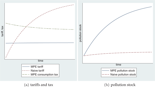
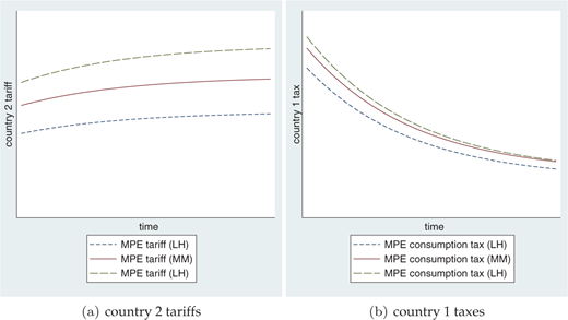
Figure 2 explores the sensitivity of the Markov strategies to the ratio of inverse demand slope to marginal cost slope, b/c.14 Here I plot three trajectories for both the Markov tariff and the Markov tax, based on three parameter combinations. These combinations are LH (low b, high c), the combination MM that underlies Figure 1 (medium b, medium c), and HL (high b, low c). The apparent effect of raising the ratio b/c is to shift up the Markov tariff and shift down the consumption tax, though none of these effects is large: the effect corresponds to an elasticity of about 1.5 for the slope of the Markov tariff and less than one for intercept of the tariff, and both slope and intercept of the tax.15
The next question to be investigated regards the level of well-being under the MPE, as compared with the other regimes. Figure 3 gets at this issue from the social perspective. Here, I plot the ratio of present discounted value under the MPE to the socially optimal regime, across various levels of the underlying exogenous parameters. Panel (A) shows this relation for the pollution decay rate (k), panel (B) for the interest rate (r), panel (C) for the inverse demand slope (b), and panel (D) for the marginal cost slope (c). The key message here is that the MPE delivers a combined level of well-being that is at or above 70% of the social optimum. For small levels of the pollution decay rate, the ratio is even larger — approaching 100% as k becomes small. This observation takes on special significance for problems in which the pollutant is very long-lived, as with atmospheric carbon. At the other extreme, the presented discounted value associated with the MPE falls off when pollution decays rapidly. The intuition is that when pollution is long-lived, sophisticated strategies that are particularly mindful of dynamic effects, such as the MPE, are particularly beneficial; these benefits become much less important when pollution decays rapidly, so that dynamic effects are less pronounced.
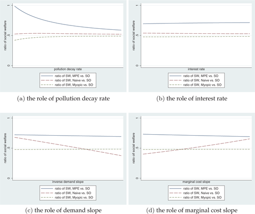
Relative increase in social welfare, various regimes.
Relative increase in social welfare, various regimes.
A related question has to do with the potential gain associated with migrating from the “Business-as-usual” (BAU, or myopic) regime. To get at this idea, I computed the ratio of the increase in combined present discounted value from the MPE less the BAU present discounted value, as compared to the gain in present discounted value from the socially optimal program less the present discounted value under the BAU regime. I refer to this construct as the “percentage of increased welfare captured in MPE”, and plot it against each of the four exogenous parameters in Figure 4. The evidence from this series of graphs corroborates the messages from Figure 3: the MPE captures a substantial share of the potential gain reflected by the difference between present discounted values under the socially optimal program versus the BAU regime. For b, c, and r this share of potential gains is relatively constant and near, but a bit less than, 50%. For the pollution decay rate, k, the share of potential gain is large — approaching 100% — when the decay rate is small (though it falls of as k is increased). Again, this point carries particular importance for problems like climate change. I summarize the results from Figures 3 and 4 in the following.
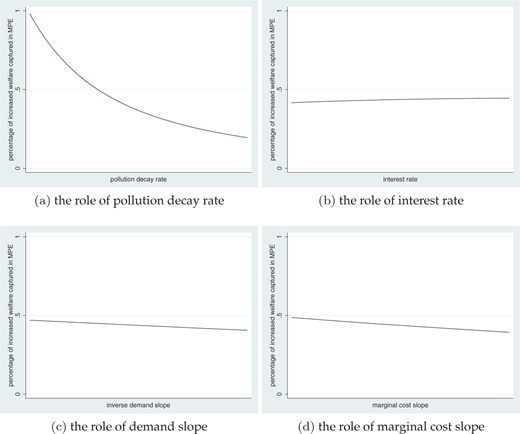
Relative increase in global welfare from Markov-perfect equilibrium.
Relative increase in global welfare from Markov-perfect equilibrium.
Numerical Result 2: In the numerical simulations reported in this paper, the Markov-perfect equilibrium: a) delivers a significant share of the socially optimal present discounted value; and b) captures roughly half the potential gains in social welfare associated with moving from business-as-usual to the first-best regime.
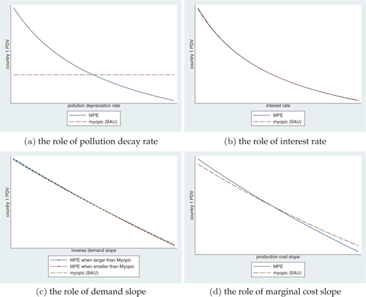
The final issue I investigate relates to a comparison of the present discounted value of payoffs to country 1 under the MPE as compared to the BAU regime. One might naturally suspect that adopting some form of quantity limiting instrument, such as a tariff or a tax, would reduce the upstream country’s well-being. But a surprising result in my model is that the upstream country can, under some circumstances, be better off in the MPE than in the BAU regime. The intuition is that imposing a consumption tax generates two effects which could be beneficial to country 1: first, it captures some of the wealth that would otherwise be transferred to country 2; second, as I noted above by by adopting a consumption tax country 1 influences country 2 to lower its tariff. These effects run against the natural intuition, leaving the net effect in question. Figure 5 addresses this issue. Here, I plot the PDV for country 1 under the two regimes of interest: the MPE (which I plot as a solid line, with the exception of the comparison related to b, as discussed below) and the myopic BAU regime (plotted as a dashed line). I graph these values against the four exogenous parameters identified above: Panel (A) shows this relation for the pollution decay rate (k), panel (B) for the interest rate (r), panel (C) for the inverse demand slope (b), and panel (D) for the marginal cost slope (c). For two of these comparisons, the difference between the two PDVs does not change much as the exogenous parameter is varied — this obtains for the interest rate, r, and the inverse demand slope, b.
Relative increase in global welfare from Markov-perfect equilibrium.
Relative increase in global welfare from Markov-perfect equilibrium.
As panel (B) shows, the PDVs are very similar at every value of r. This is a reflection of the fact that the PDVs are quite similar in the baseline case discussed above, and that the difference between the two PDVs is insensitive to the interest rate. For the inverse demand slope, there is a noticeable effect, though the scale of panel (C) makes it somewhat hard to pick out this effect. To help the reader identify the pattern, I plot the level of PDV under the MPE using diamonds for those values of b where country 1 is better off in the MPE, and with circles for those values of b where country 1 is better off under the BAU regime. While the differences in PDVs are not large, it is apparent that the upstream country fares better under the MPE when demand is relatively inelastic (i.e., b is smaller). Panel (A) shows that country 1 fares better when the pollution decay rate k is smaller than when it is larger; this echoes points regarding the comparative dynamics related to k I discussed above. Finally, panel (A) shows that country 1 fares better when the marginal cost slope c is smaller than when it is larger. I summarize the key takeaway message from this set of simulations in the following.
Numerical Result 3: For a range of the parameter configurations reported in this paper, country 1 is better off in the Markov-perfect equilibrium than in the business-as-usual regime.
Concluding Remarks
Concerns about limiting carbon emissions have recently led some OECD countries to invoke feed-in tariffs and border tax adjustments. These instruments serve two purposes: they increase the cost of associated products in the importing country, reducing the level of consumption; they also increase the cost of doing business in the importing country, inducing the exporting country to adjust its behavior. Under an optimistic view of these incentives, the exporting country will limit emissions, and perhaps invoke some sort of climate policy; the potential for such adaptation is most intriguing for transitioning countries such as those found in Eastern Europe.
In this paper I showed existence of Markov-perfect equilibrium (MPE) in a game between two countries, a country (which I call “country 1”) whose production generates a flow pollutant, such as carbon dioxide, and a country (which I call “country 2”) that suffers harm from the stock of that pollutant. Country 1’s production trades internationally, and so country 2 has an indirect method to influence country 1’s emissions: by imposing a tariff, country 2 effectively taxes the source of pollution. In light of this structure, the country 1 is motivated to impose a tax its product — even if country 1 suffers little or no harm — as this will induce country 2 to lower its tariff. In this setting, the combination of importing country tariff and producing country tax serves to reduce the flow of emissions below the level that would otherwise be observed. Even so, the resultant flow of emissions exceeds the socially optimal level. Numerical analysis of this problem indicates that the MPE delivers between 40% and 50% of the potential welfare gains associated with moving away from the myopic “business-as-usual” regime; the gains associated with the MPE can approach 100% of potential gains for very slowly decaying pollutants.
The essential feature of this set of results is that the importing country is able to induce lower emissions through two channels: there is a direct effect, as the imposition of a tariff is akin to an emissions tax. But there is also an indirect effect: by creating a financial environment wherein the country 1 has an incentive to curtail production (so as to lower emissions), country 2 motivates country 2 to tax its own product. This effect arises because the two instruments are strategic substitutes. Accordingly, a policy environment that allows the country suffering harm from the stock pollutant to tax the associated (imported) production can be doubly beneficial.
Appendix A. Derivations in the Linear-Quadratic Model
In this Appendix I provide mathematical details for the derivation of the Naiive, Markov-perfect and Socially optimal equilibria.
A.1 Naive Regime
In this regime, country 2 imposes a sequence of tariffs designed to maximize the present-discounted flow of its welfare; as in the myopic regime, country 1 does not impose a tax regime. The naive regime differs from “business-as-usual” in that country 2 imposes a time-varying tariff, based on the impact of stock damages. As such, country 2’s flow payoff is given by Equation 10; the dynamic optimization problem it solves is
The current-value Hamiltonian for this optimization problem is
where θn is 2’s shadow value of pollution in the naiive regime and I have used the fact that in this regime. Pontryagin’s maximum principle gives the necessary conditions for the solution to this dynamic optimization problem; in light of Equation 4, these conditions can be written as:
as well as the transversality condition . Straight-forward algebraic manipulation of Equation A.1 yields:
It then follows that
This equation, together with Equation (1), yields a system of two first-order, linear differential equations that govern the time paths of tariff and pollution stick in the myopic regime. This system can be expressed in matrix form as
The solution to this system is given by the combination of a general solution to the homogeneous system (obtained by setting the right-hand side to the zero vector) and a specific solution to the full system.
Because the system consists of linear first-order differential equations, the general solution is based on the exponential function eρt, with
and ; the pair represents the steady-state combination of tariff and pollution stock.
Using those functions, the homogeneous equation is:
This equation must hold for all values of τ and Z, which implies, that the matrix on the left-hand side must be singular, and hence its determinant must be zero. This observation leads to the characteristic equation:
There are two roots to this equation, one positive and one negative; i.e., the system is saddle-point stable. Stability of the system then requires that the solution is based on the negative root
The solution in the naïve regime then is described by:
where
are the steady-state pollution stock and tariff in the naÃŕve regime.
The solution is completed by determining the coefficients τ0 and Z0.
The initial condition Z(0) = Z0 determines the latter, since at t = 0; thus, . Next, I observe that Equation A.6 implies ˙τ = ~
ρτ0 at t = 0, while Equation A.4 implies
again, at t = 0. It follows that
A.2 Non-cooperative Solution
I now turn to the analysis of the Markov-perfect equilibrium (MPE) in the Linear–Quadratic Model. The solution is built up from the optimization decisions for the two players, which I obtain by applying Pontryagin’s maximum principle. Before conducting that analysis, I first observe that Equations 6–8 imply and ; also, taking note of Equations 20–21, Equation (1) can be expressed as
I start with player 2. Letting σ(Z) denote player 1’s Markov strategy, player 2’s optimization conditions are based on the current-value Hamiltonian
as well as the transversality condition Straight forward manipulation of Equation A.10 yields Equation 23, while Equation A.11 corresponds to Equation 24.
Next, consider player 1. Letting σ(Z) denote player 2’s Markov strategy, player 1’s optimization conditions are based on the current-value Hamiltonian
and defining , the optimization conditions are
as well as the transversality condition Straight-forward manipulation of A.12 yields 23, while A.13 corresponds to 26.
Next, I proceed by time-differentiating Equations A.10 and A.12, and then using the system A.10–A.13 to substitute for
This yields:
These equations must match the equations of motion for the shadow values, Equations A.11 and A.13. These latter equations can be distilled by using Equation 8 to substitute for X and Equations 23 and 25 to substitute for θ and ξ; doing so yields:
For Equations A.14 and A.16 to match for all values of Z, the intercepts in the two equations must be equal, and the slope coefficients in the two equations must be equal. Likewise, For Equations (A.15) and A.17 to match for all values of Z, the intercepts in the two equations must be equal, and the slope coefficients in the two equations must be equal. This gives rise to four equations:
The four parameters in the linear Markov strategies are given by the solution to the system of four Equations A.18–A.21. I note that Equations A.19 and A.21 do not contain τ0or σ0, and so these two equations can be used to solve for τ1 and σ1. Using the resultant values, one can then use Equations A.18 and A.20 to solve for τ0 and σ0.
A.3 Socially Optimal Solution
Finally, I analyze the socially optimal (cooperative) solution. Here, the goal is to determine the time paths of the level of total production and the distribution of that production between the two markets that maximize the combined present discounted payoffs. Denote the discounted net benefits for country j = 1, 2 by these are:
Let . The distribution of output Q between the two countries equates marginal benefits, which requires , so that
It follows that
where m is the (cooperative) shadow value of the pollution stock, which, as pollution is a bad, one presumes is negative. The optimality rule for the cooperative solution is then
The solution also requires the evolution of the shadow value satisfy
where r is the (common) discount rate.
The evolution of the socially optimal quantity may be derived by time-differentiating Equation (A.24), which yields
Combined with Equation (1), this yields the system of first-order, linear differential equations:
The solution to this system is given by the combination of a general solution to the homogeneous system (obtained by setting the right-hand side to the zero vector) and a specific solution to the full system. Because the system consists of linear first-order differential equations, the general solution is based on the exponential function eρt, with Q = ωeρt and . Using those functions, the homogeneous equation can be expressed as:
Because this equation must hold for all values of Q and Z, the matrix on the left-hand side must be singular; this implies that the determinant is zero, which leads to the characteristic equation:
As Q is convex and negative at ρ = 0, it follows that the two roots are ρa < 0 < ρb; i.e., the system is saddle-point stable. Of these, we select the negative root to ensure stability:
The specific solution is given by the steady-state cooperative values Q*, Z*:
The complete solution is then
Since Z = Z0 at time t = 0, it follows that
Moreover, time-differentiating Equation (A.30) yields
where I have used the fact that Q* = kZ* by definition of the steady state. Comparing these two expressions for , I obtain:
Putting everything together, I obtain
A.4 Equilibrium Payoffs
I conclude by deriving the present discounted value of payoffs realized by each of the countries, under both the Markov-perfect and socially optimal (cooperative) equilibria.
Markov-perfect
I start by adopting some useful terminology:
Using this notation, Equation A.9 can be written as:
It is easy to see that the solution to this differential equation is
Moreover, with η3 > 0 the limiting value of Z is , which is the steady-state value of Z. The initial condition on Z then determines η0 as
The key ingredients in describing the countries’ flow payoffs are Q, output produced in country 1, and X, exports from country 1 to country 2. Using the notation above, these are:
The flow payoffs in country 1 can then be written as:
where
Likewise, the flow payoffs in country 2 can be written as:
where
The PDVs of welfare flows for the two countries are based on the integrals of Z and Z2:
Combining these ingredients, we have
Socially Optimal
Recalling that in the cooperative regime, the flow payoffs to each country can be written as
Then recalling the expressions for output and pollution stock along the equilibrium path, given in Equations (A.31)–(A.32), and recalling ωa= Z0 – Z*, the present-discounted flow of payoffs to country 1 can be written as
Similarly, the present-discounted flow of payoffs to country 2 can be written as
See Copeland (1994, 1996) andSnape (1992). It is not clear whether border tax adjustments in energy markets are compatible with World Trade Organization laws governing international trade; feed-in tariffs might be justified by the World Trade Organization regulations (Article XX which allows for exceptions to general GATT principles) since production of the traded good is a direct cause of environmental damages occurring in the importing country. Biermann and Brohm (2005) provide a detailed discussion of the potential legal ramifications. For a model of dynamic interactions among countries that value environmental damages identically, seeYanase (2010).
Alternatively, one could envision a situation where the exporting country places little weight on future effects, while the importing country cares very much about the future. Adopting a similar simplification, List and Mason (2001) investigate the potential for differing national policies to produce preferable outcomes to a common pollution control measure.
My analysis is similar in spirit to Liski and Tahvonen (2004), although they ask a different question. In their paper, the interaction is between a coalition of oil producing buyers, such as the EU, and a coalition of sellers, such as OPEC. The buyers institute a time path of taxes on oil, which induces the sellers to adjust their time path of oil prices; a major focus of their analysis is the distribution of rents associated with oil trade. By contrast, my focus is on the ability of strategic interactions to generate socially attractive reduction in carbon emissions.
For an analysis in a more general framework, seeMason (2017).
List and Mason (2001) take a similar approach. As they note, one can think of this scenario as characterizing a situation where one country bears the brunt of the damages; allowing for damages in both countries greatly complicates the analysis without changing the qualitative results. An alternative approach would be to assume the government in country 1 does not care about the damages borne by its citizenry.
One might think that it would be more natural for country 1 to impose a tax on production. But as noted by Mason et al. (2015), such a policy can be preempted by country 2, in the sense that the tariff that is optimal for country 2 will generally drive the upstream tax to zero. In light of this result, country 1 needs to find an alternative instrument; since taxing local consumption can influence something that country 2 cannot impact, using such a policy can generate net gains for country 1.
Net welfare in country 1 is , where , and Q = X + Y. From Equation (2), p – τ = cQ. Combining terms then yields the expression in the text.
Net welfare in country 2 is W2= U2(X) + τX – d(Z), where U2(X) = a1Y – bY2/2. From Equation 4, p = a2–bX. Combining terms then yields the expression in the text.
This tariff solves . Using Equation 8 (with σ = 0), one has accordingly, . The expression in the text then follows directly.
Equating marginal utilities: a1 – bY = a2 – bX, so that a1 – a2 = b(Y – X) = b(Q – 2X).
Note that θ must be negative. If it were positive, it would grow at least as fast as e(r+kt). As a result, θ(t)Z(t)e–rt would grow at least as fast as Z(t)ekt, which grows without bound as t goes to ∞. It follows that the shadow value is negative, and that it tends to be a long-run equilibrium level.
It has been pointed out that there are also (many) equilibria in non-linear strategies (Dockner and van Long, 1993; Tsutsui and Mino, 1990). I focus on linear strategies here for expositional simplicity, and because I believe that a strong case can be made that linear strategies are focal.
A simple ordinary least squares regression identifies the first-order effects of changing one of the exogenous parameters in isolation, which underpin the comparative dynamics articulated in the Numerical Result. I note also that the largest absolute impact comes from k, and this impact is an order of magnitude larger for τ0, σ0, and τ1 (and three times as large as the other effects for σ1).
This ratio, which is directly related to , plays an indirect role in many of the characterizations in the analysis.
Starting from the combination MMM, the movement to the short-dashed line in Figure 2 represents a reduction of b/c from 1 to .818, or about 18%; referring back to Table 1, the resultant change in the intercept of country 2’s tariff is about a 3% reduction (from 16.87 to 16.37), while the impact on its slope is about a 24% reduction (from .785 to .599). The elasticity of the intercept is thus around 1/6, while the elasticity of the slope is about 1.5. For country 1, the effects are similar or smaller: the intercept of its Markov tax falls by about 5% (from 53.78 to 50.96), while its intercept rises about 9% (from –1.014 to –.925); accordingly, the elasticity of both intercept and slope for the upstream tax are both less than one in magnitude.
The optimal tariff is also subject to the constraint that τ is no smaller than the tariff that maximizes country 2’s static net surplus; in practice, this constraint never binds.
The optimal tariff is also subject to the constraint that τ is no smaller than the tariff that maximizes country 2’s static net surplus; in practice, this constraint never binds.

