


In this paper we study a class of complexity measures, induced by a new data structure for representing k-valued functions (operations), called minor decision diagram. When assigning values to some variables in a function the resulting functions are called subfunctions, and when identifying some variables the resulting functions are called minors. The sets of essential variables in subfunctions of are called separable in .
We examine the maximal separable subsets of variables and their conjugates, introduced in the paper, proving that each such set has at least one conjugate. The essential arity gap of the function is the minimal number of essential variables in which become fictive when identifying distinct essential variables in . We also investigate separable sets of variables in functions with non-trivial arity gap. This allows us to solve several important algebraic, computational and combinatorial problems about the finite-valued functions.
1. Introduction
The complexity of finite operations is still one of the fundamental tasks in the theory of computation and besides classical methods like substitution or degree arguments a bunch of combinatorial, and algebraic techniques have been introduced to tackle this extremely difficult problem.
A logic gate is a physical device that realizes a Boolean function. A logic circuit is a direct acyclic graph in which all vertices except input vertices carry the labels of gates. When realizing n-variable k-valued functions the circuit is called the -circuit or Multi-Valued Logic circuit (MVL-circuit).
To move from logical circuits to MVL-circuits, researchers attempt to adapt CMOS (complementary metal oxide semiconductor), I2L (integrated injection logic) and ECL (emitter-coupled logic) technologies to implement the many-valued and fuzzy logics gates. The MVL-circuits offer more potential opportunities for the improvement of present VLSI circuit designs. For instance, MVL-circuits are well-applied in memory technology as flash memory, dynamic RAM, and in algebraic circuits [4].
In this paper we investigate a method for reduction of finite valued functions, namely by their identification minors. This method is a basic model of computing with MVL-circuits corresponding to collapsing of some inputs in the circuits. We, also study the computational complexity of this method and classify the functions in finite algebras for small values of k and n under such complexity.
Computational complexity is examined in concrete and abstract terms. The concrete analysis is based on models that capture the exchange of space for time. It is also performed via the knowledge about circuit complexity of functions. The abstract analysis is done via complexity classes, the classification of data structures, functions etc. by the time and/or space they need.
There are two key methods for reduction (computing) of the k-valued functions which are realized by assigning constants or variables to their inputs. Then the resulting objects are: subfunctions or minors, respectively. These reductions are also naturally suited to complexity measures, which illustrate “difficulty” of computing as the number of subfunctions, separable sets, and minors of the functions.
Another topic in complexity theory is to classify finite functions by their complexity such that the functions are grouped into equivalence classes with same evaluations of the corresponding complexities. Each equivalence relation in the algebra of k-valued functions determines a transformation group whose orbits are the equivalence classes (see [8,10,12]. Using the lattice of Restricted Affine Groups (RAG) in [15] we have obtained upper bounds of different combinatorial parameters of several natural equivalences in for small values of k and n. In the present paper we follow this line to study assigning (not necessarily unique) variable names to some of the input variables in a function f. This method of computing consists of equalizing the values of several inputs of f.
Section 2 introduces the basic definitions and notation of separable sets, subfunctions, minors, arity gap, etc. An important result, namely if a function has non-trivial arity gap then all its sets of essential variables are separable, complements this section. Section 3 examines the ordered decision diagrams (ODD), minor decomposition trees (MDTs) and minor decision diagrams (MDDs) of k-valued functions. In Section 3.3 we treat the minor complexities of functions with their classifications by the transformation groups. Section 4 is an illustration of the results in the paper applied to the simplest case of Boolean functions. In the Appendix we provide a classification of all ternary Boolean functions with respect to the minor complexity.
2. Subfunctions and minors of functions
A discrete function f is defined as a mapping: where the domain and the range B are non-empty finite or countable sets. Let be a countable set of variables and let denote the set of the first n variables in X. Let k be a natural number with . Let denote the set . The operations addition “” and product “.” modulo k constitute as a ring. An n-ary k-valued function (operation) on is a mapping for some natural number n, called the arity of f. denotes the set of all n-ary k-valued functions and is called the algebra of k-valued logic. It is well-known fact that there are functions in . For simplicity, let us assume that throughout the paper we shall consider k-valued functions, only.
For a given variable x and is defined as follows:
The ring-sum expansion (RSE) of a function f is the sum modulo k of a constant and products of variables or , (for ) of f. For example, is a RSE of the function f in the algebra , with and , otherwise. Any k instances of the same product in the RSE can be eliminated since they sum to 0. Throughout the present paper, we shall use RSE-representation of functions.
Let and let be the set of all variables, which occur in f. We say that the i-th variable is essential in f, or f essentially depends on , if there exist values , such that
The set of all essential variables in the function f is denoted and . The variables from which are not essential in are called inessential or fictive.
Let be an essential variable in f and let c be a constant from . The function obtained from by assigning the constant c to the variable is called a simple subfunction of f (sometimes termed a cofactor or a restriction). When g is a simple subfunction of f we write . The transitive closure of is denoted . is the set of all subfunctions of f and .
Let and let with , , and for . Then we write or equivalently, . For brevity, sometimes we shall also use the notation or .
We say that each subfunction g of f is a reduction to f via the subfunction relationship.
A non-empty set M of essential variables in the function f is called separable in f if there exists a subfunction g, such that . denotes the set of all the separable sets in f and .
The theory of separable sets (TSS) has been developed in the work of many mathematicians since the middle of the last century – K. Chimev [2], A. Salomaa [11], J. Denev, I. Gyudzhenov [7], Sl. Shtrakov [3] etc. TSS is important to avoid any redundancies when computing discrete functions and other structures as graphs [2], terms [14], etc.
Let and be two distinct essential variables in f. The function h is obtained from by identifying (collapsing) the variables and , if
for all .
Briefly, when h is obtained from f, by identifying the variable with , we write and h is called a simple identification minor of f. Clearly, , because , but it has to be essential in f. When h is a simple identification minor of f we write . The transitive closure of is denoted . is the set of all distinct minors of f and . Let be an identification minor of f. The natural number is called the order of the minor h of f.
We say that each minor h of f is a reduction to f via the minor relationship.
Let denote the set and let , for all .
Let be an n-ary k-valued function. The essential arity gap (shortly arity gap or gap) of f is defined as follows
Let . We let denote the set of all k-valued functions which essentially depend on m variables whose arity gap is equal to p, i.e.
We say that the arity gap of f is non-trivial if . It is natural to expect that the functions with “huge” gap, have to be more simple for realization by MVL-circuits and functional schemas when computing by identifying variables.
An upper bound of for Boolean functions is found in K. Chimev [2] and A. Salomaa [11], showing that . In [18] R. Willard also proved that if a function depends on n variables and , where then . It is clear that . Thus in all cases .
A complete description of Boolean functions with non-trivial arity gap is presented in [13]. In [16] these results are extended including the functions of k-valued logic, . In [17], a special class of functions - namely the class of symmetric k-valued functions with non-trivial arity gap, is investigated.
Definition 2.2. Two functions g and h are called equivalent (non-distinct as mappings) (written ) if g can be obtained from h by permutation of variables, introduction or deletion of inessential variables.
As mentioned earlier, there are two general ways for reduction of functions - by subfunctions or by minors. The complexities of these processes we call the subfunction or minor complexities, respectively.
An obvious difference between these concepts is the following: Each identification minor can be decomposed into subfunctions, but there are subfunctions which can not be decomposed into minors. For example, we have
for all , where and .
Let be a Boolean function. It is easy to see that the subfunction can not be decomposed into any minors of f.
Roughly spoken, the complexity of functions, is a mapping (evaluation) with for all and for some natural number , called the initial value of the complexity, and for all .
The concept of complexity of functions is based on the “difficulties” when computing several resulting objects as subfunctions, implementations, separable sets, values, superpositions, minors, etc.
As mentioned, the computational complexities and are used in [15] to classify the functions from the algebra . These complexities are invariants under the action of the suitable transformation groups.
Many computations, constructions, processes, translations, mappings and so on, can be modeled as stepwise transformations of objects known as reduction systems. Abstract Reduction Systems (ARS) play an important role in various areas such as abstract data type specification, functional programming, automated deductions, etc. [9] The concepts and properties of ARS also apply to other rewrite systems such as string rewrite systems (Thue systems), tree rewrite systems, graph grammars, etc. For more detailed facts about ARS we refer to J.W. Klop and Roel de Vrijer [9]. An ARS in is a structure , where is a family of binary relations on , called reductions or rewrite relations. For a reduction the transitive and reflexive closure is denoted . A function is a normal form if there is no such that . In all different branches of rewriting two basic concepts occur, known as termination (guaranteeing the existence of normal forms) and confluence (securing the uniqueness of normal forms).
A reduction has the unique normal form property (UN) if whenever are normal forms obtained by applying the reductions on a function then t and r are equivalent (non-distinct as mappings).
The computations on functions proposed in the present paper can be regarded as an ARS, namely: . Next, we show that completes the reduction process with unique normal form, whereas has not unique normal form property.
A reduction is terminating (or strongly normalizing SN) if every reduction sequence eventually must terminate. A reduction is weakly confluent (or has weakly Church-Rosser property WCR) if and imply that there is such that and .
(i) The reduction is UN;
(ii) The reduction is SN, but it is not WCR.
Proof. (i) (SN) If then . Since the number of essential variables of the functions in any reduction sequence strongly decrease, it follows that the sequence eventually must terminate, i.e. the reduction is terminating.
(WCR) Let f be a function and , and . Let t and r be normal forms such that and . Note that each normal form is a resulting minor obtained by collapsing all the essential variables in f. Hence, and . Then we have , for some and , for some , and hence,
Now, (i) follows from Newman’s Lemma (Theorem 1.2.1. [9]), which states that WCR & SN UN.
(ii) Clearly, each value of a function f with is an its subfunction normal form and each subfunction of f which is not a constant is not a normal form. Hence is SN. Every non-constant functions have at least two values (normal forms), which shows that is not WCR and UN. □
Thus, for each function that depends on all its variables, the function is the identification minor normal form of f.
An essential variable in a function is called a strongly essential variable in f if there is a constant such that . The set of all strongly essential variables in f is denoted .
The following lemma is independently proved by K. Chimev [2] and A. Salomaa [11] in different variations.
[2] Let f be a function. If then f has at least two strongly essential variables, i.e. .
We are going to prove several results in TSS which will be used later to show relationship between arity gap and separable sets.
Lemma 2.5. Let . If there exist m constants such that where for then for all .
Proof. It suffices to look only at the set . First, assume that and without loss of generality let us assume . Since , there exists a vector of constants, say such that , where
Let us fix an arbitrary variable from N, say the variable . Then there exist constants such that where
We have to prove that . Let us suppose the opposite, i.e. there is a variable, say which is inessential in h. Since , there is a value such that where . Our supposition shows that and hence, , i.e. , which is a contradiction. Consequently, . Then implies and hence, which establishes that .
Second, let . Then we can pick and hence, , and . As shown, above and , as desired. □
Corollary 2.6. Let and be two distinct essential variables in f. If there is a constant such that does not essentially depend on then .
Definition 2.7. Let M be an inseparable set in f. A subset of M is called a maximal separable subset of M in f, if is separable in f and for each , it is held .
The set of all maximal separable subsets of M in a function f is denoted by .
Definition 2.8. Let be a maximal separble subset of the inseparable set M in f. The essential variable in f is called an essential conjugate of the set in f if for each subfunction , where we have and .
Example 2.9. Let f be the following function . It is easy to see that and . Clearly, is an essential conjugate of both and in f.
The next theorem was proven by K. Chimev, and it is an important step to achieve a series of results concerning identification minors of functions [2,3].
[2] Let and . Then for each subfunction of f, there exists a variable such that and .
Note that Theorem 2.10 does not provide the existence of at least one essential conjugate of any maximal separable subset of M. We are going to strengthen Theorem 2.10 in this direction. First, we shall prove the following lemma.
Lemma 2.11. Let M be a non-empty inseparable set of essential variables in and let . Then there exists a subfunction such that .
Proof. Without loss of generality let us assume that
Indeed, suppose this were not the case. Then for each . Since the variable is essential in f, there is a vector of constants , such that , where
Let be a vector of constants from such that , where
Theorem 2.10 implies . Clearly, . Hence and with which contradicts . Consequently, there is a vector of constants from such that where . □
The next theorem is a slight improvement of Theorem 2.10.
Let and let . Then there exists at least one essential conjugate of in f.
Proof. Without loss of generality let us assume
According to Lemma 2.11 there exists a vector such that , where
Since M1 is separable in f there exists a vector such that , where
Let be the minimal natural number for which , where
and , where The number s must exist because and .
First, let . Then implies that there exist constants , such that and where
and
Pick
Clearly, and . If then we are clearly done. Next, suppose with no loss of generality that
with . Then L must be inseparable in v and . Now, Theorem 2.10 shows that is an essential conjugate of M1 in v and f.
Second, let as assume . Then we can pick with and . The rest of the proof that is an essential conjugate of in z and f is left to the reader. □
The improvement of Theorem 2.10 consists in the fact that we might choose the variable before the choice of the subfunction .
A natural question to ask is there an “universal” essential conjugate for all maximal separable subsets of M, i.e. is it possible to choose the variable in Theorem 2.12 before the choice of the set The next example shows that the answer is negative.
Let and . Clearly Also, it is easy to verify that The essential conjugates of the maximal separable subsets are: of of , and of .
Let us turn our attention to the following:
1. Each simple minor obtained by collapsing pairs of variables belonging to distinct maximal separable subsets of M depends on possible maximal number of essential variables. Thus we have . For instance, .
2. The simple minors obtained by pairs of essential conjugates essentially depend on four variables, for instance, .
Next, we turn our attention to relationship between essential arity gap and separable sets in functions.
Let . If then each non-empty set of essential variables is separable in f.
Proof. Let M be an arbitrary non-empty set of essential variables in f. We prove that by considering cases. The theorem is given to be true if . Next we assume .
Case 1: and .
If then Theorem 3.2 [13] implies that or , where . Clearly, each set of essential variables in f is separable.
If then according to Theorem 3.3 [13] we have , with , and , for some (here means negation of ). Clearly, each set of essential variables in f is separable.
Let From Theorem 3.4 in [13] it follows that
Thus we have . Suppose, with no loss of generality that and
Let and . We can pick and . Assume without loss of generality that . Then we have
It must be shown that . By symmetry, it is enough to show that . Let with . Then we have
which proves that .
Case 2: .
Theorem 2.1 [18] implies that f is a symetric function which essentially depends on all of its n variables. Theorem 4.1 [17] states that: If f is a symmetric function with non-trivial arity gap, then each set of essential variables in f is separable, which completes the proof of this case.
Case 3: .
Lemma 5.1 [16] states that if then for all , which shows that each subset of is separable in f.
Case 4: .
If f is a symmetric function then we are done because of Theorem 4.1 [17] and if f is not a symmetric function then according to Theorem 4.2 [16] there exist variables such that ,where and . Moreover for all with . Now, the proof can be done as in Case 6:, for , given below.
Case 5: .
From Theorem 3.1 [16] it follows that f is presented in the following form:
where , and , for . Moreover, there exist at least two distinct numbers among for .
It is easy to see that . We have to show that . Without loss of generality let us assume that . If or we are clearly done. Let and let be a natural number such that . Then we have
where with for , and there are at least two distinct numbers among . Clearly, g essentially depends on all of its variables, i.e. and hence .
Case 6 , and .
According to Theorem 3.4 [16], there exist functions h and g, such that , where and . Without loss of generality, let us assume that . Moreover, for all i and .
Clearly, and according to Theorem 3.1 [16] and the Eq. (1), given in Case 5, the function g can be represented as follows , where
Let , be two arbitrary essential variables in g. Say and , for simplicity. Then we have
Since for all i and j, we have and hence , and . Let M be a set of essential variables in f. Note that , according to Case 5 and if then
We have to prove that M is separable in f in each other case. We argue by induction on n-the number of essential variables in f and g.
Let n = 4. This is our basis of induction.
First, let and . Clearly, if then (2) and (3) show that . Next, let us assume that and . Let be two constants, such that , where . Clearly, , where . Let . If then and obviously, . If then . According to (2) and (3) there is a constant , such that . Hence and again.
Second, let and , and
Let . Then there is a constant such that , where . Thus, (2) implies that , where and , again.
Let . Then there is a constant such that , where . Clearly, where . According to (2) and (3), we have which shows that and hence
One can argue similarly if and
Let us assume that for some natural number , if and then each set of essential variables in f is separable.
Let us pick . According to Lemma 2.4 there is a strongly essential variable xi, in g, and let be a constant such that . Without loss of generality, let us assume that and . Using (2), it is easy to verify that
where the coefficients linearly depend on and
By it follows that we may reorder the variables in h such that with
Then we can pick . It must be shown that . Since it follows that . Next, using (2) one can show that and . According to (3) we have
Therefore the inductive assumption may be applied to , yielding , and hence □
3. Decision diagrams of functions
3.1 Ordered decision diagrams
Intuitively, it seems that a function f has the maximal complexity under the subfunction reduction if all its sets of essential variables are separable, because the variables from separable sets remain essential after assigning constants to other variables (see [15]). For example, when assigning Boolean constants to some variables of a Boolean function, then a natural complexity measure is the size of its Binary Decision Diagrams (BDDs), which also depend on the variable ordering (see [1]). Each path from the root (function node) to a terminal node (leaf) of BDD is called an implementation of f. The subfunction complexities of all implementations, subfunctions, and separable sets, obtained under all n! variable orderings of n-ary Boolean functions for , are studied and calculated in [15].
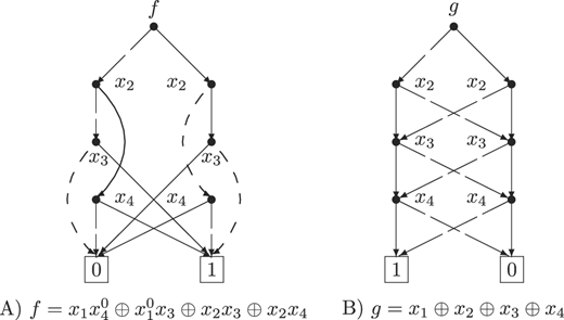
Let and be two Boolean functions. Figure 1 presents their BDDs under the natural variable ordering . All sets of essential variables in g are separable, whereas the sets and are inseparable in f. Clearly, f has non-trivial essential arity gap and Note that the implementations (longest paths) in Figure 1 A) consist of three edges, but in Figure 1 B) of four edges, which shows that the BDD of the function g is extremely complex with respect to the number of its subfunctions and separable sets, whereas the BDD of f is simpler.
3.2 Minor decision diagrams
Next we introduce a new graph-based presentation of the k-valued functions, namely by the minor decision diagrams.
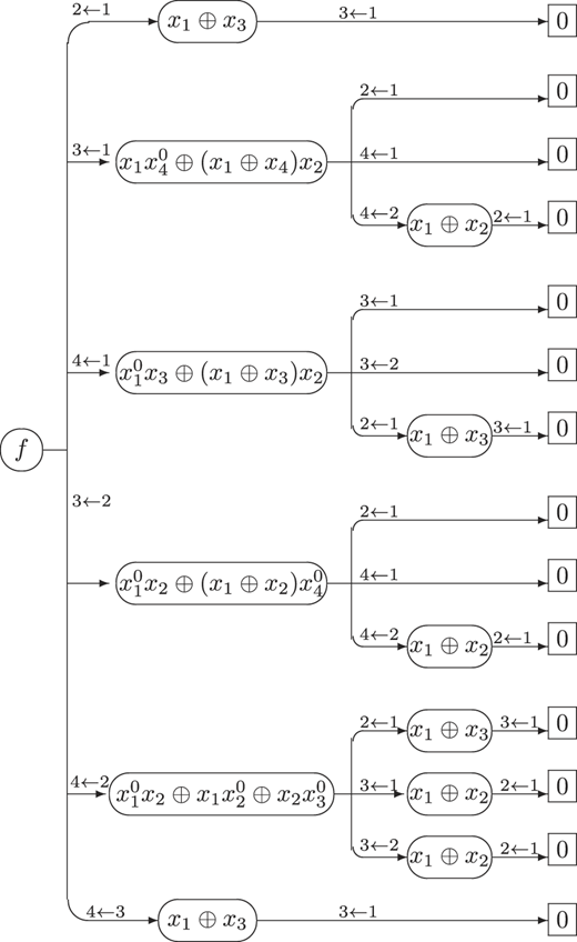
The minor decomposition tree (MDT) of a function, consists of the node, labelled f – called the function node and nodes labelled with minor names, called the internal (non-terminal) nodes, and the rectangular nodes (leaves of the tree) called the terminal nodes. The terminal nodes are labelled with the same name of a function (atomic minor) from (according to Theorem 2.3). The terminal and non-terminal nodes in the MDT for a function f, essentially depending on n variables, are disposed into maximum layers of the tree. The i-th layer consists of names of all the distinct minors of order i, for . Figure 2 presents the MDT of the function , given in Example 3.1.
We introduce the minor decision diagrams (MDDs) for k-valued functions constructed by reducing their minor decomposition trees (MDTs). Let f be a k-valued function. The minor decision diagram (MDD) of f is obtained from the corresponding MDT by reductions of its nodes and edges applying of the following rules, starting from the MDT and continuing until neither rule can be applied:
Reduction rules
If two edges have equivalent (as mappings) labels of their nodes they are merged.
If two nodes have equivalent labels, they are merged.
Let us build the MDDs of the functions from Example 3.1, namely and using the reduction rules and their MDT’s.
Figure 3 A) shows the MDD of the function f, and Figure 3 B) presents the MDD of g. The identification minors of f and g are:
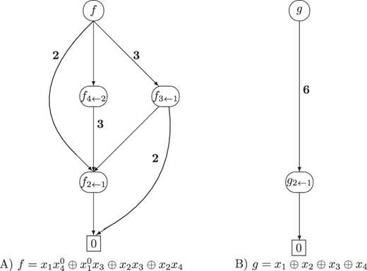
Each edge in the diagram is supplied with a label , (written as bold in Figure 3A), which presents the number of the merged edges of the MDT, connecting the nodes and in MDT.
If two nodes in MDT are connected with unique edge then this edge is presented in MDD without label, for brevity. For example, such pairs are and .
The label of the edge is 3 because there are three identification minors, namely and of f which are equivalent to (see Figure 2).
In a similar way we count the labels of the edges in Figure 3 B).
So, the MDD of f is an acyclic directed graph, with unique function node and according to Theorem 2.3, with unique terminal node. Clearly, the MDD and MDT are uniquely determined by the function f.
3.3 Complexity and equivalence relations with respect to minor reduction
Many of the problems in the applications of the k-valued logic are compounded because of the large number of the functions, namely . Techniques which involve enumeration of functions can only be used if k and n are trivially small. A common way for extending the scope of such enumerative methods is to classify the functions into equivalence classes by some natural equivalence relation.
Let denote the symmetric group of all permutations of the non-empty set A, and let denote the group for a natural number .
A transformation is an n-tuple of k-valued functions acting on a function as follows . Then the composition of two transformations and is defined as follows
The set of all transformations of is the universal monoid with unity - the identical transformation . When taking only invertible transformations we obtain the universal group which is isomorphic to the symmetric group . The groups consisting of invertible transformations of are called transformation groups (sometimes termed permutation groups).
Let be an equivalence relation on the algebra . Since is a finite algebra of k-valued functions, the equivalence relation makes a partition of the algebra in a finite number equivalence classes.
A mapping is called a transformation preserving if for all . Taking only invertible transformations which preserve , we get the group of all transformations preserving . The orbits (also called -types) of this group are denoted by .
Our aim is to classify functions from into equivalence classes by . Thus we have to calculate the number r of -types, to count the number of functions in different equivalence classes, i.e. compute the cardinalities of the sets and to create a list of functions belonging to different -types.
Let and let denote the normal form obtained by applying the reduction on f. According to Theorem 2.3, the normal form is unique and . Thus, our first natural equivalence is defined as follows:
Let f and g be two functions from . We say that f and g are nof-equivalent (written ) if .
The transformation group induced by nof-equivalence is denoted . The transformations in preserve , i.e. for all and . Since the atomic minors (labels of terminal nodes in MDD) depend on at most one essential variable, it follows that the number of the orbits of is equal to . These transformations involve permuting variables, only (see Theorem 3.9, below).
By analogy with the ordered decision diagrams [1,15], we define several equivalence relations in , which allow us to classify the functions by the complexity of their MDDs.
The “scalability” of the diagram is an important measure of the computational complexity of the function. We are going to formalize this problem and establish a method for classification of functions by the minor complexities.
First, the number of all the minors of a function f is a complexity measure, which can be used to evaluate the MDD of f. Namely, it counts the size (number of terminal and non-terminal nodes) of the MDD. M. Couceiro, E. Lehtonen and T. Waldhauser have studied similar evaluation, named “parametrized arity gap” in [5,6], which characterizes the sequential identification minors of a function.
Second, we are going to classify functions in finite algebras under the complexity measures which count the number of minors and the number of ways to obtain these minors.
Let be a k-valued function. Its cmr-complexity is defined as follows:
(i)
(ii)
(iii)
The minors with are excluded because . The minor complexity cmr can be inductively calculated using the MDDs of the functions as it is shown in Example 3.5, given below. We start to assign cmr-complexity equals to 1 for the terminal node, which is labeled by the minor of “0” of highest order according to (i) of Definition 3.4. Next, we inductively calculate the cmr-complexity of the minors of f with lower order, applying (ii) and (iii) of Definition 3.4.
Let us count the cmr-complexity of the function f from Example 3.1 , using the identification minors of f obtained in Example 3.2 and MDD of f, given in Figure 3 A). There is two simple minors of order 2 and four simple minors of order 1. Thus we have and . According to Definition 3.4 we have .
In a similar way from the MDD of g in Figure 3 B) we obtain .
Let f and g be two functions with . We say that f and g are cmr-equivalent (written ) iff:
(i) ;
(ii) there exists a bijection , such that , where , for all , with .
Let denote the transformation group preserving the equivalence , i.e. if and only if .
The nof-equivalence is independent on the cmr-complexity of functions, defined by reduction via minors. For example, the functions and are nof-equivalent, but they are not cmr-equivalent.
Next we define another equivalence based on the number of minors (size of MDD) in a function.
Definition 3.7. Let f and g be two functions from . We say that f and g are mnr-equivalent (written ) if for all .
Clearly, if then . Hence, if then . denotes the transformation group which preserves the equivalence .
Note that do not imply , which can be seen by the following functions: and . Clearly, and , but , and .
(i)
(ii) .
Proof. We argue by induction on the number .
If (basis for induction) then we are clearly done. Assume that (i) and (ii) are satisfied when for some natural number . Let and . Then our inductive assumption implies
and , where and for some and . □
Thus, the complexity is an invariant of the group , and the complexity is an invariant of the group .
It is naturally to ask which groups among “traditional” transformation groups are subgroups of the groups or and which of these groups include as their subgroups.
Let be a mapping and let be a transformation of generated by as follows for all .
The transformation preserves if and only if is a permutation of .
Proof. Let .
First, let be a permutation of . Let be an arbitrary function. If then and we are clearly done. Let and let i and j be two arbitrary natural numbers with . Then we have
Since is a permutation, it follows that which shows that .
Second, let be not a permutation of . Hence, there exist two constants and from such that and . Let be a vector of constants from . Then we define the following function from
Clearly, and the range of f consists of two numbers and . Then , implies that for all . Hence, which shows that and .□
We deal with “natural” equivalence relations which involve variables of functions. Such relations induce permutations of the domain of the functions. These mappings form a transformation group whose number of equivalence classes can be determined. The restricted affine group (RAG) is defined as a subgroup of the symmetric group on the direct sum of the module of arguments of functions and the ring of their outputs. The group RAG permutes the direct sum under restrictions which preserve single-valuedness of all functions from [8,10].
In the model of RAG an affine transformation operates on the domain or space of inputs to produce the output , which might be used as an input in the function f. Its output together with the function variables are linearly combined by a range transformation which defines the image of f as follows:
where d and for are constants from , and . Such a transformation belongs to RAG if is a non-singular matrix.
We want to extract basic facts for several subgroups of RAG which are “neighbourhoods” or “relatives” of our transformation groups .
First, a classification occurs when permuting arguments of functions. If then acts on variables by: . Each permutation generates a map on the domain .
For example, the permutation generates a permutation of the domain of the functions from . Then we have and in cyclic decimal notation this permutation can be written as . The remaining elements of are mapped according to the following cycles of in decimal notation - . Note that each permutation from keeps fixed all k constant tuples from . In case of , these tuples and are presented by the decimal numbers and 26.
denotes the transformation group induced by permuting of variables. Boolean functions of two variables are classified into twelve -classes [8], as it is shown in Table 1. M. Harrison has determined the cycle index of the group . Using Polya’s counting theorem he has counted the number of equivalence classes under permuting arguments (see [8] and Table 3, below).
Number of equivalence classes in under transformation groups.
| N | |||||
|---|---|---|---|---|---|
| 1 | 4 | 2 | 2 | 2 | 2 |
| 2 | 12 | 4 | 3 | 4 | 3 |
| 3 | 80 | 11 | 5 | 11 | 5 |
| 4 | 3984 | ∗ | ∗ | 74 | 11 |
| 5 | 37 333 248 | ∗ | ∗ | ∗ | 38 |
The subgroups of RAG, defined according to (5) which are “relatives” to the groups and are determined as follows: RAG when -non-singular; when ; when ; when ; ; when , where denotes a permutation matrix, is the identity matrix, and are n-dimensional vectors from and .
It is naturally to ask which subgroups of RAG are subgroups of and . Theorem 3.8 shows that and are subgroups of . Clearly, .
Theorem 3.10.
Proof. (i) Follows from Theorem 3.9.(ii) and (iii) – Let and let be a transformation of defined as follows for all . We have to prove that the transformation preserves the equivalence relations and for all . It suffices to show that preserves and . Let be a function and let us assume . It must be shown that and , where for all . Since is a permutation, we have
for all which shows that and hence, . Since and , it follows and .(iv) and (v) – Let and . Then we have and where . Clearly, , and hence and . One can show that there is no transformation , defined as in (5), for which . Consequently, and .(vi), (vii), (viii), (ix) and (xi) – Let and be the functions from . Let
Then clearly, and hence, f and g belong to the same equivalence class under the transformation group . Let . Then we have , which shows that f and g belong to the same equivalence class under the transformation group . One can show that . Example 3.5 shows that . Consequently, and . Theorem 3.8 shows that and . - Let us pick and . Clearly, , but .□
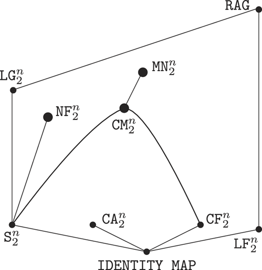
So, Theorem 3.10 summarizes results which determine the positions of the groups and , with respect to the subgroups of RAG. It is well-illustrated by Figure 4, in the case of Boolean functions.
4. Classification of Boolean functions by minor complexities
Table 2 shows the four classes in under the equivalence . The -classes are represented as union of several classes under the permuting arguments, according to Theorem 3.10 (ii), which can be observed in Table 1 and Table 2, given below.
The number of types under permuting arguments, is an upper bound of the number of equivalence classes induced by the relations and (see Figure 4).
In Table 3 the columns named and are calculated in [15] and they present the number of classes under the complexities, determined by the number of subfunctions and separable sets in the functions. It is surprising that for these columns are same as the columns and , i.e. the number of classes are the same, but these classes are very different as sets of functions, determined by these complexities.
Figure 4 presents the subgroups of RAG and transformation groups whose invariants are subfunction, and minor complexities of Boolean functions of n-variables. According to Theorem 3.10 the group has three subgroups from RAG, namely: - the group of permuting arguments, trivial group consisting of the identity map, and - the group of complementing outputs. The groups and are not subgroups of any subgroup of RAG.
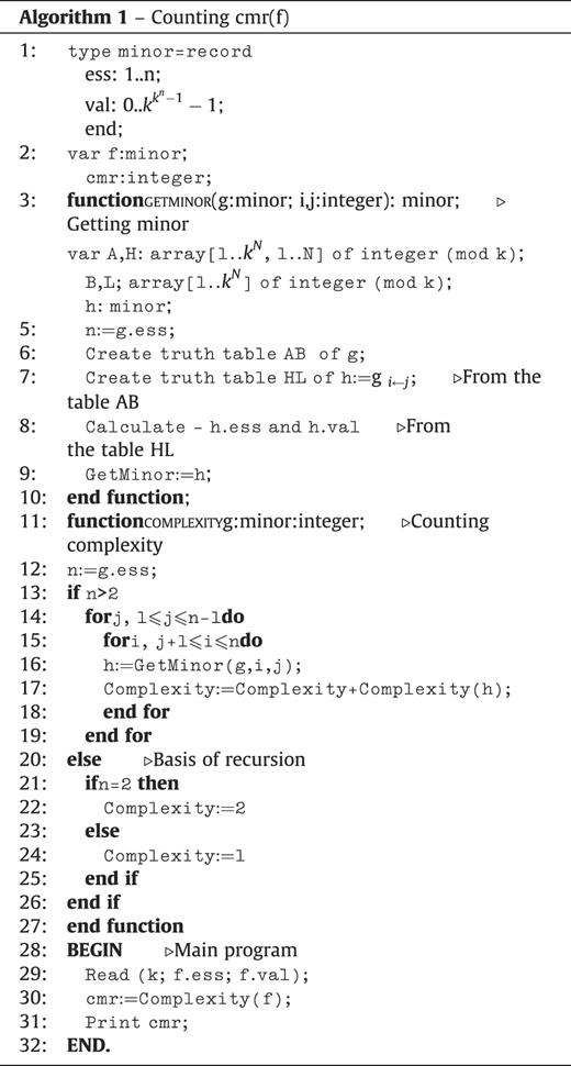
Next, we turn our attention on classifying the functions with respect to their cmr-complexity. This classification is based on the exhaustive Algorithm 1, given below.
Table 4 presents a complete classification of the Boolean functions of tree variables by the minor complexities cmr and mnr. If we agree to regard each 23-tuple as a binary number then the last column presents the vectors of values of all ternary Boolean functions in their table representation with the natural numbers from the set . According to Theorem 3.9, if a natural number , presents a function f which belongs to a cmr-class then the function presented by belongs to the same class. Thus the catalogue contents the numbers , only (see the last column in Table 4). These numbers represent the functions which preserve zero, i.e. the functions f for which . This classification shows that there are eleven equivalence classes under and five classes under .

Theorem 3.8 shows that each mnr-class is a disjoint union of several cmr-classes. Thus the first mnr-class consists of all the functions which belong to the first and the second cmr-class (see fifth column in Table 4). The second mnr-class is equal to the third cmr-class. The fourth and the fifth mnr-classes are unions of three cmr-class, namely: sixth, seventh, and eight, and ninth, tenth, and eleventh, respectively.
The main data structure which describes the nodes in the MDD of f is represented by a record declared as follows:
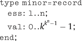
The first field, named ess presents the number of essential variables in the minor (located on the corresponding node) and the second field val is a natural number whose k-ary representation is the last column B of the truth table (of size ) of the minor.
Table 4 presents classification of ternary Boolean functions under the equivalences and , including the catalogue of the equivalence classes (last column). Let us choose a natural number belonging to the seventh column of Table 4, say 24. It belongs to the row numbered 6. The binary representation of 24 is 00011000, because . Hence, the function f corresponding to 24 is evaluated by 1 on the fourth and fifth miniterms, namely and . Consequently, . Then we have and . Clearly, , which is written in the third cell of the sixth row. The MDD of f is shown in the second cell. The cmr-equivalence class containing f consists of 18 functions, according to the fourth cell of the sixth row and the mnr-equivalence class of f contains 108 functions (see whole fifth column of the table). The function is representative for this class (sixth cell). The numerical list of the functions from this equivalence class is given in the last seventh cell of Table 4. The record of the function f is presented as follows f.ess=3 and f.val=24, where k = 2 and B= 00011000.
5. Conclusion
The transformation groups whose invariants are the minor complexities have only three subgroups among the groups in RAG, namely trivial group (identity map), and , whereas the groups whose invariants are the subfunction complexities have three subgroups more (see [15]). One of motivations to study the group is that the reductions are inexpensive and the number of classes is much smaller than the number of classes under the subgroups of RAG, because the order of is so large. As mentioned, the number of equivalence classes under equals to . Hence, the order of is equal to .
The most complex functions with respect to separable sets [15] are grouped in the largest equivalence class. J. Denev and I. Gyudzhenov in [7] proved that for almost all the k-valued functions all the sets of essential variables are separable. Similar results can not be proved for the minor complexities. For example, in the most complex functions belong to the class numbered as 11 (see Table 4), which consists of 16 functions. This class is not so large. It presents 1/16 of the all 256 ternary Boolean functions.
Declarations of interest: None.An idea for a mesure of the minor complexity of functions was presented by M. Couceiro, E. Lehtonen and T. Waldhauser in [5,6], named parametrized arity gap. However, these results, the present paper and [16] are suitable basis for future investigation of the problems for minor complexities and reconstruction of functions from their MDDs.Publishers note: The publisher wishes to inform readers that the article “Minor complexity of discrete functions” was originally published by the previous publisher of Applied Computing and Informatics and the pagination of this article has been subsequently changed. There has been no change to the content of the article. This change was necessary for the journal to transition from the previous publisher to the new one. The publisher sincerely apologises for any inconvenience caused. To access and cite this article, please use Shtrakov, S. (2021), “Minor complexity of discrete functions”, Applied Computing and Informatics. Vol. 17 No. 1, pp. 108-130. The original publication date for this paper was 24/07/2018.

