


Wireless sensor networks (WSNs) are periodically collecting data through randomly dispersed sensors (motes), which typically consume high energy in radio communication that mainly leans on data transmission within the network. Furthermore, dissemination mode in WSN usually produces noisy values, incorrect measurements or missing information that affect the behaviour of WSN. In this article, a Distributed Data Predictive Model (DDPM) was proposed to extend the network lifetime by decreasing the consumption in the energy of sensor nodes. It was built upon a distributive clustering model for predicting dissemination-faults in WSN. The proposed model was developed using Recursive least squares (RLS) adaptive filter integrated with a Finite Impulse Response (FIR) filter, for removing unwanted reflections and noise accompanying of the transferred signals among the sensors, aiming to minimize the size of transferred data for providing energy efficient. The experimental results demonstrated that DDPM reduced the rate of data transmission to ∼20%. Also, it decreased the energy consumption to 95% throughout the dataset sample and upgraded the performance of the sensory network by about 19.5%. Thus, it prolonged the lifetime of the network.
1. Introduction
Wireless Sensor Network (WSN) comprises a Base Station (BS), countless hubs and self-organized tiny devices called sensor nodes. Each sensor encompasses sensing module in which a number of minor sensors, ices, radio- transceiver, restricted battery, memory and microcontroller module which involves Controller Processor Unit (CPU) and Digital Signal Processor (DSP) chipsets. These sensors perform a function in an autonomous manner in the spatial field to get the required values. These sensors are densely deployed and distributed to monitor many ecological conditions, like relative humidity, pressure, temperature, motion, sound pollutants or vibration at different locations. They have to coordinate with each other, to acquire information about the environment. All the aggregated data are transferred to the sink node where valuable data are sorted for managing the vital application. These devices can be deployed for covering some specific domains as reporting the occurrences of any events of interest, aggregation of environmental data, surveillance and target tracking. Although, WSNs have wide applications plentiful gains in battlefield observation, healthcare, weather forecasting and disaster detection [1]. They suffer from redundant transmission and retransmission of network packets in routing, deficient in terms of computation and energy resources. In addition, Sensor networks deploy in inhospitable environments and often need to be adapted to changes in the environmental parameters or users. So, they are requiring to self-awareness and adaptive systems that provide the solution for overcoming the computational complexities, the appearance of transient deployment faults and permanent node failures and suddenly energy sever.
The battery-operated sensors organize themselves according to a certain topology and transmission range for transferring data packets from the source node to traverse multiple hops before they reach terminal. Through WSN communication, thousands of nodes sense the massive volume of data and periodically convey it to a number of hubs; this is resulting in a large amount of data accumulated over a short period and the appearance of many faults through dissemination. Thus, if data dissemination failure occurs at the level of Cluster Head (CH), the aggregate dataset at the head will hold up and CH will emerge a disabled in BS. So, the issue of the huge bulk of datasets produced by these sensors forms a very serious challenge. Further, data communication in WSN consumes a significant amount of energy and occupies a large volume of memory. In order to solve the huge volume of data, we need to solve all the related issues with data dissemination like processing capability and limitation in memory [2]. Although there are limitations facing WSN, WSNs enabled to contribute in various applications and became one of the most vital technologies throughout the recent twenty years. Actually, WSN enables to extend into several zones where a human cannot cover it.
Distributed wireless sensors sense the surrounding events, aggregate them and then disseminate them to the CH. The cluster-head node receives all these data and aggregates it before transferring it to the base station. Therefore, data dissemination is a basic factor in the mission of WSN, while noisy data affect the behaviour of the sensory network. Data diffusion may produce erroneous observed values that may degrade the reliability of the network due to its non-accuracy; also these data are not fully stored due to limited memory. So, several investigators studied energy awareness during data dissemination via routing protocol and considered it as an essential design issue. They depend on the nature of the application and network topology in designing the infrastructure of the network [3]. However, computational and energy resources still represent serious restrictions accompany applications of WSN. The aggregated data often suffer from some inaccuracies and incompleteness [4]. Inaccurate/imperfect measurements in WSN data are often referred to as WSN abnormalities. Abnormalities are defined as the observations that do not correspond to well-defined normal behaviour. Abnormalities, in WSNs, are generated from faults, node malfunctions/failures and attacks. So, it is important to recognize the kind of abnormality to effectively respond.
The efforts in the proposed work (DDPM) were devoted to reducing the rate of data transmission during communication among the nodes in the WSN clusters for conserving the energy. Initially, DDPM emulates elimination the rapid energy depletion and the sudden faults associated with the dissemination operation in WSN. The proposed DDPM encompasses two main paradigms are, 1) Data prediction paradigm: is a dual prediction model built at the cluster head level. During the deployment mode, the distributed sensor nodes disseminate huge data, in form of data packets, at equal time intervals to the head. In case appearance of fault or if the sensed measurements have lost, the cluster head will forecast the missing values based on the historical readings of such sensor nodes. 2) Prediction based-filtering paradigm: enables the model to obtain high convergence of transferred signals. Filtering model refines the signal by removing noise accompanying the transferred signals through integrating two adaptive filters are RLS adaptive filter and FIR filter. The integrated filters were used to allow the sensor nodes to adapt the sensing signals for providing high convergence of the signals. Thus, it will provide a great reduction in power consumption. Finally, methodical evaluation to assess the efficiency of the proposed DDPM, by estimating the rate of data transmission via RMSE and measuring the performance of network using MAPE.
The rest of the research was organized as: Section 2 presents the previous work related to this topic. Section 3 shows problem preliminaries and describes the proposal distributed data- prediction modelling and the suggested algorithm. The evaluation and analytical results are presented in Section 4.
2. Related works
Although WSNs have become the main rate in the field of observation and processing, WSN still suffers from many challenges degrade system accuracy and the life-span quality of any WSN oriented applications. The recent researches exploring advancements in WSN addressed WSN challenges as the problem of energy management, difficulties of achieving efficient processing and communication Patterns. It also reviewed three categories of faults, beyond WSN challenges and misbehaving of WSN are sensor reading faults, software faults and hardware faults [5]. So, the recent techniques exploring solutions for WSN faults and challenges attract a great interest by most of the researchers in the current decade. Generally, the prediction is one of the solutions and it is an essential action to completely provide the estimation of network readings to guarantee the credibility of the network. The prediction techniques that have been implemented and evaluated on different WSN datasets are still insufficient. In this section, the various studies which have been performed regarding the prediction techniques for WSN were mentioned. In 2015, Zhang et al. [6] proposed a dynamic and systematic data reduction approach called DR3. DR3 architecture encompassed three parallel dynamic error control mechanisms to optimize the trade-off between energy saving and data, the mechanism achieves the following 1) Internal Group Data Reduction (IGDR): a centroid node (the selected node according to selection algorithm) will be active through a certain sensing schedule while the remaining sensors are sleeping. The packets associated with originally active nodes will be compressed; 2) Adaptive Lower Duty Cycle Data Reduction (ALDCDR): the centroid node can switch into sleeping status to save its energy. Those patterns can be used for predicting the future outcome by the sensor node; 3) Correlated Group Date Reduction (CGDR): the sensing readings have a high correlation with other groups into sleep status. The sleep sensor group’s sensing reading can be estimated using its correlated group’s reading. Samarah et al. [7] constructed a data prediction model built upon sensor nodes and used the cloud system to generate data. The purpose of the proposed model was, prevent sensor nodes from transferring a large amount of data through deployment cycle and allow to them transferring just differ data than original data (previously the transferred data), hence reduce the energy consumption of the sensor's battery The prediction model was implemented by a line equation through two n-dimensional vectors in n-space. Also, Tan and Wu [8] applied the hierarchical Least-Mean-Square (HLMS) adaptive filter on WSN for forecasting data values between sensor and sink. The adaptive filter was employed at both the sensor and sink, also was used to calculate an identical prediction by using the hierarchical LMS prediction filter rules.
In 2016, Mashere et al. [9] introduced a Controlled Duty Cycle scheme (CDC) based on throttling techniques in WSN. The scheme consisted of threshold level sampling data reduction algorithm and adaptive level sampling data reduction algorithm. The proposed CDC transferred data from a source node through intermediate nodes to the sink node, then select the shortest path for minimizing energy consumption in WSN. Also, Saoudi et al. [10] proposed a new collaborative fire prediction and data reduction method to divide the node set into clusters. Each node can individually detect fires using classification techniques. In 2017, El-Telbany and Maged [11] presented a novel approach hybridized LMS adaptive filter with matrix completion to minimize the necessary information that sensors transmit at WSN. The approach utilized both adaptive filters and matrix completion for WSNs. The importance of approach lies in (i) it deals with limited resources of the sensors, (ii) it allows sensing nodes to adaptively samples the sensed data based on changing the pattern and randomly, (iii) it reconstructs the missing data with excellent precision at the sink which collect the data from sensors. In 2018, Diwakaran et al. [12] introduced a data prediction technique for reducing the amount of data transmission. They discussed decreasing the consumption of energy by filtering to remove the unwanted number of transmission. In this technique, prior knowledge is utilized in predicting the expected values. This was achieved using the Least Mean Square (LMS) algorithm. Fathy et al. [13] propose an Adaptive Method for Data Reduction (AM-DR). The method is a prediction-based data reduction that uses LMS adaptive filters. AM-DR is based on a combination of two coupled LMS filters with differing sizes for estimating the next measured values both at the source and the sink node such that sensor nodes have transmitted only their immediate sensed values that deviate significantly from the predicted values.
3. Distributed data predictive model (DDPM)
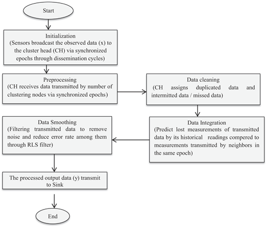
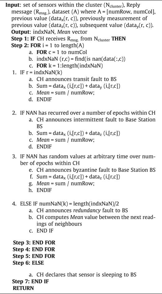
A Distributed Self-Healing Approach (DSHA) mechanism for WSN was previously presented [14]. The investigators succeeded in detecting the defects in hardware components of the sensor node, diagnosing the type of failure as well as applying countermeasures, which included repair of the faulty node by isolating malfunction nodes and topology modification. Generally, the WSN significantly suffers from short lifespan, because of several problems as generating insufficient communication overhead and the sudden faults of deployment operation. Data dissemination is considered the main factor of energy consumption in WSN compared to treatment and detection operations [16]. The present work extended the previous work [14] by introducing a predictive based-filtering model, in order to overcome the challenge of energy resource and problems of the deployment in the designated network. The proposed model (DDPM)significantly reduce the rate of data transmission through predicting the upcoming data and missing readings and then removing the noise associated to the transferred signals, for energy-efficient for WSN, as depicted in the algorithm (1). This model mainly differs in technique and amount of data needed to build the model.
Algorithm (1): The proposed predictive modelling for WSN
3.1 Problem preliminaries
DDPM was based on the studied clustering algorithm in a previous work [14], which was based on Low-energy Adaptive Clustering Hierarchy (LEACH) presented in [15]. In the designing, the proposed sensor network involved in 9 clusters, where each cluster composed of one node represented as a cluster head (CH) and 5 members, which collected a set of measurements related to the atmosphere readings as temperature, humidity and pressure. The proposed DDPM was built upon the following assumptions:
- 1.
Sensor nodes (Si) in the designated network have homogenous characteristics. They report their readings to their cluster head. Also, it has an ID key that expresses its presence inside the group. ID keys are assigned to sensor nodes before deployment mode.
- 2.
Cluster head (CH) was selected by election according to criteria as a battery power (high-energy) and the sum of the distance between the cluster head and other nodes is small. Consequently, the elected CH receives welcome messages from the cluster members and then obtains a list of IDs and respective reply messages continuously. As it directs instructions to the members.
- 3.
VX was referred to a vector of real numbers that represent the sensor readings over a time period.
- 4.
Time was assumed to be divided into a set of equal intervals called time periods (Ti). Ti represents the time periods over the sensor's data stream.
- 5.
VNAN was represented by the missing event and is inferred by observing the following vectors:
- a.
Previous measurements vector of each missing value was represented as:
(3) - b.
subsequent measurements vector of missing value was represented as:
- a.
- 6.
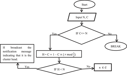
Through the clustering formation, the introduced number of sensor nodes (N) compare with the desired number of cluster heads (H) in each round, by applying the given Eq. (1); if N is less than H, the nodes become CHs, as simplified in the flowchart (1).
where: H is the desired percentage of cluster heads, r is the current round, G is the set of nodes that have not been cluster heads in the last 1/C rounds.
Flowchart (1): The applied clustering algorithm in DDPM
- 7.
The information bearing noisy signal is assumed as a sine wave that is corrupted due to interferences during communication.
3.2 Model description and problem formulation
In an implementation, the proposed modelling (DDPM) scenario was applied as follow:
- A)
Dissemination mode/ Mobility mode: Every node in the cluster transfers observations to the head in form of data packets via reply message that composes of ID node, time and information. Cluster head records the readings of the connected nodes in a reporting list.
- B)
Classification mode: This mode was accomplished at the cluster head level as follows.
- •
If CH did not receive a reply message from Si according to a default timing period throughout one dissemination mode, cluster head will classify that as transit fault and apply Eq. (6) in the generation model.
- •
If sensor node (Si) did not transmit any data to CH in mobility mode throughout a number of epochs, later it transferred data to CH over new epoch, the head will classify that as an intermittent fault and generates Eq. (7).
- •
If the sensor repeats the previous error (do not send any data to the group head) in another dissemination mode among its data transferring intervals, CH will classify them as redundancy fault. This is exemplified in Algorithm (2).
- •
If Si transferred random values at an arbitrary time to CH or stopped broadcasting data, in this case, CH will classify that fault as byzantine. This was illustrated in Eq. (7).
- C)
Data generation mode: The performance of this mode was adequately correlated with sensing session. At the sensor level, certain amounts of data were collected by the sensors present in each cluster throughout the sensing session. Where each node sent the data to the head without making predictions. At the cluster head level, a proper estimation of sensor status was made through this mode. So, if CH did not receive any data from any sensor (Si), it will depend on the historical readings to generate standard values of the missing events (NAN). In the proposed DDPM, generation mode covers two trends are: energy drain trend and non-permanent fault (dissemination fault) trend. To find the missing values (NAN) due to the first trend, DDPM was based on the measurements previously sent by them over near periods of missing period. Then, CH obtained NAN measurement at (t) by computing the mean function of captured measurements at (t−1). Mean function utilized in calculating () was built upon a number of past readings via prior time series (in case, the drain of energy). Finding the mean value of missing event (NAN) due to impermanent fault was built upon the pervious reading at (t−1) and subsequent reading at (t+1). Thus the mechanism performs:
- ■
Absence of a reply message or appearance of a transit fault
- ■
Appearance of intermittent fault & byzantine fault, compute with:
- ■
Occurrence of energy depletion & redundancy fault
By the time, the head node will use neighbouring reading to recover the missing events,
where is the mean measurement of missing event and is continually dependent on time, N is the number of readings involved in generation process and was used to deduce missing event, is the previously data readings and it may be the concluded meant value, is the subsequent reading of missing measurement that used to infer the missing values due to the occurrence of the intermittent error, is the previously measurement of , is the deduced mean value by calculating the formerly measurements at various intervals and was used to locate byzantine the fault.
- D)
Data filtering & modelling mode: in this subsection, the two adaptive filters have integrated to accomplish adaption operation to the transferred signals:
- 1)
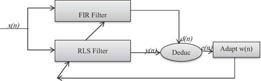
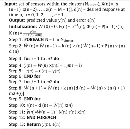
Recursive Least Squares (RLS) is an adaptive filter algorithm that recursively finds the coefficients that minimize a weighted linear least squares cost function relating to the input signals. This approach, in contrast to the least mean squares (LMS), aims to reduce the mean square error. In the derivation of RLS, the input signals of the clustering sensor are considered deterministic. This meant is related to the series of time, in which no randomness is involved in reporting of future readings of the cluster. LMS and similar algorithms are considered stochastic when compared to most of its competitors, where they exhibit extremely fast convergence. RLS algorithm is known for their excellent performance when applied in time-varying environments. In this work, the author tried to develop RLS algorithm, by using the RLS filter integrated with a FIR filter, to reduce error satisfactorily. RLS algorithm estimates the coefficients needed to refine the input signal to obtain the output signal. At the same time, this input signal was converted to the desired signal via FIR adaptive filter for estimating error ratio, see Figure 1. The performance of the RLS algorithm was described in three basic equations as:
where n is the current epoch n, . is the vector of the input samples observed through n, is the vector of filtered weight estimated in epoch n, is the filtered output through n, e(n) is the estimation error in n, d(n) is the desired signal through n. The expansion vector was attained by form:
The filter length is M × M time-average correlation matrix, or the autocorrelation matrix, of inputs vector x (n), x (n−1) …x (n − M + 1). The integrated filter relied on the least square normal equation can be written as:
where z is the M × 1 time-average cross-correlation vector between t inputs x(n), x(n − 1) …x(n − M + 1) and the desired response d(n). The filter weights can be updated at each time n in order to minimize error and is the M × 1 wt vector of the least-squares filter. While, the inverse of the autocorrelation matrix can be computed recursively by P (n) = φ−1 (n), thus:
- ■
is the weight vector can be reformulated so it can be computed recursive:
Substituting −1 (n) using P (n) to become P(n)z(n)
- ■
(n−1) is the “old” value of the correlation matrix and can be applied for z:
Reformulation z (n) using P(n) to obtain (n)1= ʎ P(n) z(n−1) + P(n) × (n) d*(n)
- ■
k(n) is a time varying vector defined as the input vector x(n), altered by φ−1 (n):
- •
Then, P (n) can be computed recursively:
- •
By replacing P (n) for using in (n), to attain
- •
Substituting (n−1) = P (n) z (n), to gain
- •
Then, using k (n) = P (n) × (n), to realize
- •
Hence, using the definition of the estimated error
where: ε is the estimation error, built upon the old weight vector for each iteration.
- 2)
Finite Impulse Response (FIR): is an adaptive filter without fdback, it is also known as non-recursive digital filters, even though recursive algorithms can be used for FIR filter realization. The output y(n) of a filter system idetermined by convolving its input signal x(n) with its impulse response to obtain the desired signal. The output is a weighted sum of the current and a finite number of previous values of the input. In an implementation, the FIR filter used to acquire the desired signal. The operation is described by the following scenario of the FIR filter is as follows:
■ The continuous signal was considered is of the form:
The signals sampled with period T = 1 becomes u(t) = a0 + a1t + a2t + … + amtm. However, the sampled signal with a zero mean noise source e(n) were determined, thus x(n) becomes as the form:
- ■
The value of u(t) with some delay (p) using an FIR filter with the input x(n - N), it can be shown that the optimal impulse response is of the form:
where x(n) is input signal and h(k) is filter coefficients (ci) c0, c1, c2, …,etc. The coefficients (c) are constants depending on the value of (p) and N is a filter order.
- ■
The complexity of the input with a transfer function h[n] provides a filtered output. The mathematical model of the FIR filter is:
where h is a transfer function of an impulse response to the input. The complexity allows the filter to be activated when the input recorded a signal at the same time value.
4. Practical results
To address the studied issue, a dataset of atmospheric changes was handled. The scalar datasets were picked up from 54 sensors. They were deployed in the Intel Berkeley Research lab between February 28th and April 5th (2004). These sensors were reinforced with the stamped topology information along time with humidity, temperature, light and voltage values once recorded every 31 s. The actual data were processed using Matlab tool, Table 1 revealed the notions used later and their explanations:
DDPM notations and their explanations.
| Notation | Explanation |
|---|---|
| Si | The ith member node in the cluster |
| ID | Cluster identifier of sensor nodes belonging to that cluster |
| N | Samples number of the data stream |
| CH | Cluster head/Leader of the group |
| NAN | Missing an event from the sensor in a definite epoch |
| x(n) | A sample of data stream/Input signal at an instant n |
| y(n) | The output signal of the RLS filter |
| w(n) | The weighted signal at an instant n |
| e(n) | The prediction error at an instant n |
| d(n) | The desired signal/Output signal of the FIR filter |
| Predicted value induced from regression | |
| emax | The maximal prediction error value is given at both the source node and terminal node/threshold value |
4.1 Data generation
The longevity of WSN is based on minimization both the rates of transmission and the energy consumption that closely correlated to sensor battery. The lifetime of a node consists of many epochs. Each epoch includes packet transmission time represented as dissemination cycle and sleeps scheduling stage’s execution time, Figure 2. Generally, some sensors may issue the missing events (NAN) through various epochs were assigned by its historical readings. Missing values may be appeared throughout a number of rounds, due to failures, truncated or the sleep schedule.
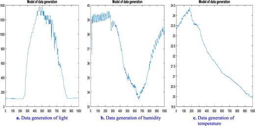
Practically, if a missing event (NAN) has appeared at an arbitrary time, the preceding readings of missing event (NAN) will be set in vector Xi, and then will calculate the mean value among them by CH to infer the lost measurement, see Figure 3. On another hand, CH will depend on the following readings of neighbouring nodes through duty cycle, then it will be assigned in the Xj vector for calculating the mean value between them to represent the value of the missing event, if loss of one sensor data or the missing event has recurred over a number of epochs at a sensor, as illustrated in Table 2. Eqs. (6)–(9) were applied according to the type of missing event as demonstrated in Algorithm (2). It gives samples of a sensor's readings through a programming implementation. Table 3 shows generation process for the missing sample.
Missing data sample through a dissemination cycle.
| Dissemination Cycle | ||||
|---|---|---|---|---|
| Epoch | Sensor _id | temperature | humidity | light |
| 2763 | 4 | 19.9002 | 38.940 | 97.520 |
| 2764 | 4 | 19.9002 | 38.940 | 97.520 |
| 167 | 5 | 2.69964 | NaN | NaN |
| 330 | 5 | 2.67532 | NaN | NaN |
| 525 | 5 | 2.65143 | NaN | NaN |
| 1030 | 5 | 2.65143 | NaN | NaN |
| 1456 | 5 | 2.68742 | NaN | NaN |
| 1483 | 5 | 2.68742 | NaN | NaN |
| 1714 | 5 | 2.67532 | NaN | NaN |
| 1866 | 5 | 2.66332 | NaN | NaN |
| 1918 | 5 | 2.67532 | NaN | NaN |
| 2415 | 5 | 2.62796 | NaN | NaN |
| 2 | 6 | 20.4196 | 36.6118 | 121.44 |
| 6 | 6 | 19.9002 | 37.5737 | 121.44 |
| 22 | 6 | 19.42 | 39.2123 | 121.44 |
| 24 | 6 | 19.42 | 39.0763 | 121.44 |
Prediction for missing events over a dissemination cycle.
| Dissemination Cycle | ||||
|---|---|---|---|---|
| Epoch | Sensor _id | temperature | humidity | Light |
| 2763 | 4 | 19.9002 | 38.940 | 97.520 |
| 2764 | 4 | 19.9002 | 38.940 | 97.520 |
| 167 | 5 | 2.69964 | 37.77595 | 109.4800 |
| 330 | 5 | 2.67532 | 37.77595 | 109.4800 |
| 525 | 5 | 2.65143 | 37.77595 | 109.4800 |
| 1030 | 5 | 2.65143 | 37.77595 | 109.4800 |
| 1456 | 5 | 2.68742 | 37.77595 | 109.4800 |
| 1483 | 5 | 2.68742 | 37.77595 | 109.4800 |
| 1714 | 5 | 2.67532 | 37.77595 | 109.4800 |
| 1866 | 5 | 2.66332 | 37.77595 | 109.4800 |
| 1918 | 5 | 2.67532 | 37.77595 | 109.4800 |
| 2415 | 5 | 2.62796 | 37.77595 | 109.4800 |
| 2 | 6 | 20.4196 | 36.6118 | 121.44 |
| 6 | 6 | 19.9002 | 37.5737 | 121.44 |
| 22 | 6 | 19.42 | 39.2123 | 121.44 |
| 24 | 6 | 19.42 | 39.0763 | 121.44 |
Algorithm (2): Data generation method for finding value missing events
The results in Table 2 show that the sensor nodes have that ids = 4, 5 and 6 transfer data to CH through miscellaneous epochs in a dissemination cycle. Where, CH recorded that the aggregated measurements of humidity and light passing by sensor id = 5 had lost. So, CH starts for classifying the type of fault then predicting the lost events according to Eqs. (6)–(9); the values recorded of these data sector during prediction, are given in Table 3.
It is clear from Table 3 that CH enabled to cover the missing event by taking the mean for the observed historical readings by first-hop neighbouring sensors during the same diffusion cycle. It was worth mentioning that the predicted values that listed in Table 3 relatively converge to the actual values listed in Table 2.
4.2 Data filtering
In this mode, the amount of data transmission rate that delivered to CH was reduced by accomplishing the following sequence:
4.2.1 Filtering signals acquisition stage
In this phase, the integrated adaptive filter was operated at node and head. RLS filter was utilized to extract output signals (y), while FIR filter was used as an inverse system to generate the desired signals (d), see Figure 4. Practically, 1000 temperature samples were picked up and were prepared as input vector (x) taking into consideration the desired signal vector (d), which has the same length as the input signal vector (x) to initialize the processing. The digital signal processing of FIR filter (DSP.FIR) was constructed to filter input (x), for acquiring the desired signal (d) that was manipulated programmatically as:
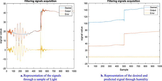
a. Representation of the signals through a sample of Light. b. Representation of the desired and predicted signal through humidity.
a. Representation of the signals through a sample of Light. b. Representation of the desired and predicted signal through humidity.
RLS filter was utilized to refine input signal and obtain the filtered output/ predicted signal (y) along with the error (e) between the reference signal (x) and the desired signal (d), see Figure 4. Throughout each iteration, the proposed adaptive algorithm tried to nominate its coefficients, even error (e) was reduced to as less as possible, by adapting w(n) synchronously as happens in the second phase.
4.2.2 Noise cancellation stage
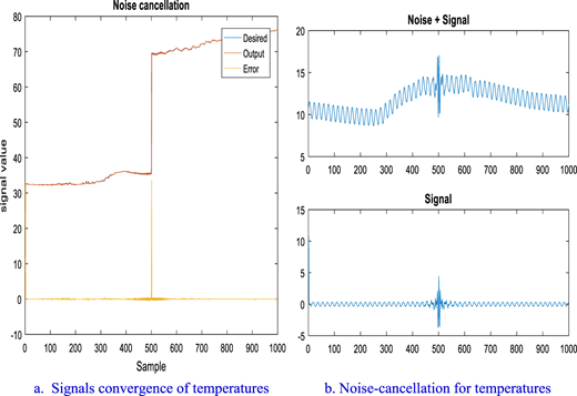
The adaptive systems may insert unwanted signals to a useful signal. So, this phase was developed to cancel any noisy signal or unwanted interference. Generally, a noise represents anything which changes or disrupts a signal as it transmits between a source and destination nodes. In this phase, both FIR and RLS adaptive filters were integrated and applied to refine the signal. In an implementation, the product of w(n) directs into RLS Filter to extract a noise-free output signal, by adjusting the measurement of y(n) with the existing magnitude of w(n) through applying Eq. (8), Algorithm (3). The desired DSP.FIR signal d(n) compares again with the result of DSP.RLS signal y(n) to make sure noise separation by computing e(n) through Eq. (9), also the bit error rate (BER) was calculated by the number of bit errors per unit time. The bit error ratio (BER) is the ratio of the number of errors to the total number of signals sent during a studied time interval and expressed as a percentage, as shown in Table 4. Figure 5-(a) illustrates to converge the output signals from the desired signals, and shrink the ratio of error to almost zero, in the noise cancellation phase. While, Figure 5-(b) shows two subplots; the first subplot demonstrates interference noise and signal, while the second subplot clarifies extracted signal output from the integrated adaptive system.
Noise cancellation of different datasets samples.
| ROUND (4) | ||||
|---|---|---|---|---|
| Temperature | Reference input x(n) | Desired signal d(n) | Output signal y(n) | Error e(n) |
| 23.35 | 23.56 | 23.56 | −0.050 | |
| 23.36 | 23.51 | 23.51 | −3.58 e-05 | |
| 23.38 | 23.53 | 23.53 | −0.036 | |
| 23.34 | 23.46 | 23.46 | 0.072 | |
| 23.36 | 23.55 | 23.55 | −0.036 | |
| 23.35 | 23.50 | 23.50 | 0.018 | |
| 23.36 | 23.53 | 23.51 | −0.018 | |
| 23.35 | 23.51 | 23.50 | 0.018 | |
| 23.40 | 23.56 | 23.56 | −0.073 | |
| 23.44 | 23.54 | 23.54 | −0.0941 | |
| 23.46 | 23.46 | 23.46 | −0.050 | |
| Bit error rate /BER | −0.01937% | |||
| Humidity | Reference input x(n) | Desired signal d(n) | Output signal y(n) | Error e(n) |
|---|---|---|---|---|
| 33.9 | 32.7 | 32.7 | 0.014 | |
| 33.8 | 32.5 | 32.5 | −0.079 | |
| 33.7 | 32.4 | 32.4 | −0.010 | |
| 33.8 | 32.5 | 32.5 | 0.023 | |
| 33.8 | 32.5 | 32.5 | 3.345 e-05 | |
| 33.8 | 32.5 | 32.5 | −0.012 | |
| 33.9 | 32.6 | 32.5 | 0.030 | |
| 34.0 | 32.7 | 32.7 | 0.079 | |
| 33.9 | 32.6 | 32.6 | −0.079 | |
| 33.7 | 32.4 | 32.4 | −0.041 | |
| 33.8 | 32.4 | 32.4 | 0.003 | |
| Bit error rate /BER | −0.00655% | |||
| Light | Reference input x(n) | Desired signal d(n) | Output signal y(n) | Error e(n) |
|---|---|---|---|---|
| 397.44 | 393.409 | 393.407 | 0.0018 | |
| 397.44 | 393.407 | 393.409 | −0.001274 | |
| 397.44 | 393.409 | 393.407 | 0.0019 | |
| 382.72 | 377.996 | 378.839 | −0.8427 | |
| 397.44 | 393.410 | 392.567 | 0.84343 | |
| 397.44 | 393.406 | 393.410 | −0.003897 | |
| 397.44 | 393.411 | 393.406 | 0.0045030 | |
| 397.44 | 393.406 | 393.442 | −0.0362712 | |
| 397.44 | 393.411 | 393.343 | 0.0680422 | |
| 397.44 | 393.405 | 393.443 | −0.0375766 | |
| 397.44 | 393.412 | 393.405 | 0.00710850 | |
| Bit error rate /BER | 0.00046% | |||
Algorithm (3): Distributed data filtering algorithm
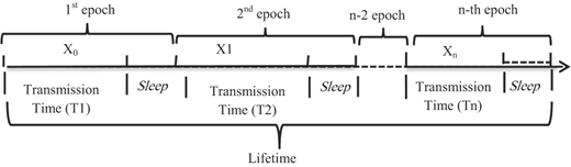
Table 4 demonstrated that the values of BER significantly decreased below zero in the samples of temperatures and humidity through the second paradigm. This demonstrates the purity of the transferred signals from the noise accompanied to it and declares that, the lower the percentage of errors, the better the performance of the system. While the obtained value of BER from the sample of light in such a phase equivalent to zero in the same paradigm. This reveals that the signal may be affected by other interferences such as distortion and poor synchronization.
4.3 Analytical evaluation
The performance and accuracy of prediction were estimated using different evaluation metrics. The used metrics were R-squared (R2), mean absolute percentage error (MAPE), root mean squared error (RMSE), and mean absolute error (MAE):
where the actual measurement as given input; is the filtered output sample value; is the predicted value induced from linear regression between the obtained values of desired and the output and n is the number of measurements.
The error value calculated by subtracting the predicted signal from the desired signal in the root mean square error (RMSE) was selected as a metric for evaluating algorithm performance. Practically, the difference between the desired value and the output value (predicted error) was computed to identify the error (E). The estimation was calculated by the filter for the input signal (x) over time index of each sample. This was done by a linear regression of the combination of readings. The error value was calculated by subtracting the predicted signal from the desired signal, and it was suckled back to adjust the weight (w) of the filter.
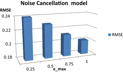
The proposed DDPM reduced the volume of transferred data by each node in the cluster. The data reduction was attained by predicting the upcoming measurement, at the sensor node and destination level, rather than transmitting the data completely. The data will be transmitted only if the predicted value deviates from the original value; under a predefined threshold value, which is a maximal error deviation value and is known as prediction error (emax). The value of emax is given at both source and destination. The sensor nodes do not require to send their actual readings unless there is a deviation (>emax) between the predicted sensor measurements and their actual readings. In this case, the predicted measurement would be included in modelling and will be transmitted to CH. It is worth noting that the researchers in [12] reported that the transmission rate is high when the threshold value (emax) is low. Most researchers also agree that the system is more accurate when the transmission is very low thus producing an energy efficient system. The default 0.25, 0.50, 0.75 and 1.00 were applied throughout implementation. RMSE values were determined according to the values of .
Experimentally, in the signals acquisition phase, RMSE increased when the value of emax increased. While, in the noise cancellation model, the value of RMSE decreased when emax value of the clustering nodes increased. By experiments, evaluation of datasets clarified that RMSE attained the value 0.588 when emax was 0.25, in signals acquisition. With increasing the value of emax up to 1.0, RMSE increased to 0.592. In contrast, MAPE attained a constant value with rising emax to 1.0. In noise cancellation, the value of RMSE decreased from 0.24 to 0.20 when emax increased from 0.25 to 1.0. Contrary, MAPE attained a constant value with the various emax values. This clarified that the amounts of transferred data decrease with increasing emax in this phase. This has prevailed in most samples selected for the experiment. It was worth mentioning that the amount of the transferred original data between the source and destination was very low by the continuous processing, in the noise cancellation model. The obtained results of data reduction were plotted against the specific emax values through cancellation stage in Figure 6 Furthermore, DDPM reinforced the performance quality of the designated network by 19.49%; this raised the creditability of the sensory network. The performance results mentioned in Table 5 below, point out that there is a proportional relationship between data reduction and performance quality, as MAPE increases as the RMSE decreases. It is noticed that the value of MAPE appears 19.4 when RMSE was 0.240 at emax was 0.25, while it goes up to ∼19.5 when the value of RMSE dropped to 0.201 with increasing emax to 1.0. This confirms that the quality depends on data reduction. Additionally, the consumption in energy was directly correlated to the data reduction, where decreasing the data transmission and filtering it significantly save energy. Hence, the proposed model significantly reduced energy consumption and improved sensory network performance. Based on the above, DDPM managed to decrease the amount of the transferred data and improved the performance of the sensory network and contributed efficient-energy, hence raised the quality of the sensory network and prolonged the default lifetime of a sensor node in WSN.
Evaluation of the integrated filter performance through various metrics.
| emax | Signals acquisition | Noise Cancellation | ||||||
|---|---|---|---|---|---|---|---|---|
| RMSE | MAPE | R2 | MAE | RMSE | MAPE | R2 | MAE | |
| 0.25 | 0.588 | 19.357 | 0.218 | 15.7 | 0.240 | 19.4 | 0.769 | 16.6 |
| 0.50 | 0.589 | 19.3568 | 0.419 | 15.8 | 0.229 | 19.45 | 0.858 | 17.4 |
| 0.75 | 0.590 | 19.3569 | 0.520 | 15.9 | 0.212 | 19.47 | 0.905 | 18.4 |
| 1.0 | 0.592 | 19.357 | 0.626 | 16.0 | 0.201 | 19.49 | 0.974 | 18.9 |
Table 5 points out that the best paradigms are the ones that provide the lower RMSE and highest R2 values, also there is relative inversion relationship between data reduction and performance quality, where the values MAPE and MAE increase as the RMSE decreases. It is noticed that the growing value of R2 to 97.8% and low RMSE to 0.20 when emax increased to 1.0, in the phase of noise cancellation. Also, the values of MAE and MAPE continuously go up when RMSE dropped throughout increasing emax level. This confirmed that quality based on data reduction. It can be said that DDPM managed to decrease the rate of data transmission that improved the performance of the sensory network and contributed efficient-energy; hence raised the quality of the sensory network and prolonged the default lifetime of a sensor node in WSN. Also, it accomplished rich-ratio in saving energy getting close to the prediction accuracy ratio.
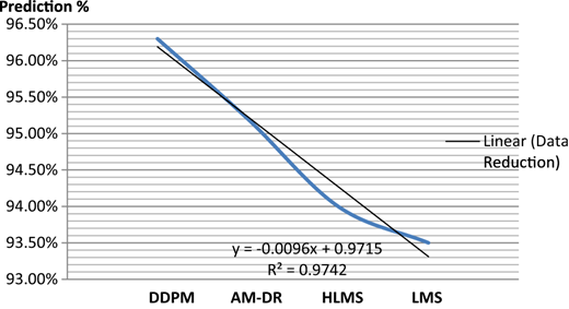
Compared to the state-of-the-art methods, the proposed DDPM decreased data transmission in the cancellation phase to ∼20%, while other researchers [12] have attained a reduction in data transfer up to 35% when emax was 1.0. On another hand, the proposed DDRM achieved ∼96.6% transmission reduction, while AM-DR approach [13] reached ∼95% when emax was 0.5. Also, DDRM accomplished ∼96% transmission reduction when emax was 1.0, while other investigators [12] and [8] attained ∼95% at the same level. DDPM reinforced the performance quality of the designated network by 19.49%; this raised the creditability of the sensory network. It can be said that the proposed DDPM has high predictability for upcoming sensor readings, Figure 7.
4.4 Energy-consumption estimation
The communication energy cost (Ecomm) is a primary key in the estimation of energy consumption. It can be estimated by the operational energy cost of the operational modes (listening, transmission, reception, and sleeping) through the deployment cycle. So, Ecomm can be calculated by:
- 1.
The listening energy (Elisten): refers to the consumed energy when the sensor is active, but not receiving or sending packets.
- 2.
The transmission energy (Et): denotes to the energy consumed during the transmission of packets in active mode. (Et) can be expressed as:
- 3.
The reception energy (Er): indicates to the consumed energy when receiving packets throughout the active state. Er can be stated by:
- 4.
The sleep time (Tslp): demonstrates the energy cost over a duration that has not done within it any operation throughout deployment round.
where Ilisten is the current consumption of the energy in the idle mode and Tlisten is the elapsed time in each epoch by the sensor in listening without sampling or communication. P is a number of the sent bit packets; It is the current consumption of the energy in the transmission mode. PL is the bit length of the packet to be transmitted and Ttb is the transmission time of a bit packet. Ir is the current consumption in a reception mode; PL is the bit length of the packet to be received along, where a node can receive more than one packet during one sampling period and Trb is the reception time of a bit packet. Islp is the current consumption of the energy in the sleep mode and Tslp is the elapsed time in sleep mode within an epoch.
- ■
It can be said that the total energy consumed through communication (Ecomm) or operational energy needed for the operational modes can be calculated as:
- ■
Hence, The energy consumption cost (Econsumption) of the overall system was calculated by energy estimations during communication round and sleep schedule throughout the duty cycle, as:
where P is a total number of the sent bit packets in the active mode; Nactive and Nsleep are the nodes numbers of active and sleep took by the sensor, respectively; Eactive is total the consumed energy in the communication; Tactive and Tsleep are the elapsed times in active and sleep modes, respectively.
As above, during the practical performance, the total energy conservation was estimated in each the round, then in the total duty cycle (see Table 6), as follows:
- 1.
Consumed Energy for the mote (sensor node) in the elapsed epoch:
- 2.
Energy-conservation for the mote:
- 3.
Energy-saving in the deployment rounds, is calculated by:
where E(active, slp) is the consumption energy through either active modes or sleep mode; P is a number of the sent bit packets; PL is the size of the packet estimated by bit, N is the total numbers of the sensor nodes in the round.
Estimation of energy cost was recorded by the clustering sensors for assigning a ratio of energy-saving throughout round 4.
| ROUND (4) | |||||
|---|---|---|---|---|---|
| Cluster (1) | Si1 | Si2 | Si3 | Si4 | Si5 |
| Activation-mode | Active | Active | Active | Active | Sleep |
| Interconnection | communicate | communicate | communicate | communicate | |
| Elapsed time | 3 | 21 | 2 | 15 | 2415 |
| Voltage | 2.69 | 2.68 | 2.69 | 2.65 | 2.69 |
| Consumption-Energy | 0.009 | 0.063 | 0.006 | 0.044 | 0.0005 |
| Energy-conservation | 0.996 | 0.976 | 0.997 | 0.983 | 0.999 |
| Cluster (2) | Si1 | Si2 | Si3 | Si4 | Si5 |
| Activation-mode | Active | Active | Active | Active | Active |
| Interconnection | communicate | communicate | communicate | communicate | communicate |
| Elapsed time | 15 | 9 | 15 | 6 | 9 |
| Voltage | 2.68 | 2.68 | 2.77 | 2.67 | 2.68 |
| Consumption-Energy | 0.045 | 0.0267 | 0.046 | 0.0178 | 0.0266 |
| Energy-conservation | 0.983 | 0.990 | 0.983 | 0.993 | 0.990 |
| Cluster (3) | Si1 | Si2 | Si3 | Si4 | Si5 |
| Activation-mode | Active | Active | Sleep | Active | Active |
| Interconnection | communicate | communicate | communicate | communicate | |
| Elapsed time | 30 | 16 | 3113 | 8 | 2 |
| Voltage | 2.65 | 2.69 | 2.69 | 2.62 | 2.52 |
| Consumption-Energy | 0.088 | 0.047 | 0.00069 | 0.023 | 0.0056 |
| Energy-conservation | 0.967 | 0.982 | 0.9997 | 0.991 | 0.997 |
| Cluster (4) | Si1 | Si2 | Si3 | Si4 | Si5 |
| Activation-mode | Active | Active | Active | Active | Active |
| Interconnection | communicate | communicate | communicate | communicate | communicate |
| Elapsed time | 2 | 2 | 7 | 3 | 3 |
| Voltage | 2.69 | 2.90 | 2.69 | 2.65 | 2.69 |
| Consumption-Energy | 0.006 | 0.007 | 0.020 | 0.009 | 0.009 |
| Energy-conservation | 0.996 | 0.997 | 0.992 | 0.996 | 0.996 |
| Cluster (5) | Si1 | Si2 | Si3 | Si4 | Si5 |
| Activation-mode | Active | Active | Active | Active | Sleep |
| Interconnection | communicate | communicate | communicate | communicate | |
| Elapsed time | 2 | 22 | 300 | 10 | 3602 |
| Voltage | 2.69 | 1.97 | 2.08 | 2.69 | 2.69 |
| Consumption-Energy | 0.00597 | 0.048 | 0.693 | 0.029 | 0.00080 |
| Energy-conservation | 0.997 | 0.975 | 0.667 | 0.988 | 0.9997 |
| Cluster (6) | Si1 | Si2 | Si3 | Si4 | Si5 |
| Activation-mode | Sleep | Active | Sleep | Active | Active |
| Interconnection | communicate | communicate | communicate | ||
| Elapsed time | 830 | 46 | 3638 | 149 | 510 |
| Voltage | 2.68 | 2.78 | 2.47 | 2.128 | 2.46 |
| Consumption-Energy | 0.00018 | 0.142 | 0.00074 | 0.352 | 1.39 |
| Energy-conservation | 0.999 | 0.948 | 0.999 | 0.834 | 0.433 |
| Cluster (7) | Si1 | Si2 | Si3 | Si4 | Si5 |
| Activation-mode | Sleep | Active | Active | Active | Sleep |
| Interconnection | communicate | communicate | communicate | ||
| Elapsed time | 1512 | 467 | 526 | 36 | 3630 |
| Voltage | 2.167 | 2.65 | 2.15 | 2.56 | 2.49 |
| Consumption-Energy | 0.00027 | 1.375 | 1.256 | 0.1024 | 0.00075 |
| Energy-conservation | 0.999 | 0.481 | 0.415 | 0.96 | 0.999 |
| Cluster (8) | Si1 | Si2 | Si3 | Si4 | Si5 |
| Activation-mode | Active | Active | Active | Active | Active |
| Interconnection | communicate | communicate | communicate | communicate | communicate |
| Elapsed time | 253 | 552 | 357 | 252 | 4 |
| Voltage | 2.35 | 2.32 | 2.33 | 2.25 | 2.38 |
| Consumption-Energy | 0.660 | 1.422 | 0.924 | 0.36 | 0.01 |
| Energy-conservation | 0.718 | 0.897 | 0.603 | 0.72 | 0.995 |
| Cluster (9) | Si1 | Si2 | Si3 | Si4 | Si5 |
| Activation-mode | Active | Active | Active | Active | Active |
| Interconnection | communicate | communicate | communicate | communicate | communicate |
| Elapsed time | 58 | 307 | 248 | 375 | 70 |
| Voltage | 2.17 | 2.14 | 2.05 | 2.01 | 2.23 |
| Consumption-Energy | 0.139 | 0.729 | 0.564 | 0.8375 | 0.173 |
| Energy-conservation | 0.935 | 0.658 | 0.724 | 0.583 | 0.922 |
| Energy-saving in the Round | 89. 5% | ||||
5. Conclusion
In this study, a proposed distributed data prediction model (DDPM) was applied to a real-world temperature dataset. These real set suffer from noisy measurements and often lost values. The model was applied to predict the upcoming measurements and recover the missing readings of sensor that resulted from diffusion faults and sleep schedule. Then, it filtered these measurements to refine the transferred signals aimed to significantly energy efficient. The proposed model was built upon a combination of two adaptive filters are RLS and FIR at both source and destination levels. It aimed to get rid of the noise associating to signal values. The filtering was implemented through two phases are, signals acquisition phase and noise cancellation phase. The results clarified that the data generation algorithm recovered ∼99% of lost data in observation and deployment fields. The distributed filtering algorithm had reduced data transmission to 96.6% when emax was 0.5, while retained about 96% with a deviation of the picked real-datasets when emax was 1.0, thus it provided ∼95% of energy throughout the selected sample. Both prediction and filtering processes significantly reduced the volume of transmitted signals, minimized the energy consumption, improved sensory network performance and ensured high reliability estimated by 19% for the designed WSN. In future, experimental efforts will extend to maintain the confidentiality of the sensory network based upon data aggregation.
Publishers note: The publisher wishes to inform readers that the article “Integrated data reduction model in wireless sensor networks” was originally published by the previous publisher of Applied Computing and Informatics and the pagination of this article has been subsequently changed. There has been no change to the content of the article. This change was necessary for the journal to transition from the previous publisher to the new one. The publisher sincerely apologises for any inconvenience caused. To access and cite this article, please use El-Sayed, W.M., El-Bakry, H.M., El-Sayed, S.M. (2020), “Integrated data reduction model in wireless sensor networks”, Applied Computing and Informatics. Vol. ahead-of-print No. ahead-of-print. https://10.1016/j.aci.2019.03.003. The original publication date for this paper was 15/04/2019.

