


Neural networks are used in diverse applications, making them vulnerable to tampering and reinforcing the need for ownership authentication. The proposed method is based on a steganographic technique that embeds binary information into the weights using the IEEE 754 representation to enhance the security of the neural network and ownership authentication.
The proposed method is assessed using a variational autoencoder. Moreover, this technique can be extended to other neural networks. Ownership information is embedded within the most stable layers of the neural network, determined via gradient-based analysis, to enhance robustness against common model alterations, including fine-tuning, compression, pruning, overwriting, noise injection and weight quantization.
The experimental results confirm minimal impact on model performance and ensure reliable data recovery. The bit error rate evaluates the robustness of the proposed method, which obtained values ranging from 0.0131 to 0.129 for different weight pruning (10–50%). These results were further corroborated by extensive experimental validation.
The proposed method introduces a steganographic technique that embeds ownership information using the IEEE 754 representation. Unlike existing techniques, this approach embeds information into the weights without modifying the model structure and maintains the model’s performance without structural changes.
1. Introduction
With the rapid development and widespread application of artificial intelligence (AI) systems based on neural networks, the need for robust intellectual property protection has become critical. Therefore, reliable ownership authentication methods are designed to prevent unauthorized use and tampering [1–4]. Different protection methodologies have been proposed, including steganography, watermarking, fingerprinting and backdoor-based verifications, offering copyright protection, enabling ownership verification and supporting authentication [5–9]. White-box protection methods embed information into the parameters of a neural network to verify ownership. Often, these techniques require access to the neural network parameters to ensure intellectual property protection and ownership verification of neural networks [10–13]. Protecting neural networks against pruning and compression remains a critical research area, as these techniques reduce model size and computational cost.
Recent methods have aimed to preserve model accuracy while embedding ownership information. Watermark embedding during training enhance protection effectiveness while maintaining model accuracy. However, retraining the network may remove the watermark [14]. Ownership data embedding on the discrete cosine transform (DCT) coefficients enhances resistance to pruning without affecting accuracy. However, it has limited payload embedding capacity [15]. Multi-watermark embedding has been demonstrated to have a minimal impact on model performance, and it is designed for robust information hiding. The watermark extraction may be computationally intensive [16]. Hybrid methods use zero-watermarking bit and neural network optimization as a second watermarking layer to enhance robustness. This makes it difficult to balance robustness, imperceptibility and efficiency [17]. The parameter regularizer function for embedding during training or fine-tuning allows data embedding across training. Its robustness is limited to certain attacks [18]. White-box feature embedding via decision tree selection enables relevant feature selection for embedding control. However, it is vulnerable to model extraction attacks [19]. The implementation of the Power Function Mapping (PF-Mapping) as an activation function embeds information with a secret key, but it is vulnerable to pruning [20]. DCT middle frequency coefficients replacement maintains the classification accuracy. The method has limited payload embedding [21]. Kernel information embedding generates robustness against fine-tuning and pruning. It requires high computational processing [22]. The protection of neural networks using layers is achieved through keys that modify the parameters, enabling multiple verification checks. If these layers are removed, model performance decreases [23]. ChainMarks embeds watermarks using cryptographic sequences for ownership verification even if the model has been modified or retrained. However, it creates a dependency on the original data [24]. Most methods focus on embedding information in the neural network parameters and assess performance based on the original task.
The proposed method enhances the robustness of neural networks against pruning, fine-tuning, overwriting and quantization attacks by embedding binary ownership information into the model weights. This is achieved through a steganographic bit replacement technique (15th bit) using the IEEE 754 floating-point representation to modify specific bits without affecting the performance. This approach was implemented in a variational autoencoder (VAE), but it is generalizable to other architectures. To minimize performance degradation, ownership information is embedded in stable layers with low gradient magnitudes, as these layers are less sensitive to small parameter changes. Experimental results demonstrate that the embedding process is imperceptible in terms of accuracy loss and robustness against optimization attacks. The main contributions are:
The bit replacement technique is used for the binary ownership information embedding into neural network weights, ensuring imperceptibility and preserving the model performance.
The incorporation of the IEEE 754 standard ensures that the embedded information remains undetectable and can be recovered for neural network ownership verification.
The combination of IEEE 754 representation and the 15th bit replacement from the selected weight value improves the robustness against attacks, including fine-tuning, pruning and parameter overwriting.
Gradient analysis identifies stable layers to enhance security and robustness against structural optimizations of the model and unauthorized tampering.
This methodology contributes to neural network security by introducing a robust and efficient steganographic framework for intellectual property protection.
2. Methods
The proposed method embeds a binary sequence into the weights by modifying specific bits in their IEEE 754 representation, enabling imperceptible ownership information. During authentication, the embedded sequence is retrieved to verify model ownership.
Figure 1 illustrates the data embedding and extraction process. A VAE is employed to demonstrate the effectiveness of the proposed method, preserving its performance by reconstructing the original image in case of tampering.
 The figure presents the complete workflow for neural network protection, authentication, and performance evaluation based on a variational autoencoder (V A E). The process starts with an image dataset O subscript k, where each image is resized to 128 × 128 pixels before being processed by the encoder. The encoder consists of consecutive layers with 32, 64, 128, 256, 512, and 1024 neurons, which progressively extract feature representations. The encoder output is mapped into a latent space through a reparameterization operation defined as z=μ+σϵ. The latent representation is then passed to the decoder, which reconstructs the images using layers with 1024, 512, 256, 128, 64, 32, and 3 neurons, enabling image reconstruction for performance evaluation of the model. In parallel, encoder weight extraction is performed using the average gradient of each layer to identify the most stable layers. The selected weights are converted into their I E E E 754 floating-point binary representation. For neural network protection, a binary watermark is embedded by replacing the 15th bit of each selected weight. The modified binary values are then converted back to decimal form and reintegrated into the encoder, producing modified encoder weights. For neural network authentication, the same stable layer selection and I E E E 754 conversion process is applied to extract the embedded watermark from the 15th bit of the selected weights. The extracted binary sequence is compared with the original watermark to verify model ownership and integrity.
 Binary sequence embedding and extraction from neural network weights for model authentication
The figure presents the complete workflow for neural network protection, authentication, and performance evaluation based on a variational autoencoder (V A E). The process starts with an image dataset O subscript k, where each image is resized to 128 × 128 pixels before being processed by the encoder. The encoder consists of consecutive layers with 32, 64, 128, 256, 512, and 1024 neurons, which progressively extract feature representations. The encoder output is mapped into a latent space through a reparameterization operation defined as z=μ+σϵ. The latent representation is then passed to the decoder, which reconstructs the images using layers with 1024, 512, 256, 128, 64, 32, and 3 neurons, enabling image reconstruction for performance evaluation of the model. In parallel, encoder weight extraction is performed using the average gradient of each layer to identify the most stable layers. The selected weights are converted into their I E E E 754 floating-point binary representation. For neural network protection, a binary watermark is embedded by replacing the 15th bit of each selected weight. The modified binary values are then converted back to decimal form and reintegrated into the encoder, producing modified encoder weights. For neural network authentication, the same stable layer selection and I E E E 754 conversion process is applied to extract the embedded watermark from the 15th bit of the selected weights. The extracted binary sequence is compared with the original watermark to verify model ownership and integrity. Binary sequence embedding and extraction from neural network weights for model authentication
2.1 Weights extraction and selection
The weights from stable layers are selected to embed the binary sequence by modifying specific bits of each one on its IEEE 754 floating representation [25]. The selection of stable layers minimizes the performance degradation of the neural network and improves the robustness of the model against manipulations. Layer stability is estimated by analyzing the gradient magnitudes, where lower values indicate more stability. The gradient measures how a parameter (weight or bias) changes. For a given weight and a dataset , k = 1, …, L, the gradient is defined as (1):
The model parameters were updated during training by using the gradient descent algorithm (2) to minimize the loss function.
where η is the learning rate and w is updated () with gradient descent. Therefore, the average gradient magnitude is computed across the dataset, which is calculated as (3):
After calculating the gradient magnitude, a list containing each layer (layer) and the corresponding average gradient magnitude, , is generated. This list is sorted by SG in ascending order () according to the values to identify the most stable layers (4):
The first four layers in SG with the smallest gradients were selected to embed binary information. This strategy improves robustness since these stable layers are less susceptible to fine-tuning. Then, the weight tensor from encoder (5) is extracted to embed the binary information on the stable layers.
where i and j are the index of the layer and the neuron, respectively. Therefore, the binary sequence was embedded in the neural network weights, using the bit-replacement steganography method.
Figure 2 presents the pseudocode steps to illustrate the selection of the stable weights procedure employed during the embedding process.
 Figure 2 illustrates the algorithm used to select stable weight parameters from a trained neural network model. The input to the algorithm is the set of trained weight parameters w obtained from model M, and the output is the set of selected stable encoder weights W subscript E. The process begins by initializing a list S subscript G to store the average gradient values of each layer. For each weight node in the model, the gradient is computed. Then, for each layer in the model over the dataset O subscript k, the average gradient magnitude G subscript k is calculated and stored together with the corresponding layer index in S subscript G. The list S subscript G is subsequently sorted in ascending order according to the average gradient magnitude, allowing the layers with the smallest gradient values to be identified as the most stable. The first N layers with the lowest G subscript k values are selected. Finally, the weight parameters corresponding to the selected stable layers are extracted from the encoder and stored in the set W subscript E, which is returned as the output of the algorithm.
Pseudocode for stable weights selection
Figure 2 illustrates the algorithm used to select stable weight parameters from a trained neural network model. The input to the algorithm is the set of trained weight parameters w obtained from model M, and the output is the set of selected stable encoder weights W subscript E. The process begins by initializing a list S subscript G to store the average gradient values of each layer. For each weight node in the model, the gradient is computed. Then, for each layer in the model over the dataset O subscript k, the average gradient magnitude G subscript k is calculated and stored together with the corresponding layer index in S subscript G. The list S subscript G is subsequently sorted in ascending order according to the average gradient magnitude, allowing the layers with the smallest gradient values to be identified as the most stable. The first N layers with the lowest G subscript k values are selected. Finally, the weight parameters corresponding to the selected stable layers are extracted from the encoder and stored in the set W subscript E, which is returned as the output of the algorithm.Pseudocode for stable weights selection
2.2 Steganography 15th bit-replacement on the neural network weights
Ownership information is embedded in the neural network by replacing the 15th bit of the IEEE 754 floating-point representation in its 32-bit format to encode the watermark. The IEEE 754 format increases security and minimizes perceptibility. This format transforms each floating-point number into its binary representation using three components (6): (1) Sign (S, 1 bit), (2) Exponent (E, 8 bits) and (3) Mantissa (M, 23 bits).
The Sign (S) indicate whether the number is positive or negative, represented by the most significant bit (MSB) (7):
The Exponent (E) defines the magnitude of the represented number. In the 32-bit format, the exponent is stored in 8 bits. For example, the binary number 1000.012 can be normalized and represented as: 1.0000 x, E = 3. Therefore, the stored exponent value is computed as (8) by adding a bias of 127, which is specific to the 32-bit floating-point format of the IEEE 754 representation.
The Mantissa (M) represents the fractional part of a decimal number. This element consists of 23 bits denoted as , where each , and it is expressed as (9):
This binary representation is obtained through the following process: 1) Multiply the fractional part by 2. 2) The integer part of the result becomes the next bit. 3) The remaining fractional part is used for the next iteration. For example, for 0.75 in binary: Step 1: 0.75 × 2 = 1.5, integer part = 1 (first bit), fractional part = 0.5. Step 2: 0.5 × 2 = 1.0, integer part = 1 (second bit) and fractional part = 0. Conversion ends since the fractional part is zero. The binary representation of 0.75 is 0.112. Therefore, the Mantissa is M = 11,000…0 (21 zeros added to complete 23 bits).
Once the IEEE 754 representation of the weights is obtained, the 15th bit is modified with the binary sequence (10). The 15th bit was selected because its modification has a minimal impact on the performance of the model.
where l is the corresponding bit from the binary sequence . Therefore, the modified weights are converted to their decimal representations. The recovery of the original decimal values from the IEEE 754 representation involves extracting the sign bit (11), exponent E’ (12) and mantissa (13), with the final value computed using (14):
where is the bit sign (0 = positive, 1 = negative), is the decimal value from the stored exponent, is the decimal value from the Mantissa M and X denotes the value of the number in decimal obtained from its IEEE 754 representation. Finally, the weights parameters were restored to their decimal forms.
Figure 3 illustrates the pseudocode of the watermark embedding process, detailing the steps required to integrate the binary sequence into the selected stable weights.
 Figure 3 illustrates the algorithm used to embed a binary watermark into the stable weight parameters of the neural network. The input to the algorithm is the set of stable encoder weights W subscript E, and the output is the set of modified weight parameters. For each weight in W subscript E, the weight is first converted into its I E E E 754 floating-point binary representation. A binary watermark bit is then embedded by replacing the 15th bit of the I E E E 754 representation with the corresponding watermark bit. After the bit replacement, the modified binary weight is converted back into its decimal floating-point representation. Finally, each original stable weight is updated with its corresponding modified decimal value, resulting in the watermarked weight set.
Pseudocode for watermark embedding
Figure 3 illustrates the algorithm used to embed a binary watermark into the stable weight parameters of the neural network. The input to the algorithm is the set of stable encoder weights W subscript E, and the output is the set of modified weight parameters. For each weight in W subscript E, the weight is first converted into its I E E E 754 floating-point binary representation. A binary watermark bit is then embedded by replacing the 15th bit of the I E E E 754 representation with the corresponding watermark bit. After the bit replacement, the modified binary weight is converted back into its decimal floating-point representation. Finally, each original stable weight is updated with its corresponding modified decimal value, resulting in the watermarked weight set.Pseudocode for watermark embedding
2.3 Ownership authentication of deep learning models
The ownership authentication protects against unauthorized use, ensuring the integrity of the model by extracting the embedded information into the weight parameters from the neural network.
First, it is necessary to locate the modified by calculating the gradient to identify the most stable layers. During verification, the gradients are recalculated to accurately locate these stable layers. For this reason, the authentication process uses the modified weight tensor (15), which is converted to IEEE 754 format to extract the embedded sequence using in (16), using (6)-(8).
Therefore, the 15th bit of each weight in the IEEE 754 representation is extracted to recover the embedded binary information , (17), which is used to verify the authenticity of the model.
The authentication process verifies the ownership of the neural network by retrieving the embedded information. Furthermore, the proposed method preserves the model accuracy and provides a secure methodology for intellectual property protection.
Figure 4 presents the pseudocode for watermark retrieval, showing the procedure used to extract the embedded binary sequence from the stable weights.
 Figure 4 illustrates the algorithm used to retrieve the embedded binary watermark from the modified stable weight parameters of the neural network. The input to the algorithm is the set of modified stable weights WME, and the output is the retrieved watermark sequence. For each weight in W subscript ME, the weight is converted into its I E E E 754 floating-point binary representation. The watermark retrieval process consists of extracting the 15th bit from each binary weight representation. The extracted bits are collected sequentially to form the retrieved watermark s subscript br, which is returned as the output of the algorithm and used for neural network authentication.
Pseudocode for watermark retrieval
Figure 4 illustrates the algorithm used to retrieve the embedded binary watermark from the modified stable weight parameters of the neural network. The input to the algorithm is the set of modified stable weights WME, and the output is the retrieved watermark sequence. For each weight in W subscript ME, the weight is converted into its I E E E 754 floating-point binary representation. The watermark retrieval process consists of extracting the 15th bit from each binary weight representation. The extracted bits are collected sequentially to form the retrieved watermark s subscript br, which is returned as the output of the algorithm and used for neural network authentication.Pseudocode for watermark retrieval
3. Results
This section presents the validation of the robustness against attacks such as quantization, pruning, fine-tuning, and noise injection. In addition, the VAE performance was assessed under image forgery scenarios involving object addition and removal. For evaluation, the MICC-F220 [26], coverage [27], realistic tampering [28] and a proprietary dataset were employed to provide a comprehensive assessment. Results demonstrate that the proposed method preserves the performance of the neural network even when the weights are modified. The algorithm was implemented in Python with PyTorch and executed on a system with a NVIDIA GeForce-4050 GPU and an Intel-CoreUltra-7 processor.
3.1 Neural network performance with modified weights (image reconstruction)
The neural network performance was evaluated by comparing the quality of the reconstructed image against the original image. PSNR measures the ratio between the original image and the noise in the reconstructed image (18).
where MSE is the mean squared error (19).
R and C denote the number of rows and columns and (x, y) the pixel coordinates. In contrast, SSIM evaluates image quality based on luminance, texture and structural similarity (20).
where represent the mean values, are the image variances and is the covariance. Finally, and are constant A higher SSIM indicates structural similarity between the reconstructed and original images.
Table 1 shows that the reconstruction of manipulated images using the neural network with modified weights is comparable to the performance of models with unmodified weights, as it is reflected in the PSNR and SSIM values.
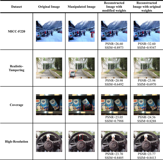
Figure 5 compares the image reconstruction accuracy for 20 random images. This comparison shows that SSIM values from the modified and the original model are similar, demonstrating that embedding information has minimal impact on reconstruction quality.
 Figure 5 presents a comparison of the S S I M between neural networks using original weights and networks using modified (watermarked) weights across four different image databases. In all graphs, the horizontal axis represents the number of images used for evaluation, while the vertical axis represents the S S I M value. Each graph includes two curves: a solid line corresponding to the modified weights and a dashed line corresponding to the original weights. All evaluations are performed using 20 images. Graph (a), corresponding to the M I C C-F220 database, shows relatively stable S S I M values for both configurations, with the modified weights maintaining S S I M values around 0.80, while the original weights consistently achieve higher S S I M values close to 0.90. Graph (b), corresponding to the Realistic Tampering database, exhibits noticeable fluctuations in S S I M values. Both modified and original weights show variations across the evaluated images, with S S I M values decreasing toward the end of the evaluation. Graph (c), corresponding to the Coverage database, shows similar fluctuation patterns for both modified and original weights, with S S I M values ranging from mid to high levels. A slight decrease is observed for the original weights at higher image counts. Graph (d), corresponding to the High-Resolution database, demonstrates the largest variation in S S I M values. The modified weights exhibit a wide range of S S I M values, while the original weights show both flat regions and sharper decreases at specific image counts. Overall, the figure illustrates that the use of modified weights for watermark embedding preserves acceptable image reconstruction quality while maintaining S S I M behavior comparable to that of the original network across different datasets.
SSIM comparison of reconstructed images using original and modified VAE weights: (a) SSIM MICC-F220, (b) SSIM realistic tampering, (c) SSIM coverage and (d) SSIM high resolution
Figure 5 presents a comparison of the S S I M between neural networks using original weights and networks using modified (watermarked) weights across four different image databases. In all graphs, the horizontal axis represents the number of images used for evaluation, while the vertical axis represents the S S I M value. Each graph includes two curves: a solid line corresponding to the modified weights and a dashed line corresponding to the original weights. All evaluations are performed using 20 images. Graph (a), corresponding to the M I C C-F220 database, shows relatively stable S S I M values for both configurations, with the modified weights maintaining S S I M values around 0.80, while the original weights consistently achieve higher S S I M values close to 0.90. Graph (b), corresponding to the Realistic Tampering database, exhibits noticeable fluctuations in S S I M values. Both modified and original weights show variations across the evaluated images, with S S I M values decreasing toward the end of the evaluation. Graph (c), corresponding to the Coverage database, shows similar fluctuation patterns for both modified and original weights, with S S I M values ranging from mid to high levels. A slight decrease is observed for the original weights at higher image counts. Graph (d), corresponding to the High-Resolution database, demonstrates the largest variation in S S I M values. The modified weights exhibit a wide range of S S I M values, while the original weights show both flat regions and sharper decreases at specific image counts. Overall, the figure illustrates that the use of modified weights for watermark embedding preserves acceptable image reconstruction quality while maintaining S S I M behavior comparable to that of the original network across different datasets.SSIM comparison of reconstructed images using original and modified VAE weights: (a) SSIM MICC-F220, (b) SSIM realistic tampering, (c) SSIM coverage and (d) SSIM high resolution
Figure 6 presents the processing time required for the recovery of the embedded information and image reconstruction. Images from the high-resolution dataset need more processing time during processing and reconstruction for their size.
 Figure 6 presents a comparison of the authentication and image reconstruction processing time of the proposed neural network across different image databases. The horizontal axis represents the number of images used in the evaluation, while the vertical axis represents the processing time in seconds. Each curve corresponds to a different dataset, including M I C C-F220, Realistic Tampering, Coverage, and High-Resolution databases. The High-Resolution database exhibits the highest and most consistent processing time across all evaluated image counts, reflecting the increased computational complexity associated with higher-resolution images. In contrast, the M I C C-F220 database shows the lowest processing times, remaining close to a constant value with only a slight increase at higher image counts. The Realistic Tampering and Coverage databases present moderate processing times, with occasional peaks indicating increased computational demand during authentication and image reconstruction. Despite these fluctuations, the overall processing time remains within a narrow range for all datasets. Overall, the figure demonstrates that the proposed neural network maintains efficient and scalable performance across different databases, even when processing images of varying complexity and resolution.
Processing time for information retrieval
Figure 6 presents a comparison of the authentication and image reconstruction processing time of the proposed neural network across different image databases. The horizontal axis represents the number of images used in the evaluation, while the vertical axis represents the processing time in seconds. Each curve corresponds to a different dataset, including M I C C-F220, Realistic Tampering, Coverage, and High-Resolution databases. The High-Resolution database exhibits the highest and most consistent processing time across all evaluated image counts, reflecting the increased computational complexity associated with higher-resolution images. In contrast, the M I C C-F220 database shows the lowest processing times, remaining close to a constant value with only a slight increase at higher image counts. The Realistic Tampering and Coverage databases present moderate processing times, with occasional peaks indicating increased computational demand during authentication and image reconstruction. Despite these fluctuations, the overall processing time remains within a narrow range for all datasets. Overall, the figure demonstrates that the proposed neural network maintains efficient and scalable performance across different databases, even when processing images of varying complexity and resolution.Processing time for information retrieval
3.2 Information embedding imperceptibility
The evaluation of the information embedding imperceptibility used two binary sequences of the histograms with different payloads.
Figure 7 demonstrates that the embedding process preserves the statistical distribution of the neural network weights. The comparison is made with two payload configurations: 152 and 1,500 embedded bits. The results show the histograms of the original and watermarked weights are similar, confirming that the embedded information is imperceptible. This indicates that the embedding method maintains weight integrity without introducing detectable changes and preserves the statistical distribution of the parameters.
 Figure 7 presents a comparison of the distributions of original and modified neural network weights for two different watermark sizes. The figure consists of four histograms arranged in a two-by-two layout. The top row corresponds to a watermark size of 1500 bits, while the bottom row corresponds to a watermark size of 152 bits. The top-left histogram shows the distribution of the original weights for the 1500-bit case, while the top-right histogram shows the distribution of the modified weights after watermark embedding. In both cases, the weight values are concentrated around zero, with fewer values appearing toward the positive and negative extremes. The bottom-left histogram shows the distribution of the original weights for the 152-bit case, and the bottom-right histogram shows the distribution of the modified weights. Despite the smaller number of weights, both distributions remain centered near zero and exhibit similar shapes. Overall, the figure demonstrates that the watermark embedding process does not significantly alter the statistical distribution of the network weights, regardless of the watermark size, thereby preserving the original characteristics of the trained model.
Histogram comparison (a) 1,500 original weights (b) 1,500 modified weights, (c) 152 original weights and (d) 152 modified weights
Figure 7 presents a comparison of the distributions of original and modified neural network weights for two different watermark sizes. The figure consists of four histograms arranged in a two-by-two layout. The top row corresponds to a watermark size of 1500 bits, while the bottom row corresponds to a watermark size of 152 bits. The top-left histogram shows the distribution of the original weights for the 1500-bit case, while the top-right histogram shows the distribution of the modified weights after watermark embedding. In both cases, the weight values are concentrated around zero, with fewer values appearing toward the positive and negative extremes. The bottom-left histogram shows the distribution of the original weights for the 152-bit case, and the bottom-right histogram shows the distribution of the modified weights. Despite the smaller number of weights, both distributions remain centered near zero and exhibit similar shapes. Overall, the figure demonstrates that the watermark embedding process does not significantly alter the statistical distribution of the network weights, regardless of the watermark size, thereby preserving the original characteristics of the trained model.Histogram comparison (a) 1,500 original weights (b) 1,500 modified weights, (c) 152 original weights and (d) 152 modified weights
3.3 Information retrieval from neural network weights
To assess the efficiency of the recovery process, the bit error rate (BER) was used (21) to measure the number of erroneous bits.
where is the XOR operation, L′ is the length of the signal , and are the binary information sequence and the recovered binary sequence, respectively.
Table 2 presents image reconstruction performance and information retrieval for different embedding sequence lengths. The number of embedded bits increases from 15,200 bits to 22,829,811 bits, the SSIM of the reconstructed images shows a slight decrease (SSIMdecrease<0.1) between the original model and the modified model, demonstrating that the method does not modify the performance, while the BER from the retrieval information remains zero. These results confirm the robustness of the proposed method and do not compromise the neural network performance.
Impact of embedded bit length on neural network performance
| Database | Original weights | Bits embedded (15,200 bits) | Bits embedded (total weights = 22,829,811) | |
|---|---|---|---|---|
| MICC-F220 | Reconstruction SSIM | 0.8135 | 0.8053 | 0.8042 |
| Retrieved information BER | – | 0 | 0 | |
| Realistic tampering | Reconstruction SSIM | 0.7398 | 0.7365 | 0.7353 |
| Retrieved information BER | – | 0 | 0 | |
| Coverage | Reconstruction SSIM | 0.8018 | 0.8003 | 0.7998 |
| Retrieved information BER | – | 0 | 0 | |
| High-resolution | Reconstruction SSIM | 0.7234 | 0.7194 | 0.7205 |
| Retrieved information BER | – | 0 | 0 |
Table 3 evaluates the robustness against pruning attacks. Two scenarios were tested: pruning all four embedding layers and pruning only two layers. Results show the method preserves the information even at pruning of 50%. To reduce information loss, redundant embedding in bias parameters is suggested.
Sequence retrieval BER from neural network weights pruning
| Binary sequence of 15,200 bits | ||
|---|---|---|
| Pruning | 4-layer pruning | 2-layer pruning |
| 10% | 0.0351 | 0.0221 |
| 30% | 0.1032 | 0.0651 |
| 50% | 0.1837 | 0.1193 |
Table 4 shows when information is redundantly embedded in bias, the BER is reduced to 0 because pruning techniques are typically applied to the weights. Furthermore, the method was evaluated under a different manipulation, including quantization, fine-tuning, weight bit values overwriting and noise injection.
Binary information sequence retrieval BER from bias redundancy
| Binary sequence of 15,200 bits | ||
|---|---|---|
| Pruning | 4-layer pruning | 2-layer pruning |
| 10% | 0 | 0 |
| 30% | 0 | 0 |
| 50% | 0 | 0 |
Table 5 presents the robustness of the recovery process for different attacks. Modifications to the weights have a minimal effect on information recovery. However, higher noise levels increase the BER, which affects the accuracy of the recovered information. Bit overwriting shows no impact on the retrieval of the embedded information, which demonstrates the selection of the 15th bit is resistant to manipulations.
Binary information sequence retrieval BER under different attacks
| Binary sequence of 152 bits | |
|---|---|
| Attack | BER |
| Gaussian noise µ = 0, σ2 = 0.00001 | 0.2763 |
| Speckle noise (σ2 = 0.0005) | 0.1315 |
| Salt and pepper noise (δ = 0.02) | Weights = 0.0263 Bias = 0.0065 |
| Salt and pepper noise (δ = 0.2) | Weights = 0.125 Bias = 0.1118 |
| Bit overwriting on the LSB | 0 |
| Bit overwriting on the 25th position | 0 |
| Quantization | 0.175 |
Table 6 presents the BER of the sequence retrieval after fine-tuning for different numbers of epochs. The results indicate that fine-tuning has an impact on the embedded data since LSB were modified while the bits containing the embedded information remain intact. The BER remains low across all fine-tuning epochs, demonstrating the stability of the proposed method, which leverages embedding information using the gradient to select the most stable layers.
3.4 Method comparison
The proposed method was compared with existing techniques reported in the literature, in which most approaches primarily focused on evaluating the performance of a neural network with embedded data. However, some methodologies focus on information recovery under specific network alterations.
Table 7 presents a comparative analysis with other methods and demonstrate the robustness of the proposed method. Kernel embedding and multi-bit replacement methods achieve a perfect recovery under some scenarios; their evaluations are limited to specific neural network optimizations. In contrast, the proposed method was comprehensively tested under more parameters optimizations and manipulations. Most of the previous studies are tested on classification networks, which may not illustrate the impact of embedded information on the network.
Performance comparison
| Author | Methodology | Attacks |
|---|---|---|
| [18] | Kernel embedding | Overwriting BER = 0 Fine-Tunning BER = 0 |
| [20] | Multi-bit replacement and image embedding | Pruning BER = 0.10 Quantization BER = 0 |
| [21] | Multiple watermarking embedding different keys | Pruning BER = 0.25 |
| Proposed method | IEEE 754 bit replacement | Fine-Tunning BER = 0.394 Pruning BER = 0.1444 Noise Injection BER = 0.1888 Overwriting BER = 0 Quantization BER = 0.175 |
4. Discussion
Table 1 shows that the proposed method does not compromise the forgery image reconstruction performance of the neural network with modified weights, although reconstruction quality slightly decreases for more complex manipulations compared to the unmodified network. In this context, Figure 7 illustrates the imperceptibility of the embedded information, as the histogram remains unchanged.
Table 2 evaluates the method under pruning attacks, achieving high information retrieval accuracy even with 50% pruning. Table 5 shows the robustness of the approach during neural network optimization. Bit overwriting does not affect the retrieval of the embedded data. However, the proposed method has some limitations. High noise levels can alter the values of the modified weights, including the bits containing the embedded information, which increases the BER and reduces retrieval accuracy. Similarly, high pruning removes a significant number of the network weights, eliminating those that were modified with the embedded data, compromising the information retrieval process.
5. Conclusions
This paper introduces a steganographic method using the IEEE 754 standard to embed ownership information directly into neural network weights. The technique ensures imperceptibility and maintains model performance. The proposed method shows robustness for model optimizations such as pruning, quantization and fine-tuning. Experimental results demonstrate the imperceptibility of the embedded information as the statistical distribution of the neural network weights remains unchanged. The results demonstrate robustness in information retrieval, even when up to 50% of the weights from the selected are pruned. Nevertheless, a slight increase in the BER is observed as the pruning ratio grows, which can be attributed to the removal of some modified weight.
Future work will extend this approach to protect the neural network and the associated data against manipulation. Additionally, the network protection mechanisms could be leveraged in the detection of images from generative models by integrating structural components. This design includes activation functions into the inference process by incorporating watermark into the data. Additionally, it is considered the adaptation of image watermarking techniques such as zero-watermarking or data hiding.
Ethics statement
This study did not involve human participants or animals; therefore, ethical approval was not require ethical approval.
The authors thank to the Secretaría de Ciencia, Humanidades, Tecnología e Innovación (SECIHTI) of Mexico and the Instituto Politécnico Nacional for the support provided during the realization of this research.

