Volatility and return analysis of North American agricultural food companies: a comparative study of capital asset pricing and Fama-French three-factor

Investors commonly use diversification as a risk management strategy, and agricultural food companies have historically played a significant role in diversified investment portfolios. In an increasingly competitive financial market, these firms may offer attractive investment opportunities (Katchova and Enlow, 2013). Previous studies show that agricultural companies outperformed the broader market in the early 2000s (Schnitkey and Kramer, 2012). However, such outperformance should not be assumed to persist over time, because expected returns can vary across sectors, periods, and underlying risk factors such as size, value, profitability, and investment (Fama and French, 2015). Therefore, the evidence of past performance raises an important empirical question: whether agricultural food companies continue to perform differently from the broader market in the current market environment. In this study, agricultural food companies are broadly defined as publicly traded firms operating across the agricultural and food value chain, including agricultural production, food and beverage manufacturing, food distribution, and related agricultural industries.

Despite their growing presence in equity markets (Schnitkey and Kramer, 2012), agricultural food companies remain relatively underexplored in the asset pricing literature. These companies operate in a sector highly influenced by biological production processes, commodity price fluctuations, and policy-related market interventions (Castro and Garcia, 2014). Understanding risk is essential for investors when making investment decisions, as it reflects the deviation between actual and expected returns. In the agricultural sector, risks stem from factors such as price volatility, climate variability, and changing macroeconomic conditions, each of which can affect the credit risk and return volatility of farms and agribusinesses (Castro and Garcia, 2014). Such sector-specific characteristics may generate patterns of systematic risk and return that are not fully captured by traditional asset pricing models (Fama and French, 1993).

Additionally, broader economic indicators, including market risk premiums and default risk premiums, may signal future economic trends (Black, 2006). Accordingly, it is important to assess whether widely used models such as the CAPM and the Fama-French Three-Factor Model adequately explain returns in this sector. Doing so is valuable not only for empirical comparison but also for improving understanding of how agricultural and food-sector risks are priced in financial markets. This study contributes to the literature by examining the extent to which size and value factors explain the returns of agricultural food companies in North America.

Risk is commonly divided into systematic and unsystematic components. Systematic risk—also known as market or non-diversifiable risk—affects the entire market or large segments of it and is driven by macroeconomic factors such as interest rates, inflation, and GDP (Iqbal and Shah, 2012). In contrast, unsystematic risk is specific to a particular firm or industry and can be mitigated through diversification (Chen, 2021). For Agricultural food companies, unsystematic risk may arise from internal factors such as operational inefficiencies or management decisions, which can significantly affect firm value—especially for companies with lower working capital or higher fixed operating expenses (Dalbor et al., 2014). Companies with higher levels of unsystematic risk also face greater exposure to potential bankruptcy costs (Gu and Kim, 2003). To navigate these uncertainties, investors often seek portfolios that offer high risk-adjusted returns, aiming to strike a balance between potential rewards and acceptable levels of risk (Achmad et al., 2019).

The Capital Asset Pricing Model (CAPM), developed by Sharpe (1964), Lintner, and Mossin, builds on Markowitz's portfolio theory and remains a foundational tool for estimating expected returns based on systematic risk (Qoqiauri and Qoqiauri, 2019). CAPM quantifies this risk through the beta coefficient, which is derived by regressing a firm's equity returns against a market index, which reflects how the stock responds to overall market movements (Daniel and Featherstone, 2001). Beta provides valuable insights for investors: risk-seeking individuals often prefer high-beta stocks, while risk-averse investors tend to favor low-beta equities (Sakka et al., 2019; Clark et al., 2010). Additionally, beta is central to estimating the cost of equity capital within the CAPM framework.

However, CAPM has its limitations. As a single-period, single-factor model, it does not account for changes in investment opportunities or discount rates over time. The model also relies on assumptions, including homogeneous expectations among investors and the existence of a fully diversified market portfolio (Fama and French, 1992, 1993). Despite the widespread application of asset pricing models in broad equity markets, their applicability to sector-specific contexts such as agricultural food companies remain unclear. It assumes a linear relationship between beta and returns, which may not hold true in turbulent or segmented markets. Moreover, beta is based on historical price movements and may not accurately capture sudden market changes or structural shifts within firms or industries (Fernandez, 2006; Hongming, 2021). These limitations can lead to discrepancies when estimating expected returns across companies, particularly in sectors such as agriculture that are susceptible to both global and local shocks. While alternative approaches, such as comparing the Treynor Ratio and Sharpe Ratio at the firm level, can provide insights into risk-return trade-offs, they do not explicitly identify the underlying sources of systematic risk (Sharpe, 1966; Treynor, 1965). To address the limitations of the CAPM, Fama and French (1993) introduced the Three-Factor Model (FF3FM), which extends CAPM by adding two empirically supported variables: size (Small Minus Big, or SMB) and value (High Minus Low, or HML). The FF3FM enables decomposition of returns into market, size, and value components, making it particularly suitable for assessing how non-diversifiable risk is priced. This framework may be especially relevant for agricultural food companies because sector-specific risks such as commodity price fluctuations, climate variability, and policy interventions are unlikely to affect all firms equally. Smaller firms may be more vulnerable to these shocks because of limited financial flexibility, while firms with high book-to-market ratios may reflect greater financial distress or exposure to adverse market conditions. Following Fama and French (1992), the central issue is whether cross-sectional variation in returns reflects compensation for non-diversifiable risk after controlling for firm characteristics such as size and book-to-market ratios. The FF3FM captures the tendency of small-cap firms and firms with high book-to-market ratios to generate returns that cannot be fully explained by market risk alone. These proxies—book equity (BE), market equity (ME), and BE/ME ratio—help explain systematic patterns in firm returns related to firm size and financial health (Fama and French, 1996). Firms with high BE/ME ratios are often associated with greater financial vulnerability, whereas firms with low market equity tend to be more sensitive to changing economic and business conditions.

Empirical studies applying the FF3FM have produced mixed but generally favorable results. Fama and French (1996) tested the model across 13 international markets over a 20-year period, finding that size and value effects were significant in more than half of them. Lewellen (1999) applied the FF3FM to stocks listed on the NYSE, AMEX, and NASDAQ, demonstrating improved return predictions compared to CAPM. More recently, Jareño et al. (2018) found that the factors in the FF3FM had a significant impact on stock returns in the Spanish market. Cross-country comparisons reveal varying results: FF3FM tends to outperform CAPM in Australia (Gaunt, 2004), Croatia (Dolinar, 2013), Bangladesh (Sattar, 2017), and Indonesia (Sutrisno and Nasri, 2018), although some studies suggest that CAPM remains sufficient in certain contexts (Nghiem, 2015; Miao and Yi, 2013).

In the field of agricultural economics, the use of asset pricing models remains relatively limited despite the sector's growing prominence in public equity markets. For example, Schnitkey and Kramer (2012) reported positive risk-adjusted returns for agricultural firms ranging from 0.535 to 1.267 but did not compare these results across different models or evaluate additional risk factors. As such, publicly traded Agricultural food companies have yet to be thoroughly examined through comparative testing of CAPM and FF3FM, leaving open questions about the explanatory power of these models in this sector unanswered.

This study addresses that gap by applying both the CAPM and the FF3FM to estimate and explain the excess returns of publicly traded Agricultural food companies in North America. It evaluates whether adding size and value factors improves explanatory power compared to the traditional CAPM. The findings aim to inform portfolio management strategies, enhance understanding of sector-specific risks, and provide practical insights for investors who are interested in the agricultural equity sector.

The North American Industry Classification System (NAICS) is a standardized system used by the United States, Canada, and Mexico to classify businesses by industry. In this study, NAICS codes obtained from the U.S. Census Bureau were used to identify Agricultural food companies in North America. Firms were selected using 6-digit NAICS classifications corresponding to crop production, food manufacturing activities, animal production, and aquaculture. The final samples include firms engaged in agricultural production (NAICS 111–112), food and beverage manufacturing (NAICS 311–312), agricultural equipment manufacturing, food distribution, and related agricultural industries. Firms primarily engaged in upstream agricultural input industries, including fertilizers and agricultural chemicals, farm machinery manufacturing, and agricultural support services, were excluded from the analysis. This approach provides a consistent and transparent basis for identifying firms operating across the agricultural and food value chain and defining the agricultural food sector examined in this study (U.S. Census Bureau, 2017).

Using these codes, a list of agricultural food companies in North America was compiled using the Wharton Research Data Service (WRDS) platform. Initially, 796 Agricultural food companies were identified. However, due to data availability over the study period, the final sample was narrowed down to 104 companies. Although the sample of 104 Agricultural food companies is smaller than those typically used in broad market asset pricing studies, this does not prevent the application of the portfolio approach used in this study. Following Fama and French (1993), the analysis is conducted at the portfolio level rather than at the level of individual firms. The purpose of forming portfolios is to group firms with similar size and book-to-market characteristics, which helps reduce firm-specific noise and allows the common variation in returns to be more clearly identified (Fama and French (1992).

In this study, the 104 companies are sorted annually into six portfolios, and the regressions are estimated using monthly portfolio returns over 168 months. Therefore, the analysis relies on the time-series behavior of portfolio returns rather than on a large cross-sectional sample of firms. While the relatively smaller number of firms reflects the sector-specific focus of the study, it is sufficient for constructing the portfolios and examining whether the CAPM and the Fama-French Three-Factor Model explain the excess returns of Agricultural food companies in North America. To evaluate portfolio composition over time, the number of firms assigned to each portfolio was tracked annually. At the initial portfolio formation stage, the 104 firms were divided equally into Small (S) and Big (B) portfolios using the median market equity breakpoint, resulting in 52 firms in each size group. Within each size category, firms were further classified into Low (L), Medium (M), and High (H) book-to-market portfolios using the 30th and 70th percentile breakpoints. This resulted in approximately 16, 20, and 16 firms in the low-, medium-, and high-value portfolios, respectively, within both the small and big groups. Thus, each of the six portfolios contained approximately 16–20 firms at the initial portfolio formation stage, providing sufficient observations for portfolio-level analysis.

The study period, spanning from January 2007 to December 2020, was selected for several reasons. First, beginning the analysis in 2007 allows the sample to capture market conditions immediately preceding the 2008 global financial crisis, thereby providing insight into the behavior of agricultural food company stocks before, during, and after a major economic downturn. Second, extending the sample through December 2020 incorporates the initial market impacts of the COVID-19 pandemic, which generated substantial disruptions in financial markets, supply chains, consumer demand, and agricultural production systems (Baker et al., 2020). Together, these events provide two distinct periods of market stress, allowing the performance and risk characteristics of agricultural food companies to be evaluated under contrasting economic conditions. To assess the validity of the regression models, diagnostic tests were conducted for time trends, heteroscedasticity, and autocorrelation. These tests evaluate whether the statistical assumptions underlying the regression models are satisfied, but they do not directly isolate the effects of the 2008 financial crisis or the COVID-19 pandemic. Therefore, the results should be interpreted with caution, recognizing that extreme market conditions during these periods may have influenced the estimated return and risk relationships. Finally, the selected period represents the longest interval for which sufficiently complete and consistent financial and return data were available for the firms included in the study. Including these two crises enables an assessment of how agricultural food companies perform during extreme economic downturns, providing insight into their resilience, risk behavior, and structural adjustments across varying macroeconomic environments.

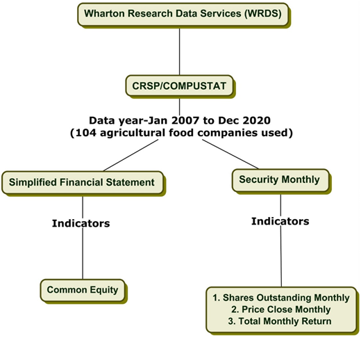
As shown in Figure 1, the data from the Simplified Financial Statement Extract and Security Monthly were obtained from the Center for Research in Security Prices (CRSP) and Compustat databases via WRDS. For each of the 104 companies, common equity data were sourced from the simplified financial statement extract. For the security monthly category, data collected included common equity, monthly shares outstanding, monthly closing price, and total monthly return indicators. Additionally, monthly treasury bill data, used as a proxy for the risk-free rate, were extracted from the FF3FM portfolios and factors vendors within the WRDS platform.

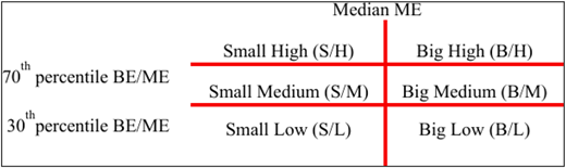
Following the methodology of Fama and French (1992, 1993, 1995, 1996), all agricultural food companies were grouped into six portfolios annually. The classification process began by ranking all the companies into two portfolios based on size, and then subdividing each size portfolio into three portfolios based on value. Specifically, companies were first divided into two size portfolios, including Small (S) and Big (B) portfolios, using the median market equity (ME) value of all the Agricultural food companies for that year as the threshold. Companies with ME values below the median were assigned to the S portfolio, while those above the median ME values were placed in the B portfolio. A company's annual ME was calculated by multiplying its shares outstanding monthly by the price close monthly data at the end of each year (a):

Next, companies within each size portfolio (S and B) were ranked annually based on their book-to-market equity (BE/ME) ratios for that year. Following Fama and French (1992), lagged BE/ME values were used, as book equity figures from financial statements are typically available only at the end of each calendar year. Using lagged value accounts for the delayed recognition of unexpected gains or losses, which are gradually reflected in book equity over time (Beaver and Ryan, 2000). To construct value-based portfolios, two cut-off points were applied: the 30th and 70th percentiles of the BE/ME ratios. Companies in the bottom 30th percentile were assigned to the Low (L) portfolio, those between the middle 30th and 70th percentiles to the Medium (M) portfolio, and those above the 70th percentile to the High (H) portfolio.

This ranking process yielded six distinct portfolios, categorized by both size and value, as illustrated in Figure 2. By intersecting the two size portfolios with three value portfolios, six portfolios were constructed for each year: Small ME and Low BE/ME (S/L), Small ME and Medium BE/ME (S/M), Small ME and High BE/ME (S/H), Big ME and Low BE/ME (B/L), Big ME and Medium BE/ME (B/M), and Big ME and High BE/ME (B/H).

This section provides a detailed description of the variables used in the analysis and outlines the application of the CAPM and FF3FM to assess portfolio returns. The analysis covers the period from January 2007 to December 2020, comprising 168 monthly observations (t) across six portfolios.

The dependent variable in both CAPM and FF3FM models is the excess return (⁠$Rit−Rft$ ) for each portfolio, which is formed based on the size and value of the companies. Excess returns represent the difference between the portfolio's actual returns (⁠$Rit$⁠) and the risk-free rate (⁠$Rft)$ at time t. This measure assesses a portfolio's performance relative to a risk-free benchmark, capturing the additional return earned for taking on market-related risks. It also provides a standardized basis for comparing returns across portfolios by isolating performance attributable to underlying risk factors.

Independent Variables include Market Risk Premium $(Rmt−Rft)$⁠, which is used in both the CAPM and FF3FM models. In addition, the FF3FM model incorporates two additional factors: Small Minus Big (⁠$SMBt$⁠), representing the size premium, and High Minus Low (⁠$HMLt$⁠), representing the value premium. Market Risk Premium $(Rmt−Rft)$ represents the difference between the market return (⁠$Rmt$⁠) and the risk-free rate (⁠$Rft$⁠) at time t. The market portfolio used in this study is based on a broad market index, providing a benchmark for comparing the performance of agricultural food company portfolios with the overall equity market. It reflects the additional return expected from a portfolio as compensation for its exposure to systematic risk.

Small Minus Big (⁠$SMBt$⁠) is the size premium. Based on long-term observations, smaller companies tend to outperform larger ones. $SMBt$ is calculated as the difference between the average monthly returns of the three small stock portfolios (⁠$RS/L,t,RS/M,t,RS/H,t$⁠) and the average monthly returns of the three big stock portfolios $(RBL,t,RBM,t,RB/H,t$⁠) as:

High Minus Low (⁠$HMLt$⁠) captures the value effect, reflecting the tendency of value companies, those with high BE/ME ratios, to outperform growth companies with low BE/ME ratios over time. $HMLt$ is calculated as the difference in average monthly returns between high book-to-market portfolios (⁠$RS/H,t,RB/H,t)$ and low book-to-market portfolios $(RSL,t,RB/L,t)$⁠, expressed as:

The SMB and HML factors are constructed using differences in average portfolio returns, following the standard methodology of Fama and French (1993). Although this construction is based on simple averaging of returns, it is designed to isolate systematic differences associated with firm size and book-to-market characteristics. The purpose of these factors is not to directly measure risk at the construction stage, but to create portfolios that proxy for underlying risk exposures. The relationship between these factors and risk is captured in the regression framework, where the estimated coefficients reflect the sensitivity of portfolio returns to these systematic risk components (Fama and French (1992). Therefore, the averaging approach is consistent with established asset pricing methodology and allows for the identification of size and value effects through their contribution to explaining excess returns.

The CAPM assumes that the market risk premium is the sole factor driving systematic risk in portfolio returns. By regressing excess returns on the market risk premium, the CAPM quantifies a portfolio's exposure to market risk. As a result, CAPM serves as a fundamental benchmark model for evaluating stock returns and guiding investment decisions.

The volatility was analyzed by a regression model:

Where, $αi$ represents the intercept, capturing the portion of returns not explained by the market risk premium. It reflects the average return attributable to factors not included in the model. $βi$ known as the market beta, measures the sensitivity of the portfolio's returns to movements in the overall market. A beta value greater than 1 implies that the portfolio is more volatile than the overall market, while a beta value less than 1 suggests lower volatility. $εi$ represents the error term accounting for unexplained variations and capturing random noise in portfolio returns.

The FF3FM model extends the CAPM by incorporating two additional factors: size and value. By including these factors, the FF3FM captures the observed tendency of small-cap stocks and high book-to-market stocks to outperform the broader market.

The regression equation is as follows:

Where $si$ is the sensitivity of portfolio i to the size factor (⁠$SMBt)$ and $hi$ is the sensitivity to the value factor (⁠$HMLt$⁠), respectively. A significant $si$ indicates that the portfolio has exposure to small-cap stocks, whereas a significant $hi$ reflects sensitivity to value stocks.

Time trends, seasonality, autocorrelation, and heteroscedasticity were checked for the time series regression (Bakar and Rosbi, 2019). The time variable was not significant across any of the six portfolios. To examine seasonality in stock returns, we created monthly dummy variables; however, we found no significant seasonal effects across all six portfolios.

Heteroscedasticity was assessed using the Breusch-Pagan and Cook-Weisberg test. In the CAPM regression, heteroscedasticity was detected in S/H and B/L portfolios and addressed by using robust standard errors. Similarly, in the FF3FM regressions, heteroscedasticity was identified in S/H and B/H portfolios and was also corrected with robust standard errors. Finally, the Durbin-Watson test was conducted to check for autocorrelation, and no evidence of autocorrelation was found in any of the portfolios.

Table 1 presents descriptive statistics for the period from January 2007 to December 2020, based on 168 monthly observations, highlighting variations in excess returns across six portfolios. The highest average return, 1.63%, is observed in the S/H portfolio, significantly outperforming the other portfolios. Apart from the S/H portfolio, larger portfolios generally exhibit higher average returns than smaller ones. This discrepancy can largely be attributed to the significant economic shocks of 2008 and 2020. The standard deviation indicates greater volatility among smaller companies, which typically face constraints in financial flexibility and resources. This observation supports the presence of a size effect in the stocks of agricultural food companies. Within both small and big portfolio groups, those with high BE/ME ratios (value portfolios) yield higher average returns: 1.62% for the S/H portfolio and 1.23% for the B/H portfolio. This trend demonstrates that high-value companies tend to generate higher average returns in the long term. These results suggest a value effect in agricultural food companies, whereby firms with higher BE/ME ratios are riskier but more profitable (Farooq and Morelli, 2015; Morelli, 2012). While these descriptive patterns are consistent with well-documented size and value effects in the broader equity market (Fama and French, 1993), it is important to consider whether they reflect characteristics specific to agricultural food companies. To provide context, the observed returns and volatility patterns in the agricultural food portfolios can be compared to those of the broader market. Although agricultural food companies exhibit similar factor-related behavior, their performance is influenced by sector-specific conditions, including commodity price cycles, climate-related risks, and policy interventions. These factors may contribute to differences in return dynamics relative to the overall market and may also help explain why agricultural food stocks are not always viewed as attractive investment options despite periods of favorable performance. Additionally, the average excess market return and HML factor show positive average returns, indicating that premiums exist to compensate for risk. Conversely, the SMB factor has a negative mean value, suggesting potential investment losses (Achola and Muriu, 2016; Eraslan, 2013; Pojanavatee, 2020). This negative size effect (SMB) may be attributed to the impact of economic recessions.

Table 2 examines the relationships among the six portfolios and key market indicators, revealing significant correlations. In particular, the market excess return is strongly correlated with all portfolios, with coefficients ranging from 0.83 to 0.92. The SMB factor displayed a positive association with smaller portfolios, indicating the presence of a size effect. Also, the HML factor is highly correlated with high BE/ME portfolios, suggesting a value effect. These results align with previous findings by Fama and French (2012) and Eraslan (2013), reinforcing the influence of size and value factors on the performance of agricultural food company stocks.

The CAPM regression results are presented in Table 3. The intercept in the CAPM represents the portion of portfolio returns not explained by market risk and can be interpreted as abnormal returns. Statistically significant intercepts indicate that the model does not fully capture the variation in returns and may reflect omitted risk factors or model misspecification (Fama and French, 1993). In this study, several portfolios exhibit significant intercepts, suggesting that the CAPM does not adequately explain excess returns for agricultural food companies. Although the adjusted R-squared values are relatively high, this is common in time-series regressions of portfolio returns on the market factor and does not, by itself, imply strong model performance.

Regarding beta values in the CAPM, our results are consistent with those of Pettengill et al. (1995), which show a significant positive relationship between portfolio returns and market excess returns. Four portfolios have beta values greater than one, indicating a significant positive relationship with the market excess returns. This implies that these portfolio returns are more volatile than the market returns. The highest beta value is observed in the S/H portfolio at 1.20, while the lowest is in the B/L portfolio at 0.69.

On average, the small portfolios (S/L, S/M, S/H) exhibit a higher beta, with an average of 1.15, compared to those of the big portfolios (B/L, B/M, B/H), with an average of 0.85. This indicates that smaller stocks are more sensitive to market movements and exhibit higher systematic risk. However, differences in beta alone do not explain the size and value effects, as these premia are defined by differences in average returns that are not captured by market risk. This limitation highlights the need for multifactor models to better explain the variation in returns (Schwert, 2002). In terms of the value effect, high portfolios (B/L, B/M, B/H) exhibit a higher average beta value of 1.13 compared to those of low portfolios, with an average beta value of 0.88, indicating that high-value stocks are more volatile than low-value stocks. This is consistent with the observation that value stocks tend to yield higher returns in the long run; however, these return differences are not fully explained by beta, reinforcing the importance of additional risk factors.

As shown in Table 4, the FF3FM yields statistically significant intercepts for several portfolios, indicating that the model does not fully capture the variation in excess returns. While the R-squared values are higher than those of the CAPM, high R-squared values are common in time-series regressions and do not, by themselves, validate the model. In this context, the behavior of the intercepts is more informative, as statistically significant intercepts suggest the presence of omitted risk factors or model misspecification (Fama and French, 1993). The coefficients on the SMB and HML factors are generally consistent in sign and significance across portfolios, reflecting differences in exposure to size and value factors. However, coefficient magnitudes alone do not establish the existence of return premia, as these premia are defined by differences in average returns rather than by factor loadings. Overall, while the FF3FM improves the explanatory power relative to the CAPM, the results indicate that it does not fully explain excess returns for agricultural food companies.

The beta coefficients are significant across all portfolios for the FF3FM, affirming the model's robustness. Our results align with those of Trimech et al. (2009), particularly in terms of the size effect. The SMB coefficient $si$ is significant in all six portfolios, reflecting the model's ability to capture the differential performance of small versus large firms. As in Bundoo (2008), the SMB coefficient is positive for all the small portfolios and negative for all the big portfolios. These patterns support Fama and French (1993) argument that opposite signs for the SMB coefficient across size categories between small and big portfolios reflect higher returns for small-cap portfolios relative to those for big firms.

The value effect, captured by the HML coefficient $hi$⁠, is significant in five of the six portfolios, with the exception of the S/M portfolio. This result aligns with Connor and Sehgal (2001). A closer examination of the HML slopes within each size portfolio shows that the slopes increase from low to high portfolios. The slopes of high portfolios are greater than low portfolios, which underscores the prominence of the value effect in agricultural and food companies during our study period (Fama and French, 1995; Penman, 1991).

Overall, the results provide strong evidence for the presence of both size and value effects, reinforcing the importance of including these factors in explaining the excess stock returns (Fama and French, 1993, 1995, 1996).

Table 5 summarizes the incremental explanatory power of the size (SMB) and value (HML) factors when each is added separately to the CAPM across the six portfolios. To compare the relative impact of the size and value effects, we separately added the size effect (SMB) and value effect (HML) to the market risk premium $(Rmt−Rft)$ of CAPM across all six portfolios.

Among the small portfolios (S/L, S/M, S/H), the value effect, except for the S/M portfolio, had a more significant impact on the excess returns than the size effect. This is evidenced by a larger increase in R-squared value, when the HML component was added to the CAPM, compared to the increase from adding the SMB component to the CAPM. Specifically, for the S/L portfolios, the R-squared increases from 69% to 85% with the addition of HML, versus an increase to 74% with SMB. For the S/H portfolios, the R-squared increased from 73% to 87% upon adding the HML component, compared to 80% with the SMB component. In contrast, the HML component was statistically insignificant for the S/M portfolio. These results suggest that the value effect has greater explanatory power in small portfolios, suggesting that value increases the explanatory power of the model in explaining the excess returns of small portfolios.

In contrast, big stock portfolios (B/L, B/M, B/H) appear more influenced by the size effect. Adding the SMB component to the CAPM led to greater improvements in model fit than adding HML. Specifically, the R-squared increased from 71% to 84% for B/L, 80%–91% for B/M, and 82%–88% for B/H with the addition of the SMB component. These increases were consistently higher than those observed when the HML component was added. This pattern suggests that the size effect may play a more prominent role in explaining excess returns in large-cap agricultural and food company stocks.

Overall, the results highlight that while the value effect dominates in small portfolios, the size effect contributes more significantly to the performance of large portfolios, reinforcing the necessity of a multifactor approach to accurately explain excess returns.

To compare the performance of the two pricing models, we followed the approach of Bartholdy and Peare (2005) and Sattar (2017), focusing on the significance of the intercept (A) and the magnitude of R-squared values. The comparative results are reported in Table 6.

For the CAPM, the average R-squared across the six portfolios is 76.53%. Additionally, most portfolios exhibit statistically significant intercepts, suggesting that the single-factor model fails to fully capture the variations in excess return of the portfolios and that additional explanatory variables are needed.

In contrast, the FF3FM yields a higher average R-squared value of 91.02%, and fewer portfolios showing significant intercepts. This improvement highlights the model's enhanced explanatory power through the inclusion of the size (SMB) and value (HML) factors. The higher R-squared value signifies that the two factors added to the CAPM increased the explanatory power in explaining excess returns. On average, the R-squared increased by 14.49% over the CAPM. These results are consistent with Fama and French (1993), who emphasized that size and book-to-market ratio formed variables (SMB and HML) are essential in explaining excess returns.

The FF3FM yields higher average R-squared values compared to the CAPM, indicating an improved model fit when additional factors are included (Grauer and Janmaat, 2010; Tambosi Filho et al., 2009). However, R-squared alone is not a sufficient criterion for evaluating asset pricing models, as high values are common in time-series regressions. In this context, the behavior of the intercepts provides more meaningful evidence. Although the FF3FM reduces the number of statistically significant intercepts relative to the CAPM, some portfolios continue to exhibit significant alphas, suggesting that the model does not fully explain excess returns. Therefore, while the FF3FM represents an improvement over the CAPM in explaining the returns of agricultural food companies, its explanatory power should be interpreted as relative rather than complete.

This study provides new insights into the risk-return characteristics of publicly traded agricultural food companies in North America by comparing the performance of the Capital Asset Pricing Model (CAPM) and the Fama-French Three-Factor Model (FF3FM). Traditionally, stocks in the agricultural sector were considered primarily as diversification tools due to their historically lower beta values (Clark et al., 2012). However, this research, which spans the period from 2007 to 2020, reveals a shift in this perception for agricultural food company stocks: seven out of twelve portfolios exhibit beta values greater than one. This suggests that agricultural stock may be evolving from diversification instruments into potentially profitable investment ventures.

The findings underscore that market volatility, represented by beta in the CAPM, is not the sole determinant of variation in portfolio returns. While the findings provide insights into the role of size and value factors in explaining excess returns, their implications for investors should be interpreted with caution. Investment decisions in agricultural food companies are influenced not only by risk-return characteristics but also by structural features of the sector, including relatively limited growth opportunities compared to high-growth industries and greater exposure to firm-specific and sector-level risks. In addition, agricultural assets are not necessarily perceived as low-risk, as they are affected by factors such as commodity price volatility, climate variability, and policy uncertainty. Therefore, rather than suggesting clear investment advantages, the results of this study are more appropriately viewed as contributing to an improved understanding of how systematic and sector-specific risks are reflected in the returns of agricultural food companies. This provides a basis for more informed evaluation of the sector within diversified portfolios, rather than as a standalone investment strategy.

Although the FF3FM outperforms the CAPM in this study, some intercepts remain significant, suggesting that other factors may influence excess returns. While the FF3FM improves the explanatory power relative to the CAPM, some intercepts remain statistically significant, indicating that additional factors may be relevant in explaining excess returns. Recent developments in asset pricing literature have introduced extended models, such as the Fama–French five-factor model, as well as intertemporal and consumption-based CAPM frameworks, which incorporate additional sources of systematic risk. Future research could extend the analysis by incorporating these multifactor models to assess whether they offer improved explanatory power in this sector, which may provide further insights into the behavior of agricultural food company returns.

In addition, the study period includes two major episodes of market stress the 2008 global financial crisis and the first wave of the COVID-19 pandemic which may have influenced the estimated return and risk relationships. Although diagnostic tests were conducted to verify the validity of the regression models, crisis-specific analyses, such as the inclusion of crisis-period dummy variables, subperiod estimations, or sensitivity analyses excluding crisis years, were beyond the scope of the present study. Future research could incorporate these approaches to better isolate the effects of extreme market events on the risk-return dynamics of agricultural food companies.