
Producers with electricity-intensive production systems face large bills with uncertain electric rate inflation adding to financial risk. Solar panels can reduce this risk, but producers hesitate to invest given lengthy payback periods, unpredictable reimbursement policy for solar electricity generation and high financial leverage. We demonstrate a decision aid for optimizing financing terms subject to amount and timing of federal income tax credits (ITC) and utility-specific rate structures.
The decision aid serves as (1) a benchmark for bids from solar installers; (2) an interface to break electricity rate structures into variable rate components vs fixed access and demand charges and (3) a tool to optimize loan length and amounts across two loans to lessen borrowing capacity and cash flow concerns.
Compared to a single 10- or 20-year loan for solar panels, a 10-year note together with a second loan repaid using ITC over the course of 1–5 years resulted in superior net present value (NPV), lower break-even electricity cost and addressed cash flow and borrowing capacity concerns. A longer 20-year note further eased cash flow issues at the cost of less favorable financial leverage and NPV.
Separating cash flow implications of subsidized solar investments into two categories, one for ITC realization and the other for equipment, allows for better loan collateralization. Using a unique set of firm observations, we arrive at system size and rate structure generalizations for Arkansas and beyond.
1. Introduction
In the poultry industry, electric utility charges are a large component of operating costs, as lighting and ventilation are energy intensive. Since integrators typically own the birds and feed, contract growers remain responsible for heating fuel, manure management, labor and housing charges in addition to electric utility charges. To lessen the latter electric utility costs, producers have and continue to investigate solar panel systems. With current state and federal regulations in place, purchasing a solar system can be favorable for agricultural operations. Indeed, the Inflation Reduction Act passed in late 2022 extended the income tax credit provision for solar investment originally at 26% of investment to 30% for installations between 2023 and 2033. There is also a low-income county provision that enhances the income tax credit to 40% and a further 10% increment to the income tax credit for solar panels if they are manufactured in the United States of America. At the same time, the bonus depreciation provision is being phased out. The bonus depreciation provision, essentially a tax break on a tax break, allows depreciating half of the income tax credit or 15% of the solar system purchase in the year of installation in addition to depreciation of the net investment (solar system purchase cost – income tax credit) using the five-year modified accelerated depreciation schedule. Installations initiated in 2023 allow capture of 80% of bonus depreciation, whereas 2024 installations are limited to 60% of bonus depreciation. Further annual 20% reductions of bonus depreciation completely phase out this program by 2027 (U.S. Department of Energy, n.d.).
Additionally, the state of Arkansas currently requires utility companies in the state to participate in 1:1 net metering. Net metering allows for kilowatt-hours (kWh) provided by the solar panel system and supplied to the grid to offset kWh drawn from the grid by the customer. When the customer sends more kWh to the grid than was actually used, their variable kWh charge for that month is zero, and the customer can be credited for the extra electricity (University of Arkansas Division of Agriculture Cooperative Extension Service, n.d.). Arkansas’ net metering provisions also allow month-to-month rollover within the same calendar year of any credits generated by the producer. Arkansas’ 1:1 net metering and rollover provisions currently provide one of the most favorable investment conditions in the USA. From an electric utility provider perspective, the rule favors the producer or electric consumer, as the electric grid serves as the backup “battery” when the solar system does not generate sufficient electricity to cover producer demand (nights and cloudy and/or rainy days). As such, only access fees and demand charges remain as the incentive for utility companies to provide this backup service and grid maintenance, as they have lost margin on variable rate kWh sales. Arkansas’ net-metering rules are changing, with current provisions set to expire in September 2024. At that time, 1:1 net metering will be replaced by an avoided cost reimbursement program, under which producer-generated electricity will be compensated at a wholesale rate rather than at the current retail variable rate.
Previous research has shown that investing in a solar panel system can be beneficial, predominantly from a net present value (NPV) perspective (Bateman, 2022). Other research finds that solar system size and compensation from utility providers are greater factors when evaluating the profitability of a solar panel system compared to solar availability (Brothers et al., 2022). Overall profitability depends on system size, buyback rates and tax incentives. The focus of this study is on the impact of varying loan characteristics used to finance solar investment.
The objective of this study is to evaluate how both loan length and loan structure (i.e. number of loans and their maturity) impact cash flows with solar investment vs the status quo of not investing in solar panels by continuing to solely source electricity from utility providers. We hypothesize that time to realize the federal income tax credit along with the number and length(s) of loans will have a significant impact on profitability that translates to different break-even electricity costs, financial leverage and cash flows over the long useful life of this type of investment. More specifically, to finance the initial investment, we optimize the split between short-term financing (repaid with the realization of the tax credit) and longer-term financing (repaid using solar revenue) to compare and to mitigate negative cash flow and borrowing capacity limitations associated with a single long-term loan under the assumption that most poultry growers, already highly financially leveraged, are cash-strapped to make equity contributions toward equipment investments on their farm as described further below. Hence, investigating two loans of different maturity instead of one long-term loan for this long-term investment is an alternative that lenders would appreciate as (1) default risk can be split across different lenders and (2) because cash savings from this investment occur over two distinct, different periods. First, potentially large income tax savings (ITS) occur at the onset pending ability to realize income tax credits, and second, annual electricity cost savings are more or less distributed in equal annual increments except for scheduled inverter replacement events for the remainder of the 30-year useful life of this investment. With different interest rates for different loan terms, producers thus stand to gain by optimizing the loan proportions toward this investment across two loans to (1) save on interest expenses and (2) match the timing of cash flow needs for loan repayment with cost savings from electricity generation and also income tax credit realization. This type of lending arrangement is not the current status quo.
2. Background and methods
Background. Previous analysis showed agricultural firms that are able to realize the income tax credit in the first year of investment would have a large positive net cash flow in terms of ITS in year one but experience negative cash flows with solar in following years until debt was repaid. This relatively long period of negative cash flows represents a significant barrier to producer adoption of solar systems (currently an estimated <1% of over 6,000 poultry producers have invested in solar panels (U.S. EIA, 2024; Liang, 2024). To mitigate these fluctuations in cash flow relative to the status quo of receiving electricity solely from the utility provider, we investigated using 10- and 20-year long-term notes to be repaid from solar revenue generation in conjunction with a second loan, repaid with the realization of the income tax credit (either within a year or over a period of 5 years) to observe the impact of loan length and number of loans on NPV over the 30-year useful life of the solar panel investment. As such, using mathematical programming, the size of the first and second notes could be optimized (based on the expected size and length of time to fully realize the income tax credit) to minimize negative net cash flow impacts relative to remaining with the status quo of no solar panel investment. Further, we assume the producer would finance solar system investment net of Rural Energy for America Program (REAP) grants that can provide from 15 to 50% of the initial cost of a solar panel system (USDA Rural Development, n.d.). An estimated 14 poultry farms received REAP funding over the period of 2018–2022 in Arkansas per communication with REAP staff.
Since income tax credits have a 3-year carryback provision and a 20-year carry forward provision, most producers, especially those building new facilities, are not expected to realize all their income tax credit in the first year. As such, we model both a 1-year short-term note for those that can realize the entire income tax credit in year 1 to cover the time between installation cost and tax savings realized at the end of year 1 and a longer time period. To assess profitability, NPV for solar investment using either 10-year or 20-year long-term notes, coupled with a second 1-year or 5-year short-term note, repaid on realization of tax credits are compared to after-tax NPV of the status quo of purchasing electricity from the grid without investing in solar panels. The five-year period for income tax credit realization was chosen arbitrarily.
We also solve for the break-even cost of electricity using solar in comparison to the current variable electricity rate using 35 farm operations with different electricity rate structures and size of systems to determine impacts of system size and variable electricity rates that depend on how much utilities charge for access and demand charges. Finally, we conducted a sensitivity analysis using an avoided cost rate provided by Entergy Arkansas, Limited Liability Company (LLC) (ESL Rate Administration, n.d.) to assess whether lower electricity buyback rates would impact the optimal number of loans to take on and what loan period to choose to repay debt.
Critical investment factors. To determine the feasibility of investing in solar panel systems for poultry producers in particular, but also commercial electricity users with high monthly utility bills, the effect of utilizing two loans with varying loan length terms on NPV and cash flows could be modeled with modifications to the Poultry Solar Analysis (PSA) tool (Popp et al., 2024). The PSA tool utilizes a producer’s past 12-month history of monthly utility costs to determine: (1) system size (Figure 1a and b); (2) cash flow implications over the 30-year useful life of the solar panel systems (Figures 2 and 3) and (3) break-even price for electricity (e.g. Figure 2a). The intent of the tool is to allow a user to enter operation-specific details to obtain interactive investment analysis results with limited effort.
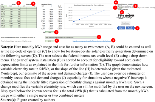
User interface for entering monthly electricity cost and quantity in the Poultry Solar Analysis (PSA) tool for sample Firm (A)
User interface for entering monthly electricity cost and quantity in the Poultry Solar Analysis (PSA) tool for sample Firm (A)
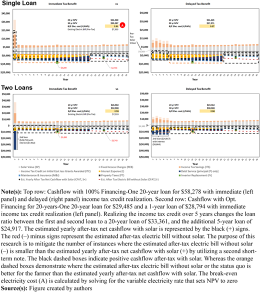
Impact of number of loans and time to realize income tax credit on cash flows, NPV, and break-even electricity cost using 20-year notes for solar panels for sample Firm A
Impact of number of loans and time to realize income tax credit on cash flows, NPV, and break-even electricity cost using 20-year notes for solar panels for sample Firm A
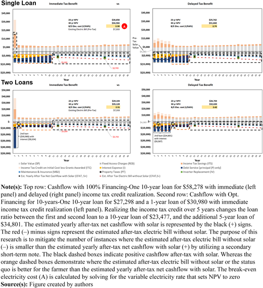
Impact of number of loans and time to realize income tax credit on cash flows, NPV and break-even electricity cost using 10-year notes for solar panels for sample Firm A
Impact of number of loans and time to realize income tax credit on cash flows, NPV and break-even electricity cost using 10-year notes for solar panels for sample Firm A
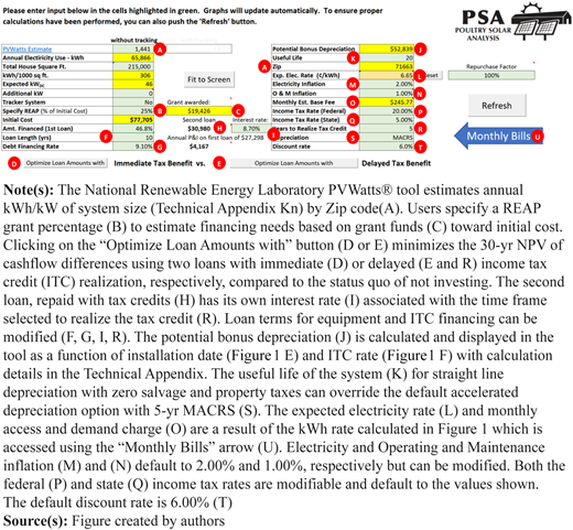
Given the need to estimate impacts of using two notes, alterations to the PSA tool required adding the ability to include a second loan (Figure 4h). Also needed was a Microsoft Visual Basic for Application macro that would solve for the optimal amount financed from a lender for each of the first and second notes (Figure 4d, e). The optimization involved minimizing negative net cash flow implications between the status quo of not investing and using 10- or 20-year financing to pay for an installation in light of expected ITS and utility bill reductions. With two loans, the second loan, repaid on realization of the tax credit, hinged on the expected time to realize the income tax credit (either within the first year (ITC1) or over the course of five years (ITCn)) (Figure 4r). The relative size of those two loans is expected to vary across the 35 firms analyzed as a function of system size (Figures 1k and 4a), time to realize the income tax credit (Figure 4r), loan terms (Figure 4f-i) and the variable electricity rate (Figure 1h) are expected to play a role that we aimed to quantify in terms of cash flow implications and NPV.
To estimate the impact of these decisions, we thus calculated NPV of solar investment as follows:
where IOi is the ith producer’s initial outlay subject to size of system or their past 12-months’ electricity use (Figure 1a, b and k), GAi is the REAP grant to assist with net investment (Figure 4b and c), CFATn,S+,ijk, described in greater detail below, represents the annual after-tax cash flow with the solar investment in year n that varies by the estimated ith producer’s variable and fixed electric utility charges, financing option j (choosing 1 or 2 loans) and loan term options, k, involving a choice of either 10- or 20-year. Loan lengths on the first note are secured by solar revenue and solar panel equipment and 1 or 5 years on the second note to be repaid using income tax credit savings. All cash flows are discounted using an annual opportunity cost of capital (d) of 6% (Figure 4t). Note that solar systems are expected to last 30 years.
Annual income tax credit savings are calculated as follows:
where (ITCn,ik) is the income tax credit in year n subject to the estimated initial investment less the grant awarded and the number of years it takes to realize the income tax credit (YITC,k). Further, pending county, the Office of Renewable Energy stipulates a 30% income tax credit rate (RITC) as a baseline with a provision to increase said rate to 40% in designated low-income counties or for native reservations. We used the 30% ITC rate and stipulated both a 1-year and 5-year time period for realizing the income tax credit in year 1 or evenly across years 1–5 (Figure 4r).
To allow the user of the PSA tool to examine the impact of different levels of grant funding on solar investment feasibility, the PSA tool was modified with a grant awarded section (Figure 4b and c). Grants awarded affect the calculation of net investment in the solar project that would then become the base for accelerated depreciation, income tax credit and loan repayment calculations. Agricultural producers and small rural businesses are eligible to apply for REAP grants. The program offers loan guarantees on loans up to 75% of total eligible project costs and grants up to 50% of total eligible project cost (USDA Rural Development, n.d.). For this research, a REAP grant of 25% was used, given feedback from solar installers and extension personnel that often assist with the paperwork for producers investing in solar equipment.
Also, net metering and meter aggregation were assumed. Meter aggregation allows solar panel systems to be sized to provide solar energy to the grid that is aggregated across meters for which the producer pays the utility company. For agricultural installations, utilities often provide several meters to (1) minimize demand charges; (2) allow for assessment of charges to smaller enterprise units that may be spatially distant from each other (e.g. irrigation vs machine shed vs poultry barn vs feed mill) and (3) minimize risk of electricity outage in the case only one enterprise is affected by a disturbance in a particular line segment.
In sum, after-tax cash flows are impacted by grants, loan guarantees, electricity rate structure and critical for this analysis, loan length terms and their associated principal and interest payments. Hence, generating a loan repayment structure that offers after-tax cash flows that are similar to or less expensive than those incurred without solar investment would be expected to lessen the hurdle to adoption of solar as a green alternative for electricity use. Using two loans and shorter repayment terms would also lessen lender and producer apprehension about investment in solar systems, as that investment and accompanying loans impact borrowing capacity for producers despite loan guarantees. Reduced borrowing capacity, through tying up equity in financing solar system investment, can be detrimental to poultry operations by impairing the grower’s ability to meet integrator demands for facility upgrades. In all types of agricultural operations, reduced borrowing capacity represents an increased risk for the operation. Ultimately, this hinders adoption of solar investment.
Mathematically, optimizing the after-tax cash flow implications of solar investment thus required calculation of CFATS+, the estimated yearly after-tax net cash flow with solar,
where the first line represents pre-tax solar value created (SP) that is subject to both annual electricity rate inflation (2%) and solar panel degradation (−0.5%) with the system sized to match annual utility needs currently met by the utility provider; income tax credit (ITC); federal and state ITS that are a function of depreciation, interest, maintenance and insurance (M&I); property taxes stemming from the investment in solar panels; the remaining fixed component of the electric bill (REB) and system upkeep with inverter replacement (IV) in years 12 and 24 (Figures 2 and 3). Note that these expenses vary by system size, lending options (number and duration on interest expenses only), bonus depreciation provisions given installation date and electricity rate structures that are separated into variable (including fuel surcharges) vs fixed (access and demand charges) rate components (Figure 1h and i). This delineation is important as electricity providers only reimburse variable rate components of the electricity bill and rate structures vary across the state’s 32 electricity providers. The second line of Eq. 3 represents financing costs where the proportion of initial cost net of awarded grant money is financed when: (1) one loan is pursued (AF) = 1 with either a 10- or 20-year payback provision; or (2) 0 ≤ AF ≤ 1 when two loans are pursued where the 1st loan leads to (P&I1) principal repayment and interest expenses given 10- or 20-year terms to finance the AFth fraction of financing needs with the remainder covered by the 2nd loan that leads to (P&I2) principal repayment and interest expense cash flows paid with ITS from the tax credit that can be realized over 1 or 5 years. Further details on these cash flow components are available in the technical appendix.
By comparison, CFATS-, is the estimated after-tax electric bill without solar.
where the after-tax estimated electrical bill without solar (CFATn,S-,i) for producer i is calculated using the estimated pre-tax electric bill without the system (EBn,i) that also inflates at the default 2% electricity cost inflation rate. We assume a state tax rate of 5%, and a federal tax rate of 20%. Note that a user can modify tax rates (Figure 4p and q). Also note that EB0,i is the producer’s current electricity bill with fixed and variable cost components as described further below.
Using the solver function in Excel®, we could then determine AF* as the optimal percentage of net investment in solar equipment financed by the first note by minimizing the NPV of differences between annual CFATS+ and CFATS- in years where CFATS + outflows were larger than CFATS- as follows:
where DCFijk are the present value of the sum of cash flow differences driven by financing options and income tax credit realization across 35 firms, four different loan options per firm based on (1) loan length (10-year or 20-year) and choosing 1 or 2 loans, with the same four loan options under either immediate or delayed income tax credit realization over the useful life of the installation. Note that AF* impacts CFATS+ (Eq. 3).
2.1 Data source
A 12-month record of electricity bills is required to assess annual kWh use and utility charges in the PSA tool. Such records were obtained during a solar lunch-and-learn extension presentation where poultry producers attended and volunteered their monthly electricity bills. Additionally, Delta Solar, an Arkansas-based company, offered bills from 26 agricultural installations (only identified by ZIP code) that included information regarding the number of meters, kWh per month and electricity bills paid over the most recent 12 months for installations that were in the planning phase or installed in 2021 and 2022. Using their ZIP codes (Figureas 1c and 4a), these 35 farm observations and the PVWatts® tool from the National Renewable Energy Laboratory (NREL, 2023) were used to estimate solar electricity generating potential, which varies by latitude, longitude and weather patterns, which in turn changes with the orientation of panels, their slope and/or whether the panels are fixed or track the sun’s movement. We utilized south-facing, fixed panels installed at a 20° tilt with weather patterns by ZIP code for all locations modeled (Figure 5). Further, Arkansas has 32 different electric utility providers, and each has different rate structures. By utilizing electrical bills from around the state, varying rate structures and locations could be analyzed with the PSA tool. We assumed these installations to offer a range of outcomes that potentially reflect outcomes for a range of investments. Assessing how representative this sample of utility bills is for agricultural operations in the state of Arkansas was deemed beyond the scope of this study.
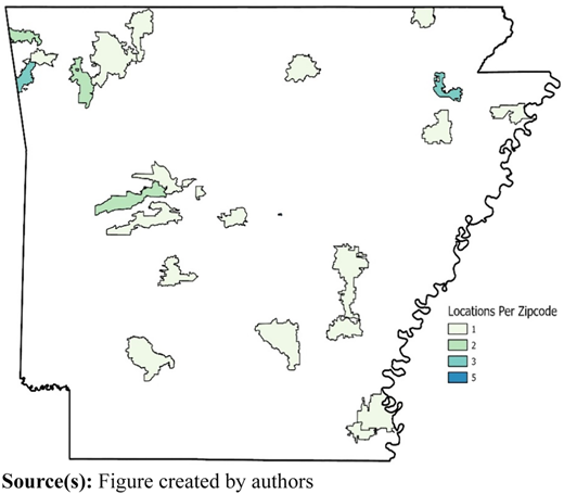
Locations in Arkansas from which the bills and installations used in this research were derived
Locations in Arkansas from which the bills and installations used in this research were derived
The total monthly electricity usage in kilowatt hours (kWh) for 12 months, demand charges for each month and ZIP code for each bill were used as input to the PSA tool (Figure 1a-c). Visually, data entry occurred as shown in Figure 1. Electricity usage and electricity charges were linearly regressed to determine the variable electricity rate (slope of the line – Figure 1h) with the intercept serving as the estimate of monthly access fees and demand charges (Figure 1i). Figure 6 shows a scenario where the estimated access fee was negative (Figure 6a). Since a negative access fee was counterintuitive, a $5.00 monthly fixed fee was arbitrarily assigned for five cases across the 35 farm situations and led to moderately higher annual electricity costs, as shown in Figure 6b.
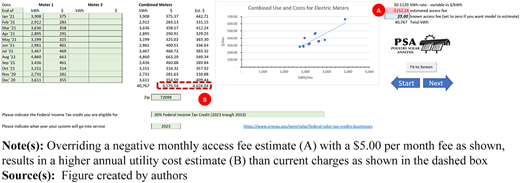
Example entry of modified monthly access fees and impact on overall annual utility charges for a sample Firm B
Example entry of modified monthly access fees and impact on overall annual utility charges for a sample Firm B
To compare 10-year and 20-year loan lengths, interest rates were needed. Farm Credit Service shared interest rates for 1-year fixed (8.45–8.95%), 10-year fixed (8.85–9.35%) and 20-year fixed (9.35–9.85%) notes (Figure 4g) in the spring of 2023. The mid-points of these ranges were used to calculate interest expenses on loans across all firms. A short-term rate of 8.7% (Figure 4i) served as the mid-point of rates used for the short-term notes for financing realization of income tax credits, whether 1 or 5 years in length. The technical appendix provides descriptions of calculations.
NPV and break-even electricity rates reflect a time value of money or capital recovery rate of 6% to reflect relatively low risk of investment in solar panels as a mature technology. Both investment NPV and NPV of cash flow differences between solar investment and the status quo use the 6% discount rate (Figure 4t).
2.2 Sensitivity analysis
In light of avoided cost reimbursement for solar generation coming into effect for solar installations deployed in late 2024, we conducted a sensitivity analysis across all 35 firms by replacing estimated variable electricity rates (Figure 4l) with an avoided cost rate. We used an avoided cost rate of 4.653 cents per kWh, which was the highest value of avoided energy costs of the annual average category provided in 2023 by Entergy Arkansas (ESL Rate Administration, n.d.). With month-to-month carryover provision changes, this avoided cost scenario is expected to proxy a worst-case scenario. Worst-case, in the sense that with net billing, utility providers would only value periodic production in excess of periodic use at the avoided cost rate. To model this, time-of-day use and solar electricity production as well as potential time-of-day electricity rate schedules and demand charges play a role in the sense that excess production is not carried forward or back over the course of a year to balance annual capacity to annual use. These considerations are deemed beyond the scope of this analysis. Instead, we use the existing setup of the decision aid under assumptions of net metering with carryover and replace the variable rate electricity with the avoided cost rate to analyze the impact on loan allocation (AF*) under a worst-case electricity rate reimbursement scenario.
3. Results and discussion
Using the PSA tool, we analyzed outcomes for all 35 firms using 1 or 2 loans, 2 loan lengths, 2 periods to realize income tax credits and 2 variable electricity rate estimates (16 scenarios per firm). We first describe relevant solar system characteristics for the 35 firms used for this analysis. Second, using a randomly chosen operation, we report on results for 20-year loan lengths in terms of time to realize the income tax credit and number of loans used. Third, 10-year loan length results are discussed in a similar vein. Fourth, we discuss the implications of loan length and time to realize the income tax credit on borrowing capacity for an operation near average in terms of investment amount. Fifth, we report on the electricity reimbursement rate sensitivity analysis including a firm with limited demand charges (Figure 6). Lastly, we report on system size effects.
3.1 Description of sample firms
Table 1 showcases the overall range in operation size across the 35 firms analyzed. The range in number of meters for all 35 operations varied from 1 to 38. The minimum current variable electricity rate in ¢/kWh was 5.70, with the maximum being 13.51. For the span in initial cost, the smallest investment was $24,000 and the largest totaled $2,494,000. The sizes of current annual electricity costs begin at $2,216 with the maximum being $274,604. As for the systems’ sizes in kWDC across all 35 operations, the smallest size equaled 14 kWDC and the largest operation required 1,848 kWDC where the latter sizes translate directly to the number of panels an operation uses to generate kWh.
Operation sample description with NPV, loan allocation and break-even (B/E) electricity cost results across 35 agricultural firms in Arkansas in 2023
| Min | Avg | Max | |
|---|---|---|---|
| # of Meters | 1 | 7.1 | 38 |
| Current variable electricity rate in ¢/kWh | 5.70 | 9.61 | 13.51 |
| Range in initial cost ($) in 000’s | 24 | 388 | 2,494 |
| Range of current annual electricity Cost ($) | 2,216 | 40,511 | 274,604 |
| Range of system size kWDC | 14 | 248 | 1,848 |
| Monthly access fee/demand charge est | 5 | 592 | 3,186 |
| With net-metering | |||
| NPV with immediate ITC capture (Opt. Fin.) ($) in 000’s | 20 | 307 | 2,249 |
| NPV with ITC captured over 5 years (Opt. Fin.) ($) in 000’s | 19 | 294 | 2,161 |
| Opt. Fin. (% of initial cost on long-term loan) - ITC 1 | 40% | 54% | 69% |
| Opt. Fin. (% of initial cost on long-term loan) - ITC n | 38% | 54% | 66% |
| B/E electricity rate immediate ITC capture | 2.20 | 2.35 | 2.63 |
| B/E electricity rate with ITC captured over 5 years | 2.48 | 2.66 | 2.89 |
| With avoided cost rate | |||
| Current variable electricity rate in ¢/kWh | 4.65 | 4.65 | 4.65 |
| NPV with immediate ITC capture (Opt. Fin.) ($) in 000’s | 6 | 99 | 684 |
| NPV with ITC captured over 5 years (Opt. Fin.) ($) in 000’s | 5 | 87 | 603 |
| Opt. Fin. (% of initial cost on long-term loan) - ITC 1 | 32% | 34% | 39% |
| Opt. Fin. (% of initial cost on long-term loan) - ITC n | 31% | 33% | 38% |
| B/E electricity rate immediate ITC capture | 2.17 | 2.32 | 2.61 |
| B/E electricity rate with ITC captured over 5 years | 2.44 | 2.61 | 2.85 |
Source(s): Table created by authors
3.2 Twenty-year note with immediate and delayed income tax credit realization
Figure 2 shows the cash flow for a randomly chosen Firm A using 100% financing with a single 20-year loan for $58,278 for a farm firm that had a starting annual electricity bill of $7,332.60 (Figure 5), which is below the average investment of the sample of operations investigated. While the initial estimated investment amounted to $77,705 for this 46 kWDC system, the 25% REAP grant lowered lending requirements by $19,426. In the scenario where a producer could take advantage of the income tax credit all in the first year, the estimated yearly after-tax net cash flow with solar (CFAT1,S+) is both positive and above the estimated after-tax electric bill without solar (CFAT1,S-) in the first year. For the next 19 years, the estimated CFATS+ is below the CFATS- as the producer repays the loan for the solar system, and as such, the solar investor has greater after-tax outlays with solar than without for 19 of the first 20 years. This is considered a large disincentive for most producers even when the installation is relatively small. Beyond year 20, the system yields large after-tax cash flow benefits (with the exception of year 24, when an inverter is replaced) as the loan on the equipment is fully repaid and the solar system continues to generate income. However, these distant future benefits are hypothesized to be insufficient for most producers to consider investment.
A similar issue arises when income tax credits are realized over a five-year period: years 6 through 20 show instances where cash flow is more negative than the status quo. Nonetheless, both of the investments, one with immediate and one with delayed realization of the ITC, led to a positive NPV over the 30-year investment horizon and thereby a break-even electricity cost of 2.91 ¢/kWh that is lower than the current electricity rate estimated at 6.65 ¢/kWh. Note that both inflate over time at the 2% inflation rate expectation.
3.3 Twenty-year note with a second note to match immediate and delayed income tax credit realization
The bottom left panel in Figure 2 compares the immediate tax benefit cash flows of a 20-year loan for $29,485 while also using a 1-year loan of $28,794. The latter note is repaid with the ITS and shows up as the larger principal and interest payment in year 1 in the bottom left panel of Figure 2. When realizing the tax benefit immediately, the CFATS+’s is only slightly below the CFATS-’s for the first year and the 12th year, when the inverter is replaced. In all other years, the solar system yields a positive after-tax cash flow in comparison to the status quo. From an annual cash flow perspective, this financing option is thus considered more enticing for producers. Also, the NPV is higher than with the single loan as interest savings are attainable with better cash flow matching.
Similar results occur with the delayed ITC scenario except that the optimal loan size for the first loan is now $33,361 and the second 5-year loan is $24,917.
3.4 Ten-year note with immediate and delayed income tax credit realization
Figure 3 demonstrates the cash flow for a single 10-year loan for $58,278 with 100% financing and the difference between the immediate tax benefit and delayed tax benefit. The cash flows with solar with ITC realized in year 1 are lower than without solar for 9 years compared to 5 years with the delayed ITC. However, despite the better cash flows with the delayed tax benefit, the immediate tax benefit has a larger 30-year NPV, as well as a lower break-even electricity cost.
3.5 Ten-year note with a second note to match immediate and delayed income tax credit realization
The bottom left panel in Figure 3 displays the immediate tax benefit cash flow for a 10-year loan equal to $27,298 and a second loan for 1 year of $30,980. With this scenario, the immediate ITC shows more occurrences of cash flows with solar being above cash flows without solar than the delayed ITC. Furthermore, the 30-year NPV is greater with the first-year tax benefit, and the break-even electricity cost is smaller. The delayed ITC scenario has a 10-year loan of $23,477 with a short-term note of $34,801. As mentioned previously, this scenario presents more instances of cash flows without solar being above cash flows with solar, a negative, from an annual after-tax cash flow perspective toward this financing method. Additionally, the break-even electricity cost is larger, and the 30-year NPV is smaller than with immediate ITC realization.
3.6 Impact on borrowing capacity
The 20-year and 10-year cash flow scenarios, along with the long-term nature of the investment, tie up significant borrowing capacity, as illustrated in Figure 7, showing the debt-to-asset ratio over the loan term using 30-year straight-line depreciation for asset valuation with zero salvage value for the solar system for an operation with average initial outlay (Firm C). This reduction in borrowing capacity is considered a disincentive for potential investors. With the two-loan scenarios, i.e. a 20-year plus short-term loan and the 10-year loan plus short term-loan, and immediate ITC realization, operators experience a high debt-to-asset ratio in the first year of investment, but it decreases significantly in the second year of investment. This situation looks more favorable to potential investors and lenders. The debt-to-asset ratio with a delayed ITC realization for the two-loan 20-year and 10-year options is lower compared to the financing with one loan but remains relatively high during the first five years with delayed ITC realization.
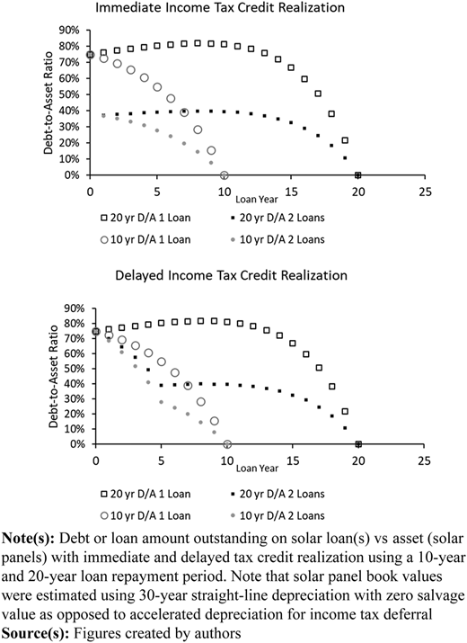
Impact of number of loans on borrowing capacity for the Firm C closest to average initial investment amount
Impact of number of loans on borrowing capacity for the Firm C closest to average initial investment amount
3.7 Optimal loan size range
The above discussion centered on Firm A that had a relatively small investment and Firm C with an average solar investment. Summarizing financing arrangement differences across all 35 firms, the largest percentage of initial cost with the long-term loan using an immediate income tax credit capture ranged from a high of 69% to a low of 40%. In the case of delayed income tax credit capture, the percentage of initial cost on a long-term loan ranged from a high of 66% to a low of 38%. Notably, Table 1 also shows the break-even electricity rates across all firms with both the immediate income tax credit and delayed income tax credit. Across both ITC realization scenarios, break-even electricity rates are smaller compared to the existing variable electricity rates experienced by the operations.
After data entry of monthly electric bill details in the PSA tool for each firm and analyzing all the data, a 10-year loan with a second shorter-term note resulted in superior NPV and the lowest B/E electricity cost. Additionally, the 20-year loan with a second note had the least amount of incidences of higher cash outflows with solar installations in comparison to the status quo. Table 2 presents a comparison across loan and income tax credit scenarios with respect to cash flow differences (Eq. 5) between solar investment and the status quo of remaining with the electrical grid. It summarizes the gap between CFATS + vs CFATS-, termed negative cash flow, as showcased in Figures 2 and 3 for a small installation, across all firms instead. Spreading income tax credit realization over more years reduces the incidence of negative cash flows, as does financing over a longer period, though with the tradeoff of reduced borrowing capacity (Figure 7).
Present value (PV) of cash flow differences in years when investing in solar vs the status quo led to higher cash outflows with investment than the status quo across 35 agricultural firms in Arkansas (2023), using net metering
| Min | Avg | Max | |
|---|---|---|---|
| 10-yr. 1 loan | |||
| Total PV of Neg Cash flow 1 yr | −$559,251 | −$103,363 | −$5,565 |
| Total PV of Neg Cash flow 5 yr | −$291,947 | −$53,749 | −$2,901 |
| 20-yr. 1 loan | |||
| Total PV of Neg Cash flow 1 yr | −$160,637 | −$38,495 | −$541 |
| Total PV of Neg Cashflow 5 yr | −$116,234 | −$28,606 | −$541 |
| 10-yr. 2 loans | |||
| Total PV of Neg Cash flow 1 yr | −$20,455 | −$2,823 | $0 |
| Total PV of Neg Cash flow 5 yr | −$54,110 | −$10,864 | $0 |
| 20-yr. 2 loans | |||
| Total PV of Neg Cash flow 1 yr | −$5,826 | −$1,156 | $0 |
| Total PV of Neg Cash flow 5 yr | −$12,203 | −$2,007 | $0 |
Source(s): Table created by authors
3.8 Avoided cost scenarios
The bottom section of Table 1 displays the results from conducting the sensitivity analysis with the avoided cost rate. With the lower rate, the NPV for both immediate and delayed income tax credit decreases compared to the net metering scenario, as expected. Interestingly, the optimal financing amounts for the long-term equipment notes also decline. The break-even electricity rate for both immediate and delayed ITC capture also decreases slightly compared to the net metering scenario. We attribute lower break-even prices with avoided cost to the use of more short-term financing using a second loan at lower short-term financing cost (8.7 vs 9.1% or 9.6%) as AF* are smaller given smaller negative cash flow implications beyond debt repayment with avoided cost than net metering. While this seems to suggest that avoided cost pricing is better from a break-even electricity cost perspective, the lower NPV is surely expected to lead to lower producer adoption.
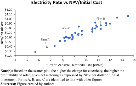
3.9 Economies of scale
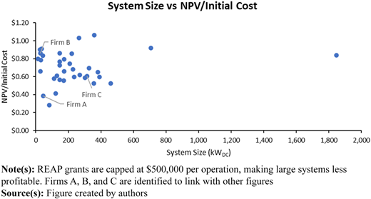
We were also interested in discovering the relationship between electricity rate and NPV in relation to initial cost (Figure 8). A larger number indicates greater profitability that should be a function of the utilities’ buyback rate. Given net metering, this relationship holds and suggests that lower avoided cost rate remuneration will lead to a substantial reduction in NPV. Additionally, in Figure 9, we plot the same profitability index (NPV in relation to initial cost) against system size. At the small end of the size spectrum, there is an upward trend given pecuniary economies associated with per-kW cost for panels detailed in the Technical Appendix. However, for larger operations, the REAP grant is capped at $500,000 per operation, reducing this size advantage.
4. Conclusion
The study presented in this paper evaluated how both loan length and number of loans affect cash flows with solar investment vs the status quo of not investing in solar panels and continuing to buy electricity from utility providers. The goal of using two loans was to mitigate negative cash flow implications between solar investment and the status quo by more closely matching loan repayment to the two different sources of returns to the system: utility savings and income tax credits. A sensitivity analysis was also conducted to determine the potential impact of avoided cost rates on solar panel investments. The results of the analysis suggest that employing two notes – one, finance the equipment and a second, repaid on the realization of tax credits – can (1) lessen cash flow stress associated with using a single loan (early after-tax cash flow improvement given ITS from the income tax credit provision and bonus depreciation followed by long periods of larger after-tax cash outlays in comparison to not investing in solar panels) and (2) better manage borrowing capacity limitations of a single loan as a large portion of the initial investment is paid off early with the second loan using cash flow gains from tax breaks generated early on. Employing two loans may thus increase the likelihood that a producer would invest in solar panels, as after-tax cash flows are consistently better with solar investment than without when loan terms are matched to two distinct sets of cost savings with different time horizons.
Lower NPVs were estimated when producers are reimbursed at an avoided cost rate that is substantially lower than current variable electricity rates some utility providers charge. Targeting larger firms because of pecuniary economies of size is not expected to offset these negative changes for producers. Nonetheless, the PSA tool offers users insights about how to finance this type of investment. An analysis of alternative interest rate differentials between short- and longer-term financing is left for further research, as are implications about electricity rate inflation expectations.
From a policy perspective, larger installations are more cost-effective from a pecuniary economies-of-size perspective that could be even greater if the REAP grant cap were removed. However, the chance of finding larger parcels of land that do not interfere with taking productive agricultural land for food, feed and fiber production out of production is greater with larger installations. Notably, small installations still offered positive NPV with a greater likelihood of not impacting food, feed and fiber production, as smaller unproductive parcels of land are easier to find than large ones. Finally, fewer larger installations may be prone to greater electricity interruptions in case of inclement weather disruptions (tornadoes, destructive hail and straight-line winds) than a larger number of smaller installations. The provision of loan guarantees should assist both small- and large-scale installations. Loan guarantees could stipulate setting up two loans as a requirement to better match cost savings to loan repayment needs.
Funding: This research was funded by a USDA ERS Collaborative Agreement. The findings and conclusions in this article are those of the authors and should not be construed to represent any official USDA or U.S. Government determination or policy. This research was supported, in part, by the U.S. Department of Agriculture, Economic Research Service.
References
Further reading
Technical appendix
Parameters for cost and revenue calculations per equations in the text
| Variable name | Description |
|---|---|
| For Equation 1: Net present value (NPV) as a function of system size and grantsmanship | |
| IOi | Initial outlay in the year of installation is dependent upon system size. The ith producer’s past 12-months’ electricity use determines annual kWh which is subsequently divided by the solar electricity production potential per kWDC where the latter is a measure of system size in a physical sense. For installations less the 200 kWDC in size the cost is $1,700/kWDC, for installations between 200 and 499 kWDC ($1,610/kWDC), 500–999 kWDC ($1,510/kWDC), 1–1.999 MWDC ($1,350/kWDC), 2–4.999 MWDC ($1,290/kWDC), 5–9.999 MWDC ($1,280/kWDC), 10–19.999 MWDC ($1,260/kWDC) and 20+ MWDC ($1,250/kWDC). These costs reflect estimates provided in 2022 by Delta Solar, an Arkansas based solar installer, for fixed panels. The cost estimates are similar to those available at the National Renewable Energy Lab (NREL). For installations greater than 500 kWDC, tracking technology can be used at an upcharge of 10% with an average productivity increase of 18%. Tracking technology is not evaluated in this analysis. Solar electricity production potential per kWDC were obtained using the PVWatts tool available at NREL. |
| GAi | The Rural Energy for America Program (REAP) offers producers grants of 15–50% of eligible project costs (IOi) with a maximum of $500,000 per operation. Funding for these grant applications varies. We use 25% in this analysis. |
| For Equation 2: Annual income tax credit (ITCn,ik) as a function of income tax credit rate and years to realize the credit | |
| RITC | The income tax credit rate is set to 30% per recent legislation for installations between 2023 and 2033. Low-income county, native reservation and/or U.S. manufacture of panels offers higher rates. More details are available at https://www.energy.gov/eere/solar/federal-solar-tax-credits-businesses |
| YITC,k | Number of years to realize income tax credit is set to either 1 or 5 years in this analysis. |
| For Equation 3: Cash flows after-tax with a solar system (CFATn,S+,ijk) are a function of solar electricity generation, ITC, depreciation, maintenance and insurance, property taxes, remaining electric bill, inverter replacement and repayment of loan(s) | |
| SPn,i | Pre-tax solar value in year n = Kn,i * ERn,i where Kn,i is the amount of kWh produced by the system which depends on system size for the ith producer in kWDC and the ZIP code-dependent amount of kWh produced per kWDC; and ERn,i is the ith producer’s variable electricity rate obtained from regressing their monthly electricity charges against their kWh use. The y-intercept of said regression serves as the estimate of monthly fixed access and demand charges (REBi) whereas the slope estimate is the variable electricity rate. We set the electricity inflation rate at 2% per year. Solar electricity generation (K) degrades at 0.5% per year |
| ITCn,ik | see explanation for Eq. 2 |
| For Equation 3 (cont’d) | |
| DEPik | Solar panel depreciation for tax purposes in year n (n = 1,2,3,4,5,6) derived using 5-yr Modified Accelerated Capital Recovery System (MACRS) rates (Yr 1 = 20%, Yr 2 = 32%, Yr 3 = 19.2%, Yr 4 = 11.52%, Yr 5 = 20% and Yr 6 = 5.6%). Although the income tax credit essentially lowers the purchase price of the system, the depreciable amount of the system allows for depreciation of half the income tax credit. With a 30% income tax credit, 85% of the purchase cost is eligible for depreciation. Further, pending year of installation, 80% of depreciation can be tax deductible in Yr 1 if installed in 2023, 60% with installation in 2024, 40% in 2025 and 20% in 2026 and is commonly referred to as bonus depreciation. The remainder of depreciation after bonus depreciation is spread over the six-year schedule if the producer is assumed to be able to realize income tax credits in the first year. With delayed income tax credit realization we depreciate using 5-yr MACRS adding half the income tax credit across the six-year schedule. The user has the option to modify 5-yr MACRS to straight line depreciation with zero salvage over a user-specified useful life. This latter option was not used in this analysis |
| M&In,i | Maintenance charges are set to $5.00 per kWDC with an additional $5.50 per kWDC for insurance based on personal communication with Dr. Brothers (2022). Both inflate at an estimated 1% per year using similar assumptions as those provided in the System Advisor Model (SAM) of NREL. Maintenance costs increase by 10% with tracking technology which was not modeled in this analysis |
| PTn,i | Property tax expenses in year n were based on a property tax rate of 0.75% of book value using straight line depreciation and a 20 yr useful life with zero salvage value and IOi as the initial cost of the Solar System |
| REBn,i | The y-intercept of the regression of monthly utility charges against kWh use serves as the estimate of monthly fixed access and demand charges that are multiplied by 12 months to calculate annual charges. If estimated REBi are negative, a $5/month charge was assumed with the variable electricity rate (ERi) modified to fit the linear regression through the modified y-intercept and average monthly charges and use. These charges inflate at 2% per year |
| IVn,i | Inverters are needed to convert direct current from solar panels to alternating current before grid connection. Inverter replacement occurs in years 12 and 24 over the life of the system. Inverter replacement costs $70 per kWDC in year 12 and $60 per kWDC in year 24 (Source: Personal communication with Dr. Brothers, Delta Solar and SAM tool provided by the National Renewable Energy Lab) |
| For Equation 3 (cont’d) | |
| ITSn,ijk | Depreciation, maintenance and insurance, property taxes, remaining utility charges, inverter replacement and interest charges on financing are all tax deductible. State income tax savings were calculated using a 5% state income tax rate. Federal income tax savings were calculated using a 20% federal income tax on the same cost items net of state income taxes. The PSA tool user can modify tax rates. Interest expenses vary for the ith producer based on number of loans, loan length and time to realize income tax credit |
| AFijk | Fraction of financing needs (IOi – GAi) secured by solar panels, solar generation and income tax credits is set to 1 or 100% if using one loan to repay over either 10 or 20 yrs. A second loan option is available to finance income tax credit realization over 1 or 5 yrs separate from the first loan now secured by solar panels and solar generation only. Financing options and realization of income tax credits and hence impacts timing of principal payments and interest cost |
| P&I1,n,ijk | Principal and interest on the first (equipment) loan |
| P&I2,n,ijk | Principal and interest on the second (ITC) loan |
| For Equation 4: Cash flows after-tax without a solar system (CFATn,S-,ijk) is a function of electricity use, electricity inflation and state and federal income tax rates | |
| EBn,i | Annual electrical bills as provided by producer i inflate at 2% per year. Since utility charges are income tax deductible, we calculate after-tax electricity charges as shown in the text. Note that electricity use is not modeled to change over the 30 yr useful life of the system which is appropriate as long as electricity use does not decline over time |
Source(s): Table created by authors
