


The paper aims to shed light on the effects of inflation on gold price and exchange rate in Vietnam by using time-varying cointegration.
Using cointegration techniques with fixed coefficient and time-varying coefficient, the study exams the impacts of inflation in models and compares the results through coefficient estimates.
A significant inflation impacts are found with the time-varying cointegration but not with the fixed coefficient cointegration models. Moreover, monetary policy affects exchange rate not only directly via its instruments as money supply and interest rate but indirectly via inflation. Also, interest rate is one of the determinants of gold price.
To the best of our knowledge, this paper is the first to use time-varying cointegration to analyze the impact of inflation on the gold price and exchange rate in Vietnam. Gold price and exchange rate fluctuations are always the essential and striking issues, which have been emphasized by economists and policymakers. In macroeconometric researches, cointegration models are often used to analyze the long-term relations between variables. Attentionally, applied models show a limitation when estimating coefficients are fixed. This characteristic might not really match with the data properties and the variation of the economy. Currently, time-varying cointegration models are emerging method to solve the above issue.
1. Introduction
Time-varying cointegration has been concerned as an emerging method for investigating a long-run relationship in replacing fixed coefficient cointegration. The model with fixed coefficients expresses some inconsistencies of data characteristics and the actual issues happening in the economy. In macroeconomics, researchers have applied this method to solve the model and suggest recommendations and policy implications to adjust the amount of money supply to be equal to money demand for well-controlling inflation and achieving other goals of the monetary policy. However, the estimated coefficients are assumed to be constant over the investigation period. As a result, this approach can lead to inconsistent estimates in quantitative models, ineffective expected results of policy implications. Therefore, time-varying cointegration is documented better than fixed coefficient cointegration (Bierens and Martins, 2010; Chang et al., 2015; Koop et al., 2011; Zuo and Park, 2011).
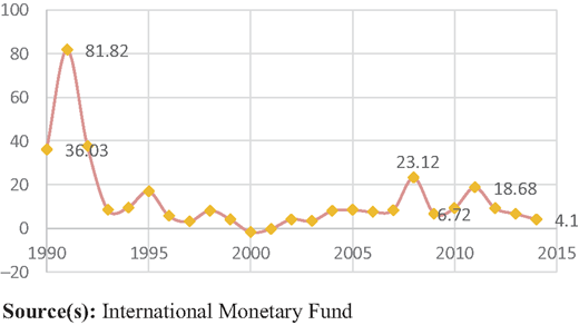
Whether the above approach can be applied in researching the impacts of inflation on gold price and exchange rate depends on nature and circumstances of the economy. In a developing country like Vietnam, the key factors of macroeconomics and economic policy have changed dramatically in most recent decades, especially during the financial crisis in 2008. After the economic reform during the 1990s, the inflation rate was still unstable (Figure 1). Specifically, the inflation rate in 1991 increased more than two times than the previous year and then fell down sharply in the following years. During the research time span, it tends to keep under 20%. However, the inflation rate reached the peak at approximately 23% in 2008 at the beginning of the world financial crisis. If inflation was not controlled well at a low level, it would harm the economy, leading to falling output, business bankruptcies, losing confidence in the domestic currency. Consequently, people tend to consider other safer assets, especially increase holding gold and foreign currency. Among this, gold price and exchange rate are two of the striking issues that economists and policymakers have been concentrating due to facing some difficulties in analyzing techniques.
Currently, the empirical studies relating to time series data for the case of Vietnam have inherited the fixed coefficient cointegration approach to analyzing the long-run relationship between the variables. First, for exchange rate, the validity of the prediction does not reach actual tendency due to a limitation of some statistical methods and extend the length of sampling (Park and Park, 2013). The elasticities of these factors were assumed not to vary over the period (Mark, 1995). Thus, inconsistent results may lead to the failure of exchange rate prediction model when using fixed coefficient. According to Beckmann et al. (2011) and Park and Park (2013), if time-varying cointegration is applied in the exchange rate prediction model, the result will be better in the analysis. Second, keeping gold is one of possible considering to hedge against inflation, especially in developing countries including Vietnam (Batten et al., 2014; Truong et al., 2017). This matter is not well investigated for the case of Vietnam. Whereas, some empirical researches, applying time-varying cointegration, have found evidence for the relationship between gold and inflation with sensitivity to interest rate changes (Batten et al., 2014; Lucey et al., 2016). In addition, gold has a role to protect against the growth of money supply in American economy (Lucey et al., 2016). In addition, using time-varying cointegration for detecting relationships among inflation, exchange rates, money demand function, the price of gasoline, rice price has brought the robust results in many countries all over the world (Bierens and Martins, 2010; Granger and Lee, 1991; Park and Hahn, 1999).
In regards to methodologies in the previous studies, the fixed cointegration methods such as VAR, VEC, ARDL were used to examine gold price and exchange rate (Arfaoui and Ben Rejeb, 2017; Batten et al., 2014; Seyyedi, 2017). However, it has been argued that financial liberalization, changes in monetary policy and lack of time series data can cause hardly estimates and unpredictable prediction in the relationships between macroeconomic variables. This implication motivates to extend the existing model estimation to the time-varying approach (Park and Zhao, 2010; Zuo and Park, 2011).
To the best of our knowledge, this paper is the first to use time-varying cointegration to analyze the impact of inflation on the gold price and exchange rate in Vietnam. While exchange rate can be recognized as one of the final targets of the monetary policy, gold price is emphasized for the government and investors. As this research can fill this gap in macroeconomic literature, the impacts of inflation on exchange rate and gold price can be unlocked by resolving the limitation of fixed coefficient cointegration. Accordingly, the model estimation output can interpret the role of inflation when performing time-varying Canonical cointegration, which is not detected by fixed coefficient cointegration. In addition, income and monetary policy proxies confirmed the consistency of two cointegration regressions.
The paper is organized as follows. Section 1 highlights briefly the current issue of cointegration with fixed coefficient as well as the motivation of time-varying cointegration in the analysis of inflation impact on gold price and exchange rate in Vietnam. Section 2 presents the methodology in time-varying cointegration approach and time-varying Canonical cointegration for the multivariate variable. From this, the model specifications and data source are described in Vietnam case study. The result of empirical study is analyzed in section 3. The final section gives conclusion for some remarkable implication.
2. Methodology and data
2.1 A cointegration regression: time-varying approach
According to Chang et al. (2015), Koop and Korobilis (2013), Kumar et al. (2012), Park and Park (2013), Park and Zhao (2010) and Zuo and Park (2011), the cointegration approach is expanded by allowing the coefficient in a dynamic model with time-varying. The estimated time-varying parameter (TVP) has two components including a “permanent component” as the traditional cointegration coefficient and a “temporary component”. The temporary component was estimated by using a different approach like ARIMA forecasting model. The TVP cointegration is described by equation (1), where qt is stationary I(0). There are two notices. First, At is a deterministic component such as constant and other components such as cosλt, tδ, some parametric function of time or a seasonal sequence Second, với Dt denoted an observation variable. Equation (1) can be rewritten as equation (2).
where with f(t) is a deterministic function of t or an observed variable Dt. The procedures of time-varying cointegration are summarized in four steps. Especially in the second step, coefficient At is assumed with very slowly time-varying change in a random walk model. The process of residual pt is assumed based on autoregression AR(1) and can be extended easily to other ARIMA models (p, q).
Step 1: Check stationary xt and yt whether exist I(1) (general TVP-I(1)) or not.
Step 2: Perform time-varying cointegration to estimate coefficient.
Step 3: Select the best forecasts model among cointegration with fix coefficient.
Step 4: Perform t statistic in time-varying cointegration.
2.2 Time-varying Canonical cointegration for multivariate variables
Following Granger and Lee (1991), a time-varying model with an elasticity αt changing over the time is given by equation (3), denoting as a function of Fourier Flexible Form (FFF). Particularly, it is performed by equation (4).
where is estimated by an FFF as p and q increase. Let denote and , the model presents the coefficient as or with . To put it in this, this non-linear function can be estimated by a linear function with a regress and . The time-varying cointegration (TVC) is shown by equation (5).
where is a matrix of regressors and is a matrix of coefficients. The error term is merged from the original disequilibrium error and an approximation error from fixing p and q. When p = q = 0, this is a special TVC model with which is performed as fixed coefficient cointegration regression.
The model assumes that vector cointegration exists. Where matrix xd contains the independent variables which do not include the variable with the elasticity of time-varying coefficient such as xt. Defining , the model supposes that there is no inconsistency of wt so that . Where B = BM(Ω) is the Brownian dynamic component with variance Ω. Where . Denoting and , the model uses long-run variance . Where ω11 is a variance of (ut) and Ω22 is a variance of (Δxt, Δpt)'. The matrix of Δ and Σ is separated appropriately.
The CCR model can be estimated following two steps. First, equation (6) is performed by ordinary least square (OLS) and is constructed with a consistent variance. Consistent long-run variance estimators are acceptable. By using to estimate appropriately, equation (7) of the model shows the CCR construction model with a vector .
Equation (7) is reduced by equation (8) error term with . The CCR model can be estimated by OLS but standard errors of these variables are estimated from the variance . Where is consistent by using the variance of the previous regression.
2.3 Model specification
The quantitative method is used as follows. The first step is unit root test to check the stationary characteristic of all variables. The second step is Johansen's cointegration test to confirm the long-run relationship. In the third step, model estimation uses different techniques including fixed coefficient cointegration and time-varying cointegration. The long-run variance of the CCR model is mentioned to remedy correlation and endogenous phenomenon (Wang and Wu, 2012). A time-varying cointegration is enhanced in the CCR model that performs the time-varying parameter estimates (Chang et al., 2015; Lucey et al., 2016; Park and Park, 2013). In order to analyze the impact of inflation on the gold price and exchange rate, the paper considers the previous studies for model 1 (Chang et al., 2015; Park and Hahn, 1999) and model 2 (Batten et al., 2014; Lucey et al., 2016). The monetary policy is added as group control variables through real deposit interest rate () and broad money supply M2. It can be presented as the monetary policy tools. Moreover, income is selected by domestic industrial value (). Consumer price index () represents inflation which has a time-varying elasticity . The dependent variables of the two models are real domestic gold price () and real effective exchange rate . As a result, two models will be proposed in equations (9) and (10).
2.4 Data source
This study uses monthly time series data from 2003 Dec to 2016 Feb (see Table 1). In order to standardize and adjust the data, natural logarithm form will be applied for , , . These variables are depersonalized using seasonal dummies. , and are presented in percentage.
Data source description
| Variables | Description variables | Data source |
|---|---|---|
| Real gold price | General Statistics Office in Vietnam, doij.com | |
| Real effective exchange rate | Darvas (2012) and update to period research | |
| Consumer price index | International Monetary Fund (IMF) | |
| Real industrial production value | General Statistics Office in Vietnam | |
| Real deposits interest rate | International Monetary Fund (IMF) | |
| Real broad money supply M2 | International Monetary Fund (IMF) |
Note(s): In data source, the real variables are converted from given nominal variables
3. Empirical result
3.1 Full sample unit root and cointegration test
Table 2 summarizes the outcomes of ADF and ADF with breakpoint structure unit root tests on the level at first differences of the variables. The null hypothesis cannot reject that all the variables are unit root at zero difference, except broad money supply. However, all of them are stationary with 1% significance level when conducted the first difference. The result suggests that all variables are I(1), which supports the use of the cointegration approach. Next, the paper exams the existence of long-run equilibrium. The result of Johansen test is tabulated in Table 3. The critical value (87.31) exceeds the trace test (79.38) at 5% significance level. It implies to reject the null hypothesis. Alternatively, the maximum rank indicates one cointegration equation at 1% significance level. As these conditions are satisfied, the next step for regressions will be conducted.
The result of unit root test
| Variables | ADF test | ADF with breakpoint structure test | ||||
|---|---|---|---|---|---|---|
| Level | 1st difference | Level | Break date | 1st difference | Break date | |
| −2.236 | −8.885*1 | −5.178*5 | 2006m12 | −5.288*5 | 2007m6 | |
| −0.974 | −8.602*1 | −3.645 | 2013m1 | −10.928*1 | 2006m6 | |
| −2.003 | −14.343*1 | −5.57 | 2012m2 | −14.746*1 | 2012m2 | |
| −2.391 | −9.273*1 | −3.735 | 2010m7 | −9.907*1 | 2008m12 | |
| −0.0281 | −7.704*1 | −2.791 | 2007m11 | −8.990*1 | 2009m2 | |
| −1.706 | −4.947*1 | −3.650 | 2010m11 | −6.619*1 | 2010m9 | |
Note(s): (*1), (*5), (*10) denote the significance at the 1%, 5%, and 10% levels of Zt value; 1% = −4.025 (*1), 5% = −3.445 (*5), 10% = −3.145 (*10) (ADF test); 1% = −5.57 (*1), 5% = −5.08 (*5), 10% = −4.82 (*10) (ADF test with breakpoint structure)
3.2 The result of fixed coefficient and time-varying coefficient cointegration
As being contrary to the expectation, there is no existence of inflation impact on gold price (model 1) and exchange rate (model 2) if fixed coefficient cointegration is used (Table 4). Basically, when inflation increases, gold is an important asset instead of holding money. For model 1, only income negatively affects gold price in a long-run relationship at the 1% significant level. In contrast, for model 2, income negatively influence exchange rate.
Fixed coefficient cointegration for gold price and exchange rate
| Coefficients | Gold prices | Exchange rates | ||
|---|---|---|---|---|
| Estimates | t-value | Estimates | t-value | |
| τ | 24.8509*1 | 3.0318 | 94.8905*1 | 32.5734 |
| β | −0.00377 | −0.6158 | −0.00153 | −0.6982 |
| γ | 0.17454 | 0.5397 | 0.03317 | 0.2881 |
| ξ | −0.4455*1 | −2.1478 | 0.1553*1 | 2.0969 |
| α | 0.00281 | 0.4848 | 0.00042 | 0.20348 |
| Long-run variances of the CCR errors | ||||
| ω2 | 0.10734 | 0.01442 | ||
Note(s): *1 denotes the significance at the 1% level of Zt value
However, when the study examines model 1 and model 2 using time-varying cointegration, the results are differently revealed in Table 5. The inflation variable has effects on both gold price and exchange rate respectively. Model 1 points out that the impact of inflation tends to decrease (λ3) and recover with an increasing trend (λ6) afterward. People consider gold as an inflation hedge and policymakers can examine gold price as a priority indicator in macroeconomics for inflationary pressures (Batten et al., 2014). Although the result of the model 2 does not demonstrate the existence business cycle fluctuation, the inflation impact on exchange rate significantly confirms (see λ4 coefficients) at the 1% significant level.
Time-varying canonical cointegration model for gold price and exchange rate
| Coefficients | Gold prices | Exchange rates | ||
|---|---|---|---|---|
| Estimates | t-value | Estimates | t-value | |
| τ | 0.79625 | 0.1036 | 108.2861*1 | 39.2685 |
| β | 0.01393*1 | 3.2567 | −0.00824*1 | −5.4148 |
| γ | 0.30922 | 1.4187 | −0.18964*1 | −2.4138 |
| ξ | 0.11693 | 1.1105 | −0.00331 | −0.0874 |
| Time-varying parameter estimates αt | ||||
| λ0 | 0.00482 | 0.53 | −0.00156 | −0.4741 |
| λ1: | 0.0171 | 0.8535 | −0.00761 | −1.0536 |
| λ2: | −0.00611 | −0.4789 | 0.00728 | 1.5734 |
| λ3: | −0.00367*1 | −3.4 | 0.00028 | 0.7213 |
| λ4: | 0.00039 | 0.817 | 0.00039*1 | 2.2371 |
| λ5: | −0.00043 | −1.624 | −2.7155e-05 | −0.2812 |
| λ6: | 0.00075*1 | 3.3673 | −0.00013 | −1.5889 |
| Long-run variances of the CCR errors | ||||
| ω2 | 0.0111 | 0.0017 | ||
Note(s): *1 denotes the significance at the 1% level of Zt value
As the effects were hidden if using the fixed coefficient estimates, the research highlights that the control variable groups also give the better outcomes when time-varying produces more significant regressors. In model 1, there is only one factor interest rate with a positive impact on gold price. This positive impact cannot explain for an efficient monetary policies to suppress the instability of key macroeconomic factors. According to the speculation approach, this relationship should be positive as interest rate can represent an opportunity cost of holding gold since investors would deposit money if they got higher benefit when holding money (O'Connor et al., 2015). For instance, in Vietnam, a tightened monetary policy is applied to hedge inflation when the economy is facing the global financial crisis. In 2008, the inflation rate increased 23.12% and money supply growth decreased approximately a half of money quantity than in the previous year. Since the following year, monetary policy had gradually expanded in order to stimulate economic growth. In 2011, when inflation again increased (18.68%), money supply was conducted by a half as compared to the year 2010. During the period 2011–2012, gold prices showed a strong fluctuation with a large increase.
However, both interest rate and broad money supply affect exchange rate in model 2. A possible explanation based on the Mundell–Fleming model, which assuming international capital mobility and sticky-prices in the short run, a lower interest rate of a home country decides a capital outflow, leading to payment balance deficit. Through a depreciation of the domestic currency, this issue is solved by an increase of the net exports (Andrieș et al., 2017). This model helps predict a negative relationship between the interest rate and the exchange rate. By using the proxies of monetary policy as interest rate and broad money supply, the finding has contributed an empirical examination that exchange rates are not only influenced by inflation but also by monetary policy in Vietnam (Darvas, 2012).
4. Conclusion
The study has investigated the impact of inflation on gold price and exchange rate for the case of Vietnam from 2003 Dec to 2016 Feb using both fixed coefficient cointegration and time-varying cointegration. By empirical analysis, we figure out the role of inflation in explaining changes in exchange rate and gold price. Especially, the impact cycle of inflation on gold price is identified. Obviously, time-varying cointegration technique demonstrates the outcomes better than fixed coefficient one in long-run equilibrium. This model can figure out new significant variables including interest rate and broad money supply. With capitalizing the typical strengths of the model in evaluating coefficients under increasing-decreasing periods, this study conducted a comprehensive investigation to detect more relevant economic models which can be able to improve the validity of estimates, especially for a transition economy like Vietnam.
Based on examining two empirical models, there exists the alternative method to estimate long-run relationships in macroeconomics when policymakers or researchers cannot go ahead due to the fluctuation of key factors in financial markets as well as the limitation of lacking time series data or broken structure phenomenon. The striking issue can be examined by time-varying cointegration although the method cannot detect a business cycle. It is proposed to considering what and how the economy is happening. From this, the final targeting of some policies can be accelerated smoothly and gain the intention more easily. That means policymakers would establish an effective monetary policy after overcoming some hard issues in econometric modeling.
Funding: This research is funded by Vietnam National Foundation for Science and Technology Development (NAFODSTED) under grant number 502.01-2018.316.

