Numerical simulation method of lines together with a pseudospectral method for solving space-time partial differential equations with space left- and right-sided fractional derivative

Ali, Mushtaq; Almoaeet, Mohammed; Albuohimad, Basim Karim

doi:10.1108/AJMS-02-2021-0052

Purpose

This study aims to use new formula derived based on the shifted Jacobi functions have been defined and some theorems of the left- and right-sided fractional derivative for them have been presented.

Design/methodology/approach

In this article, the authors apply the method of lines (MOL) together with the pseudospectral method for solving space-time partial differential equations with space left- and right-sided fractional derivative (SFPDEs). Then, using the collocation nodes to reduce the SFPDEs to the system of ordinary differential equations, which can be solved by the ode45 MATLAB toolbox.

Findings

Applying the MOL method together with the pseudospectral discretization method converts the space-dependent on fractional partial differential equations to the system of ordinary differential equations.

Originality/value

This paper contributes to gain choosing the shifted Jacobi functions basis with special parameters a, b and give the authors this opportunity to obtain the left- and right-sided fractional differentiation matrices for this basis exactly. The results of the examples are presented in this article. The authors found that the method is efficient and provides accurate results, and the authors found significant implications for success in the science, technology, engineering and mathematics domain.

1. Introduction

The recent development in the last few decades has shown that most of the complex system in engineering and other several phenomena can be accurately modeled using partial differential equations with fractional order. This contributed to a great development in several areas such as biotechnology, chemistry, signal and image processing, finance and many others [1–5]. The main aim of this paper is to introduce an efficient numerical method to approximate the fractional partial differential equation (FPDE) of the form

\frac{\partial u (x, t)}{\partial t} = s (x, t) + c_{+} {(x, t)}_{0}^{R} D_{x}^{α} u (x, t) + c_{-} {(x, t)}_{x}^{R} D_{ℓ}^{α} u (x, t),

(1)

we also assume the initial and Dirichlet boundary conditions:

u (x, 0) = F (x),

(2)

u (0, t) = u (ℓ, t) = 0,

(3)

on the domain of space 0 < x < l and time 0 ≤ t ≤ T, and we consider that the parameter α is the fractional order where 1 < α ≤ 2. And a source or sink term is the function s(x, t). The functions c₊(x, t) ≥ 0 and $c_{-} (x, t)) \geq 0$ represented the interpreted as transport-related coefficients or the advection, and the diffusion coefficients.

Many approximation methods in the numerical analysis have been a survey to solve space-dependent on fractional partial differential equations (SFPDEs), and the target of the main subject of these methods in terms of convergence to real solutions, the stability of methods, and order of accuracy and value of error.

One of the best types of methods for solving SFPDEs numerically is by discretization of the space variable without the time variable. These kinds of method are referred to as method of lines (MOL). In this method, the spatial dimensions of the space variable can be discretized by using diverse techniques such as mesh methods, or meshless methods [6–12]. In general, these methods convert the SFPDEs to a system of ordinary differential equations, or differential-algebraic equations based on the type of boundary conditions [13]. There are many types of partial differential problems that have been solved by the MOL, we refer to [7, 10, 14–19], and therein. Also, many different methods have been discussed for SFPDEs, we refer to [20–24], and therein.

Our target of this work is to use the advantage of the pseudospectral method based on the shifted Jacobi functions together with MOL and employed the collocation method to approximate the solution to the SFPDE (1)–(3).

The structure of this paper was arranged in the following way: In Section 2, preliminaries, the definitions of fractional derivatives and some notations of Jacobi–Gauss (JG) nodes. In Section 3, the new numerical technique for solving SFPDE (1)–(3) is presented. In Section 4, the illustrative examples were included to demonstrate the validity and applicability of the proposed method. In Section 5, a brief conclusion and some remarks.

2. Preliminaries and definitions

We introduce several important basic definitions and properties of fractional Riemann–Liouville integrals and derivatives and JG nodes.

Definition 2.1.

(Left and right Riemann–Liouville fractional integral).

Let α is real number where 0 ≤ α ≤ 1 and g: I → R is a continuous function and where the bounded interval I = [a, b], then the left and right Riemann–Liouville fractional integrals of order α are defined as:

{}_{a}^{R}I_{x}^{α} g (x) = \frac{1}{Γ (α)} \int_{a}^{x} {(x - t)}^{α - 1} g (t) d t, x \in I,

{}_{x}^{R}I_{b}^{α} g (x) = \frac{1}{Γ (α)} \int_{x}^{b} {(t - x)}^{α - 1} g (t) d t, x \in I,

respectively.

Definition 2.2.

(Left and right Riemann-Liouville fractional derivative).

If n − 1 ≤ α < n such that n is a positive integer number and the continuous function g: I → R then the left and right Riemann-Liouville fractional derivatives of order α are defined by:

{}_{a}D_{x}^{α} g (x) = \frac{d^{n}}{{d x}^{n}} {}_{a}^{R}I_{x}^{(n - α)} g (x) = \frac{1}{Γ (n - α)} \frac{d^{n}}{d x^{n}} \int_{a}^{x} {(x - t)}^{n - α - 1} g (t) d t,

{}_{x}D_{b}^{α} g (x) = {(- 1)}^{n} \frac{d^{n}}{{d x}^{n}} {}_{b}^{R}I_{x}^{(n - α)} g (x) = \frac{{(- 1)}^{n}}{Γ (n - α)} \frac{d^{n}}{{d x}^{n}} \int_{x}^{b} {(t - x)}^{n - α - 1} g (t) d t .

We can verify that the following properties hold true.

{}_{a}D_{x}^{α} {(x - a)}^{r} = \frac{Γ (r + 1)}{Γ (r + 1 - α)} {(x - a)}^{r - α},

and

{}_{x}D_{a}^{α} {(b - x)}^{r} = \frac{Γ (r + 1)}{Γ (r + 1 - α)} {(b - x)}^{r - α},

where r is any real number. For more information see [25–28].

Definition 2.3.

The fractional Riesz operator of the order α is defined as [29]:

\frac{\partial^{α}}{\partial {|x|}^{α}} u (x) = \frac{- 1}{2 \cos (\frac{π α}{2})} ({}_{0}D_{x}^{α} u (x) + {}_{x}D_{l}^{α} u (x)),

where x belongs to the finite interval 0 ≤ x ≤ l and n − 1 < α ≤ n such that α ≠ 1.

2.1 Jacobi–Gauss nodes

The Jacobi polynomials $P_{j}^{(a, b)} (x)$ have been applied in a wide range of engineering disciplines and used in system analysis, optimal control, numerical analysis, signal analysis for representation solution of problems [26]. The basis ${P_{j}^{(a, b)} (x)}_{j = 0}^{m}, a, b > - 1, x \in [- 1,1]$ are orthogonal with respect to weight function w^a,b(x) = (1 − x)^a(1 + x)^b as follows:

\int_{- 1}^{1} P_{j}^{(a, b)} (ξ) P_{i}^{(a, b)} (ξ) w^{(a, b)} (ξ) d ξ = γ_{j}^{a, b} δ_{i j},

(4)

where

γ_{j}^{a, b} = \frac{2^{a + b + 1} Γ (j + a + 1) Γ (j + b + 1)}{(2 j + a + b + 1) . j! . Γ (j + a + b + 1)} .

(5)

The JG quadrature formula

\int_{- 1}^{1} g (τ) w^{a, b} (τ) d τ = \sum_{i = 0}^{n - 1} w_{i} g (τ_{i}),

(6)

is exact for any polynomials g ∈ P_2n−1 = span ${1, τ, \dots τ^{2 n - 1}}$ ⁠, where

w_{i}^{(a, b)} = \frac{2^{a + b + 1} Γ (n + a + 1) Γ (n + b + 1)}{n! Γ (n + a + b + 1) (1 - τ_{i}^{2}) [{(P_{n}^{(a, b)})}^{'} (τ_{i})]},

and τ₀, τ₁, …, τ_n−1 are the JG nodes to zeros of the classical Jacobi polynomials $P_{n}^{(a, b)} (τ)$ ⁠, see [26].

According to the definition of Jacobi polynomials, various types of functions with fractional order have been constructed based on them. For more information see [26].

We insert some properties of the classical Jacobi polynomials in the following:

\begin{align} P_{k}^{(a, b - 1)} (2 u - 1) = \frac{k + a + b}{2 k + a + b} P_{k}^{(a, b)} (2 u - 1) + \frac{k + a}{2 k + a + b} P_{k - 1}^{(a, b)} (2 u - 1), \end{align}

(7)

\begin{align} P_{k}^{(a - 1, b)} (2 u - 1) = \frac{k + a + b}{2 k + a + b} P_{k}^{(a, b)} (2 u - 1) - \frac{k + b}{2 k + a + b} P_{k - 1}^{(a, b)} (2 u - 1) . \end{align}

(8)

And the following theorem plays a cornerstone to establish our proposed method.

Theorem 1.

Let α, a, b are real numbers with conditions − 1 < b − α < b and − 1 > a, b > 0. Then for all x belong to the interval [0, 1] we have:

{}_{0}^{R}D_{x}^{α} [x^{b} P_{k}^{(a, b)} (2 x - 1)] = \frac{Γ (k + b + 1)}{Γ (k + b - α + 1)} x^{b - α} P_{k}^{(a + α, b - α)} (2 x - 1) .

(9)

It is clear from combined properties and theorems that have been inserted as it hold the proof of theorem in References [30–32]. And there are many applications of the above theorem that can be found in References [33–40].

3. Th presented pseudospectral discretization method

The important step of our method includes to discretize the space variable of the unknown function u(x, t) that appears in SFPDE (1)–(3). To get started, we use the pseudospectral method based on the shifted Jacobi function of the parameters a = 1, b = 1, together with the collocation JG nodes. Let the domain space of the function u(x, t) belongs to the interval [0, 1], then the JG nodes will be correspondent to the interval [0, 1] as:

{\hat{τ}}_{i} ≔ \frac{1}{2} (τ_{i}^{(1, 1)} + 1), i = 1, \dots, n .

(10)

Let us begin to approximate the unknown function u(x, t) by ${\tilde{u}}_{n} (x, t)$ as follows:

{\tilde{u}}_{n} (x, t) = \sum_{j = 0}^{n} a_{j} (t) ϕ_{j} (x),

(11)

where

ϕ_{j} (x) ≔ \frac{x (1 - x)}{{\hat{τ}}_{j} (1 - {\hat{τ}}_{j})} ℓ_{j} (x), x \in (0,1),

(12)

such that ℓ_j(t), j = 1, 2, 3, …, n, are the Lagrange basis polynomials based on the JG nodes ${\{{\hat{τ}}_{i}\}}_{i = 1}^{n}$ ⁠, then:

ℓ_{j} (x) ≔ \prod_{\begin{array}{c} k = 1 \\ k \neq j \end{array}}^{n} \frac{x - {\hat{τ}}_{k}}{{\hat{τ}}_{j} - {\hat{τ}}_{k}} .

(13)

From the Kronecker properties in the JG nodes, the ℓ_j(x) and ϕ_j(t) are satisfied as follows:

ϕ_{j} ({\hat{τ}}_{i}) = ℓ_{j} ({\hat{τ}}_{i}) = \{\begin{cases} 0 i f i \neq j \\ 1 i f i = j \end{cases}, j = 1,2,3 \dots, n .

(14)

Let us denote the shifted Jacobi polynomials ${\hat{P}}_{k}^{(a, b)} (t)$ ⁠, k = 0, 1, …, n, which can be written as:

{\hat{P}}_{k}^{(a, b)} (t) = P_{k}^{(a, b)} (2 t - 1), k = 0,1,2,3, \dots, n .

Since the degree of polynomial ℓ_j(x) is n − 1. Then, the expansion of ℓ_j(x) in terms of the shifted Jacobi polynomials ${\hat{P}}_{k - 1}^{(1,1)} (x)$ ⁠, k = 1, …, n, can be written as follows:

ℓ_{j} (x) = \sum_{k = 1}^{n} {\hat{λ}}_{j, k} {\hat{P}}_{k - 1}^{(1,1)} (x) .

(15)

Now, by multiplying both sides of Eqn (15) by $x (1 - x) {\hat{P}}_{k - 1}^{(1,1)} (x)$ ⁠, and using the orthogonality property (4) to the shifted Jacobi polynomials in the interval (0, 1), get that

{\hat{λ}}_{j k} ≔ \frac{(2 k + 3) (k + 2)}{k + 1} \int_{0}^{1} x (1 - x) ℓ_{j} (x) {\hat{P}}_{k - 1}^{(1,1)} (x) d t .

(16)

By using the JG quadrature rule (6), and then using the Kronecker property (14), we get

{\hat{λ}}_{j k} ≔ \frac{(2 k + 3) (k + 2)}{k + 1} \sum_{i = 1}^{n} ω_{i}^{(1, 1)} ℓ_{j} ({\hat{τ}}_{i}) {\hat{P}}_{k - 1}^{(1,1)} ({\hat{τ}}_{i}) .

{\hat{λ}}_{j k} ≔ \frac{(2 k + 3) (k + 2)}{k + 1} ω_{j}^{(1, 1)} {\hat{P}}_{k - 1}^{(1,1)} ({\hat{τ}}_{i}) .

(17)

By using above Eqn (17), then we can define ϕ_j(t) as:

ϕ_{j} (x) = \sum_{k = 1}^{n} λ_{j k} (1 - x) x {\hat{P}}_{k - 1}^{(1,1)} (x),

(18)

where

λ_{j k} ≔ \frac{(2 k + 3) (k + 2)}{k + 1} \frac{ω_{j}^{(1, 1)}}{{\hat{τ}}_{j} (1 - {\hat{τ}}_{j})} {\hat{P}}_{k - 1}^{(1,1)} ({\hat{τ}}_{i}), where j = 1,2,3, \dots, n .

(19)

Now dependent on the fact of Eqns (19), (18), (15) and (11) the approximation of the function u(x, t) is complete. Also we can write $\frac{\partial}{\partial t} {\tilde{u}}_{n} (x, t)$ as follows:

\frac{\partial}{\partial t} {\tilde{u}}_{n} (x, t) ≃ \sum_{k = 0}^{n} {\dot{a}}_{k} (t) ϕ_{k} (x) .

(20)

Similarly, we approximate the initial and boundary conditions as follows:

u (x, 0) ≃ {\tilde{u}}_{n} (x, 0) = \sum_{k = 0}^{n} a_{k} (0) ϕ_{k} (x) = F (x),

(21)

u (0, t) ≃ {\tilde{u}}_{n} (0, t) = 0, u (ℓ, t) ≃ {\tilde{u}}_{n} (ℓ, t) = 0 .

(22)

By substituting the approximations functions (20), (21) and (22) into the problems (1)–(3), we get:

\sum_{j = 0}^{n} {\dot{a}}_{j} (t) ϕ_{j} (x) = s (x, t) + c_{+} (x, t) \sum_{j = 0}^{n} a_{j} {(t)}_{0} D_{x}^{α} ϕ_{j} (x) + c_{-} (x, t) \sum_{j = 0}^{n} a_{j} {(t)}_{x} D_{1}^{α} ϕ_{j} (x) .

(23)

Let $τ_{i}^{(1,1)}, i = 0,2,3, \dots, n$ be the zeros of ${\hat{P}}_{n + 1}^{(1,1)} (x)$ ⁠. By using collocating nodes at $x = τ_{i}^{(1,1)}, i = 0,1,2,3, \dots, n$ the above Eqn (23), will change to the system of algebra equations dependent on the time variable:

\sum_{j = 0}^{n} {\dot{a}}_{j} (t) ϕ_{j} (τ_{i}^{(1,1)}) = s (τ_{i}^{(1,1)}, t) + c_{+} (τ_{i}^{(1,1)}, t) \sum_{j = 0}^{n} {}_{0}D_{x}^{α} ϕ_{j} ({\hat{τ}}_{i}) a_{j} (t) +

c_{-} (τ_{i}^{(1,1)}, t) \sum_{j = 0}^{n} {}_{x}D_{1}^{α} ϕ_{j} ({\hat{τ}}_{i}) a_{j} (t)

(24)

In general, Eqn (24) can be rewritten in the following matrix form:

P \dot{a} (t) = s (t) + C_{+} (t) [D_{+} a (t)] + C_{-} (t) [D_{-} a (t)],

(25)

where

P = [\begin{matrix} ϕ_{0} (τ_{0}^{(1,1)}) & ϕ_{0} (τ_{1}^{(1,1)}) & \dots & ϕ_{0} (τ_{n}^{(1,1)}) \\ ϕ_{1} (τ_{0}^{(1,1)}) & ϕ_{1} (τ_{1}^{(1,1)}) & \dots & ϕ_{1} (τ_{n}^{(1,1)}) \\ ⋮ & ⋮ & ⋱ & ⋮ \\ ϕ_{n} (τ_{0}^{(1,1)}) & ϕ_{n} (τ_{1}^{(1,1)}) & \dots & ϕ_{n} (τ_{n}^{(1,1)}) \end{matrix}],

and

a (t) = [\begin{matrix} a_{0} (t) \\ a_{1} (t) \\ ⋮ \\ a_{n} (t) \end{matrix}], s (t) = [\begin{matrix} s (τ_{0}^{(1,1)}, t) \\ s (τ_{1}^{(1,1)}, t) \\ ⋮ \\ s (τ_{n}^{(1,1)}, t) \end{matrix}], D_{+} = [\begin{matrix} d_{00}^{+} & d_{01}^{+} & \dots & d_{0 n}^{+} \\ d_{10}^{+} & d_{11}^{+} & \dots & d_{1 n}^{+} \\ ⋮ & ⋮ & ⋱ & ⋮ \\ d_{n 0}^{+} & d_{n 1}^{+} & \dots & d_{n n}^{+} \end{matrix}],

D_{-} = [\begin{matrix} d_{00}^{-} & d_{01}^{-} & \dots & d_{0 n}^{-} \\ d_{10}^{-} & d_{11}^{-} & \dots & d_{1 n}^{-} \\ ⋮ & ⋮ & ⋱ & ⋮ \\ d_{n 0}^{-} & d_{n 1}^{-} & \dots & d_{n n}^{-} \end{matrix}],

C_{+} (t) = diagnol (c_{+} (τ_{0}^{(1,1)}, t), c_{+} (τ_{1}^{(1,1)}, t), \dots, c_{+} (τ_{n}^{(1,1)}, t)) and

C_{-} (t) = diagnol (c_{-} (τ_{0}^{(1,1)}, t), c_{-} (τ_{1}^{(1,1)}, t), \dots, c_{-} (τ_{n}^{(1,1)}, t)) .

Collocating the initial condition (21) at $x = τ_{i}^{(1,1)}, i = 0,1,2,3, \dots, n$ ⁠, then we get:

\sum_{j = 0}^{n} a_{j} (0) ϕ_{j} (τ_{i}^{(1,1)}) = f (τ_{i}^{(1,1)}), i = 0,1,2,3 \dots, n,

or

P a (0) = F,

where the vector $F = {[F (τ_{0}^{(1,1)}), F (τ_{1}^{(1,1)}), \dots, F (τ_{n}^{(1,1)})]}^{T}$ and $a (0) = {[a_{0} (0), a_{1} (0), a_{2} (0), \dots, a_{n} (0)]}^{T}$ ⁠. In the final result, the main problems (1)–(3) will be reduced to the following system of ODEs with initial conditions:

\begin{align} P \dot{a} (t) = s (t) + C_{+} (t) [D_{+} a (t)] + C_{-} (t) [D_{-} a (t)], \end{align}

(26a)

\begin{align} P a (0) = F . \end{align}

(26b)

3.1 On the derivation of the left and right fractional differentiation matrices

The coefficients $d_{i j}^{+}$ and $d_{i j}^{-}$ ⁠, appear in the system of Eqn (25), we need to compute them accurately and efficiently. In the following, we present an efficient method to compute the coefficients $d_{i j}^{+}$ and $d_{i j}^{-}$ ⁠. It is interesting to point out that, we choose ϕ_k(x) as the basis functions in the pseudospectral method. The best feature of these bases is that, we can obtain a closed form of the left and right fractional derivatives, by the use of the next two theorems 2 and 3, which may simplify the discretization stage.

Theorem 2.

The left fractional differentiation matrix $D_{+}^{α} = [d_{i j}^{+}]$ can be obtained as the element of it in the explicit form as follows:

d_{i j}^{+} ≔ {}_{0}D_{x}^{α} ϕ_{j} ({\hat{τ}}_{i}) = \sum_{k = 1}^{n} λ_{j k} ζ_{k} ({\hat{τ}}_{i}),

and

\begin{array}{l} ζ_{k} (x) ≔ & \frac{Γ (1 + k)}{Γ (k + 1 - α)} x^{1 - α} {\hat{P}}_{k - 1}^{(1 + α, 1 - α)} (x) - \frac{Γ (k + 2)}{Γ (k + 2 - α)} \frac{k + 2}{2 k + 1} x^{2 - α} {\hat{P}}_{k - 1}^{(1 + α, 2 - α)} (x) - \\ \frac{Γ (k + 1)}{Γ (k + 1 - α)} \frac{k}{2 k + 1} x^{2 - α} {\hat{P}}_{k - 2}^{(1 + α, 2 - α)} (x), \end{array}

where

{\hat{τ}}_{i}

are the shifted JG nodes defined in .

Proof: Depending on the fact we get in Eqn (19), we have

{}_{0}D_{x}^{α} {\hat{ℓ}}_{j} (x) = \sum_{k = 1}^{n} λ_{j k} {}_{0}D_{x}^{α} ((1 - x) x {\hat{P}}_{k - 1}^{(1,1)} (x)),

(27)

where ${\hat{P}}_{k - 1}^{(1,1)} (x) = P_{k - 1}^{(1,1)} (2 x - 1)$ is the shifted Jacobi polynomial, and by using the property (7) with special parameters a = 1 and b = 2 gives

\begin{array}{l} (1 - x) x {\hat{P}}_{k - 1}^{(1,1)} (x) & = x {\hat{P}}_{k - 1}^{(1,1)} (x) - x^{2} {\hat{P}}_{k - 1}^{(1,1)} (x) \\ = x {\hat{P}}_{k - 1}^{(1,1)} (x) - \frac{k + 2}{2 k + 1} x^{2} {\hat{P}}_{k - 1}^{(1,2)} (x) - \frac{k}{2 k + 1} x^{2} {\hat{P}}_{k - 2}^{(1,2)} (x) . \end{array}

Using the above equation and Theorem 1, we get

{}_{0}D_{x}^{α} ((1 - x) x {\hat{P}}_{k - 1}^{(1,1)} (x)) = \frac{Γ (k + 1)}{Γ (k + 1 - α)} x^{1 - α} {\hat{P}}_{k - 1}^{(1 + α, 1 - α)} (x) - \frac{Γ (k + 2)}{Γ (k + 2 - α)} \frac{k + 2}{2 k + 1} x^{2 - α} {\hat{P}}_{k - 1}^{(1 + α, 2 - α)} (x) - \frac{Γ (k + 1)}{Γ (k + 1 - α)} \frac{k}{2 k + 1} x^{2 - α} {\hat{P}}_{k - 2}^{(1 + α, 2 - α)} (x) .

By substituting the above equation in (27), with using the nodes ${\hat{τ}}_{i}$ ⁠, i = 1, 2, 3, …, n , the proof of theorem is complete.♠

Theorem 2.

The right fractional differentiation matrix $D_{-}^{α} = [d_{i j}^{-}]$ can be obtained as the element of it in the explicit form as:

d_{i j}^{-} ≔ {}_{x}D_{1}^{α} ϕ_{j} ({\hat{τ}}_{i}) = \sum_{k = 1}^{n} λ_{j k} ζ_{k} (1 - {\hat{τ}}_{i}),

(28)

where

\begin{array}{l} ζ_{k} (x) ≔ & \frac{Γ (k + 1)}{Γ (k + 1 - α)} x^{1 - α} {\hat{P}}_{k - 1}^{(1 + α, 1 - α)} (x) - \frac{Γ (k + 2)}{Γ (k + 2 - α)} \frac{k + 2}{2 k + 1} x^{2 - α} {\hat{P}}_{k - 1}^{(1 + α, 2 - α)} (x) - \\ \frac{Γ (k + 1)}{Γ (k + 1 - α)} \frac{k}{2 k + 1} x^{2 - α} {\hat{P}}_{k - 2}^{(1 + α, 2 - α)} (x) . \end{array}

Proof: Depending on the fact we get it in Eqn (19), and by using property (8) for the special parameter a = 2 and b = 1, we obtain:

\begin{aligned} x (1 - x) {\hat{P}}_{k - 1}^{(1,1)} (x) & = (1 - x) {\hat{P}}_{k - 1}^{(1,1)} (x) - {(1 - x)}^{2} {\hat{P}}_{k - 1}^{(1,1)} (x) \\ = (1 - x) {\hat{P}}_{k - 1}^{(1,1)} (x) - \frac{k + 2}{2 k + 1} {(1 - x)}^{2} {\hat{P}}_{k - 1}^{(2,1)} (x) - \frac{k}{2 k + 1} {(1 - x)}^{2} {\hat{P}}_{k - 2}^{(2,1)} (x) . \end{aligned}

Now, combining Theorem 1 with the above equation, we obtain:

{}_{x}D_{1}^{α} ((1 - x) x {\hat{P}}_{k - 1}^{(1,1)} (x)) = \frac{Γ (1 + k)}{Γ (k + 1 - α)} {(1 - x)}^{1 - α} {\hat{P}}_{k - 1}^{(1 - α, 1 + α)} (x) - \frac{Γ (k + 2)}{Γ (k + 2 - α)} \frac{k + 2}{2 k + 1} {(1 - x)}^{2 - α} {\hat{P}}_{k - 1}^{(2 - α, 1 + α)} (x) - \frac{Γ (k + 1)}{Γ (k + 1 - α)} \frac{k}{2 k + 1} {(1 - x)}^{2 - α} {\hat{P}}_{k - 2}^{(2 - α, 1 + α)} (x) = ζ_{k} (1 - x) .

By substituting the nodes ${\hat{τ}}_{i}$ ⁠, i = 1, 2, 3, …, n in the above equation, the proof of theorem is complete.♠

The inverse of matrix P in the explicit form can be found by using the next theorem.

Theorem 3.

The element of the matrix P can be written in the explicit form as follows:

{(P^{- 1})}_{s, j} = \frac{w_{s}^{(1,1)}}{τ_{s}^{(1,1)} (1 - τ_{s}^{(1,1)})} {\hat{P}}_{j}^{(1,1)} (τ_{s}^{(1,1)}), s, j = 0,1, \dots, n,

(29)

where

w_{s}^{(1,1)}, s = 0,1,2, \dots, n

are the JG weights with respect to the weight function w^(1,1)(x) = x(1 − x) on [0, 1].

Proof: Start the proof by noting the fact that:

\int_{0}^{1} t (1 - t) ρ_{k} P_{k}^{(1,1)} (2 t - 1) P_{j}^{(1,1)} (2 t - 1) d x = δ_{k j}, j, k = 0,1, \dots, n .

(30)

On the other hand, we can approximate the above integral by using the JG quadrature rule with respect to the weight function t(1 − t) on [0, 1] as follows:

\int_{0}^{1} t (1 - x) ρ_{k} P_{k}^{(1,1)} (2 t - 1) P_{j}^{(1,1)} (2 t - 1) d t = \sum_{s = 0}^{n} w_{s}^{(1,1)} ρ_{k} {\hat{P}}_{k}^{(1,1)} (τ_{s}^{(1,1)}) {\hat{P}}_{j}^{(1,1)} (τ_{s}^{(1,1)}),

(31)

j, k = 0, 1, …, n to reach the mass matrix P, we can rewrite the above equation as:

\int_{0}^{1} t (1 - t) ρ_{k} P_{k}^{(1,1)} (2 t - 1) P_{j}^{(1,1)} (2 t - 1) d t = \sum_{s = 0}^{n} {\overset{°}{ℓ}}_{k} (τ_{s}^{(1,1)}) \frac{w_{s}^{(1,1)}}{τ_{s}^{(1,1)} (1 - τ_{s}^{(1,1)})} {\hat{P}}_{j}^{(1,1)} (τ_{s}^{(1,1)}),

(32)

j, k = 0, 1, …, n. Comparing the left sides of (3.3) and (32), yields:

\sum_{s = 0}^{n} {\overset{°}{ℓ}}_{k} (τ_{s}^{(1,1)}) \frac{w_{s}^{(1,1)}}{τ_{s}^{(1,1)} (1 - τ_{s}^{(1,1)})} {\hat{P}}_{j}^{(1,1)} (τ_{s}^{(1,1)}) = δ_{k j}, j, k = 0,1, \dots, n .

(33)

Thus by rewriting the above equation in the matrix form, we have:

P P^{- 1} = I,

(34)

which concludes the proof.♠

The above theorem shows that the matrix P is nonsingular, and we can rewrite the implicit initial value problem (26) to the following explicit initial value problem:

\begin{align} \dot{a} (t) = P^{- 1} s (t) + P^{- 1} [C_{+} (t) D_{+} + C_{-} (t) D_{-}] a (t), \end{align}

(35a)

\begin{align} a (0) = P^{- 1} F . \end{align}

(35b)

It should be noted that the IVP (35) can be solved by various well-known software. We solve this IVP by the ode45 MATLAB toolbox. In the next section, we provide some numerical examples to check the efficiency of the proposed method.

4. Numerical results and comparisons

Our goal to solve problems (1)–(3) and find the unknown function u(x, t), by approximate the space variables via pseudospectral method based on JG nodes, and then solving the new IVP by the ode45 MATLAB toolbox. We will begin in the first step by transforming interval (0, ℓ) to interval [0, 1], where the function u(x, t) defined on the interval x ∈ (0, ℓ), t ∈ (0, T), and the collocation points {τ_i, i = 0, 1, 2, …, m} belong to the interval [−1, 1], then $x = \frac{1}{2} [(ℓ) τ_{i} + ℓ]$ are the corresponding collocation points on [0, ℓ]. Also if we transform this interval to [0, 1], then,

x = \frac{4 τ - 3 ℓ}{ℓ}, t \in [0,1] .

In order to confirm the utility of the presented method, we apply the method to solve some IVPs. The proposed method has been implemented with MathWorks MATLAB 2017a in a personal computer 3.5 GHz Core i7 PC with 8 GB of RAM.

Example 1.

The following two-sided FPDE has been solved in Reference [41]:

\frac{\partial u (x, t)}{\partial t} = s (x, t) + c_{+} {(x, t)}_{0}^{R} D_{x}^{1.8} u (x, t) + c_{-} {(x, t)}_{x}^{R} D_{ℓ}^{1.8} u (x, t), 0 < x < 2,

(36)

with initial and boundary conditions

u (x, 0) = 4 x^{2} {(2 - x)}^{2}, u (0, t) = u (2, t) = 0,

(37)

has the exact solution u(x, t) = 4e^−tx²(2 − x)², where the coefficient functions,

c_{+} (x, t) = Γ (1.2) x^{1.8}, c_{-} (x, t) = Γ (1.2) {(2 - x)}^{1.8},

and the forcing function

s (x, t) = - 32 e^{- t} [x^{2} + {(2 - x)}^{2} - 2.5 (x^{3} + {(2 - x)}^{3}) + \frac{25}{22} (x^{4} + {(2 - x)}^{4})] - u (x, t) .

By applying the presented method with n = 40, the obtained function $\tilde{u} (x, t)$ is plotted in Figure 1. Moreover, the error function $E_{i, j} (u) ≔ u ({\hat{τ}}_{i}, t_{j}) - \tilde{u} ({\hat{τ}}_{i}, t_{j})$ is plotted in this figure too. From that, this figure can be seen that our numerical solution is in good agreement with the analytic solution. Consumed CPU time for an accurate solution is obtained in just 21.357 seconds.

Example 2.

Consider the following Riesz space fractional diffusion equation [23]:

\frac{\partial u (x, t)}{\partial t} = \frac{\partial^{1 + α} u (x, t)}{\partial {|x|}^{1 + α}} + s (x, t),

(38)

subject to

u (x, 0) = x^{2} {(1 - x)}^{2}, 0 \leq x \leq 1, u (0, t) = u (1, t) = 0, 0 < t \leq T,

(39)

where 0 < α < 1

\begin{matrix} s (x, t) & = - x^{2} {(1 - x)}^{2} e^{- t} + \frac{e^{- t}}{2 \cos \frac{(1 + α) π}{2}} \{\frac{24}{Γ (4 - α)} [x^{3 - α} + {(1 - x)}^{3 - α}]\} - \\ \frac{e^{- t}}{2 \cos \frac{(1 + α) π}{2}} \{\frac{12}{Γ (3 - α)} [x^{2 - α} + {(1 - x)}^{2 - α}] + \frac{2}{Γ (2 - α)} [x^{1 - α} + {(1 - x)}^{1 - α}]\} . \end{matrix}

and the exact solution is u(x, t) = x²(1 − x)²e^−t.

Figure 1

View large Download slide

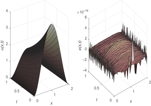
The approximation function $\tilde{u} (x, t)$ (left) and the error function (right) with n = 40 for Example 1

By applying the presented method with n = 20 and α = 0.2, the obtained function $\tilde{u} (x, t)$ is plotted in Figure 2. Moreover, the error of the obtained function $\tilde{u} (x, t)$ is plotted in this figure too. Consumed CPU time for an accurate solution is obtained in just 23.427 seconds. In Table 1, $E_{n, m}^{2} (u)$ is the two-norms of the error for the obtained function $\tilde{u} (x, t)$ ⁠, which is defined as,

E_{n, m}^{2} (u) ≔ {[\sum_{i = 1}^{n} \sum_{j = 1}^{m} {(\tilde{u} ({\hat{τ}}_{i}, t_{j}) - u ({\hat{τ}}_{i}, t_{j}))}^{2}]}^{\frac{1}{2}} .

Figure 2

View large Download slide

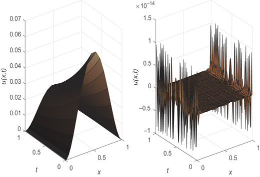
The approximation function $\tilde{u} (x, t)$ (left) and the error function (right) with n = 20 and α = 0.2 for Example 2

Table 1

Example 2: Norms of errors E_n,100(u) for various values of n and α

Α	$E_{4,100}^{2} (u)$	$E_{8,100}^{2} (u)$	$E_{12,100}^{2} (u)$	$E_{16,100}^{2} (u)$
α = 1.2	3.4816e − 15	4.1010e − 15	5.7264e − 15	9.4558e − 15
α = 1.5	3.4191e − 15	4.1058e − 15	6.4447e − 15	9.5015e − 15
α = 1.8	2.4772e − 15	4.3510e − 15	7.4810e − 15	1.1811e − 14

Α	$E_{4,100}^{2} (u)$	$E_{8,100}^{2} (u)$	$E_{12,100}^{2} (u)$	$E_{16,100}^{2} (u)$
α = 1.2	3.4816e − 15	4.1010e − 15	5.7264e − 15	9.4558e − 15
α = 1.5	3.4191e − 15	4.1058e − 15	6.4447e − 15	9.5015e − 15
α = 1.8	2.4772e − 15	4.3510e − 15	7.4810e − 15	1.1811e − 14

From Table 1, it can be seen that norms of errors for various values of n and α appear that the small numbers of n, with that an accurate solution.

Example 3.

We consider the following SFPDEs [29]:

\frac{\partial u (x, t)}{\partial t} = K_{α} \frac{\partial^{α}}{\partial {|x|}^{α}} u (x, t), 0 < x \leq π, 1 < α \leq 2,

(40)

with initial and boundary conditions:

u (x, 0) = \sin (4 x), u (0, t) = u (π, t) = 0,

(41)

Figure 3 shows the approximation function of $\tilde{u} (x, t)$ ⁠, for order of fractional derivative α = 1.25 and ℵ = 1.5 and the time for 0 < t < 1. Observed that if value of α is decreased from 2 to 1 the amplitude of the sinusoidal solution behavior is increased. In Table 2, the values of $\tilde{u} (x, 1)$ in various values of x and n with the value of α = 1.5

Example 4.

We consider the following FPDEs [42, 43]

\frac{\partial u (x, t)}{\partial t} + u (x, t) = \frac{\partial^{α}}{\partial {|x|}^{α}} u (x, t) + s (x, t), 1 < α \leq 2,

(42)

Figure 3

View large Download slide

The approximation function $\tilde{u} (x, t)$ with n = 40 and α = 1.25, 1.5 for Example 3

Table 2

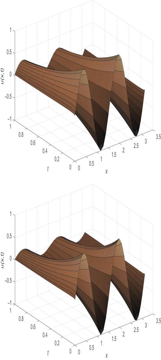
Example 3: The values of $\tilde{u} (x, 1)$ in various values of x and n with the value of α = 1.5

Values of n	n = 11	n = 16	n = 21	n = 26	n = 31
$\tilde{u} (π / 5,1)$	0.099371	0.099576	0.099791	0.099962	0.100035
$\tilde{u} (2 π / 5,1)$	−0.124557	−0.124638	−0.124584	−0.124602	−0.124594
$\tilde{u} (3 π / 5,1)$	0.124557	0.124638	0.124584	0.124602	0.124594
$\tilde{u} (4 π / 5,1)$	−0.099371	−0.099576	−0.099791	−0.099962	−0.100035

Values of n	n = 11	n = 16	n = 21	n = 26	n = 31
$\tilde{u} (π / 5,1)$	0.099371	0.099576	0.099791	0.099962	0.100035
$\tilde{u} (2 π / 5,1)$	−0.124557	−0.124638	−0.124584	−0.124602	−0.124594
$\tilde{u} (3 π / 5,1)$	0.124557	0.124638	0.124584	0.124602	0.124594
$\tilde{u} (4 π / 5,1)$	−0.099371	−0.099576	−0.099791	−0.099962	−0.100035

with initial and boundary conditions:

u (x, 0) = x^{2} {(L - x)}^{2}, 0 < x \leq L, u (0, t) = u (L, t) = 0, 0 \leq t \leq T,

(43)

s (x, t) = \frac{4 e^{- t}}{\cos \frac{π α}{2}} (\frac{3 (x^{4 - α} + {(L - x)}^{4 - α})}{Γ (5 - α)} - \frac{(x^{3 - α} + {(L - x)}^{3 - α})}{Γ (4 - α)} + \frac{(x^{2 - α} + {(L - x)}^{2 - α})}{Γ (3 - α)}) .

The exact solution is of the form u(x, t) = x²(L − x)²e^−t The problem (42) has been solved in [43] by proposed a class of difference scheme based on the parameter spline function and improved matrix transform method. Also, the authors in [42] have solved this problem (42) by proposing a space-time spectral algorithm based on the shifted Jacobi tau technique. To demonstrate the accuracy of our proposed method, in Table 3, compare the absolute errors |u(x_i, 0.1) − u(x_i, 0.1)|, i = 1, …, 9 with the numerical method proposed in [42, 43] and our results for various choices of α.

Table 3

Example 4: Comparison of absolute errors of our scheme with scheme in [42, 43]

Method of [42]				Method of [43]			The presented method
x	α = 1.2	α = 1.5	α = 1.8	α = 1.2	α = 1.5	α = 1.8	α = 1.2	α = 1.5	α = 1.8
0.2	1.54 e-12	3.78 e-11	4.34 e-11	1.61 e-3	1.42 e-3	7.24 e-4	0.1055e-12	0.9843e-12	1.9413e-12
0.4	1.44 e-10	8.64 e-11	1.37 e-10	1.42 e-3	1.02 e-3	5.74 e-4	1.47905e-12	3.9820e-12	2.3070e-12
0.6	1.63 e-10	1.54 e-10	1.48 e-10	8.75 e-4	7.49 e-4	4.12 e-4	3.3255e-12	5.0410e-12	9.1279e-13
0.8	1.30 e-10	2.10 e-10	1.55 e-10	7.50 e-4	6.16 e-4	3.22 e-4	1.1055e-12	3.0410e-12	2.3986e-12
1.0	1.89 e-10	2.21 e-10	2.19 e-10	7.13 e-4	5.76 e-4	2.95 e-4	2.1152e-12	1.0010e-12	8.3765e-12
1.2	2.48 e-10	1.94 e-10	2.53 e-10	7.50 e-4	6.16 e-4	3.22 e-4	7.0055e-12	1.0410e-13	5.1819e-12
1.4	1.73 e-10	1.51 e-10	1.74 e-10	8.75 e-4	7.49 e-4	4.12 e-4	1.3498e-12	1.2430e-12	2.2781e-12
1.6	5.11 e-11	9.89 e-11	6.21 e-11	1.42 e-3	1.02 e-3	5.74 e-4	6.245e-12	3.0410e-12	5.2410e-12
1.8	3.43 e-11	3.72 e-11	3.08 e-11	1.61 e-3	1.42 e-3	7.24 e-4	1.1055e-13	3.0410e-12	1.3452e-12

Method of [42]				Method of [43]			The presented method
x	α = 1.2	α = 1.5	α = 1.8	α = 1.2	α = 1.5	α = 1.8	α = 1.2	α = 1.5	α = 1.8
0.2	1.54 e-12	3.78 e-11	4.34 e-11	1.61 e-3	1.42 e-3	7.24 e-4	0.1055e-12	0.9843e-12	1.9413e-12
0.4	1.44 e-10	8.64 e-11	1.37 e-10	1.42 e-3	1.02 e-3	5.74 e-4	1.47905e-12	3.9820e-12	2.3070e-12
0.6	1.63 e-10	1.54 e-10	1.48 e-10	8.75 e-4	7.49 e-4	4.12 e-4	3.3255e-12	5.0410e-12	9.1279e-13
0.8	1.30 e-10	2.10 e-10	1.55 e-10	7.50 e-4	6.16 e-4	3.22 e-4	1.1055e-12	3.0410e-12	2.3986e-12
1.0	1.89 e-10	2.21 e-10	2.19 e-10	7.13 e-4	5.76 e-4	2.95 e-4	2.1152e-12	1.0010e-12	8.3765e-12
1.2	2.48 e-10	1.94 e-10	2.53 e-10	7.50 e-4	6.16 e-4	3.22 e-4	7.0055e-12	1.0410e-13	5.1819e-12
1.4	1.73 e-10	1.51 e-10	1.74 e-10	8.75 e-4	7.49 e-4	4.12 e-4	1.3498e-12	1.2430e-12	2.2781e-12
1.6	5.11 e-11	9.89 e-11	6.21 e-11	1.42 e-3	1.02 e-3	5.74 e-4	6.245e-12	3.0410e-12	5.2410e-12
1.8	3.43 e-11	3.72 e-11	3.08 e-11	1.61 e-3	1.42 e-3	7.24 e-4	1.1055e-13	3.0410e-12	1.3452e-12

5. Conclusion

In the present paper, we developed an efficient and accurate method for solving SFPDE. Applying the MOL together with the pseudospectral discretization method converts the SFPDE to the system of ordinary differential equations. Choosing the shifted Jacobi functions as a test basis with special parameters a, b gives us this opportunity to obtain the left- and right-sided fractional differentiation matrices for this basis exactly.

Four examples have been solved, and the results are reported. These results show that our method is efficient and provides accurate results, whereas a small number of JG nodes are used based on the collocation method. Obtaining some theoretical estimates for the approximation errors would be desirable.

References

1.

Debnath

L

.

Recent applications of fractional calculus to science and engineering

.

Int J Math Math Sci

.

2003

;

2003

(

54

):

3413

-

42

.

Google Scholar

Crossref

2.

Gorenflo

R

,

Mainardi

F

.

Fractional oscillations and Mittag-Leffler functions

:

Citeseer

;

1996

.

Google Scholar

3.

Hilfer

R

. Applications of fractional calculus in physics. In:

Hilfer

R

, editer.

Applications of fractional calculus in physics

:

Published by World Scientific Publishing

;

2000

. ISBN

[PubMed]

.

Google Scholar

Crossref

4.

Adam

M

.

Advances in fractional calculus: theoretical developments and applications in physics and engineering

;

2008

.

Google Scholar

5.

George

MZ

.

Hamiltonian chaos and fractional dynamics

:

Oxford University Press on Demand

;

2005

.

Google Scholar

6.

Bratsos

AG

.

The solution of the two-dimensional sine-Gordon equation using the method of lines

.

J Comput Appl Math

.

2007

;

206

(

1

):

251

-

77

.

Google Scholar

Crossref

7.

Dehghan

M

,

Shakeri

F

.

Method of lines solutions of the parabolic inverse problem with an overspecification at a point

.

Numer Algorithm

.

2009

;

50

(

4

):

417

-

37

.

Google Scholar

Crossref

8.

Haq

S

. et al.

Meshless method of lines for the numerical solution of generalized Kuramoto-Sivashinsky equation

.

Appl Math Comput

.

2010

;

217

(

6

):

2404

-

13

.

Google Scholar

9.

Northrop

PWC

, et al.

A robust false transient method of lines for elliptic partial differential equations

.

Chem Eng Sci

.

2013

;

90

:

32

-

39

.

Google Scholar

Crossref

10.

Shakeri

F

,

Dehghan

M

.

The method of lines for solution of the one-dimensional wave equation subject to an integral conservation condition

.

Comput Math Appl

.

2008

;

56

(

9

):

2175

-

88

.

Google Scholar

Crossref

11.

Quan

S

.

A meshless method of lines for the numerical solution of KdV equation using radial basis functions

.

Eng Anal Bound Elem

.

2009

;

33

(

10

):

1171

-

80

.

Google Scholar

12.

Voss

DA

,

Abdul-Qayyum

MK

.

Time-stepping algorithms for semidiscretized linear parabolic PDEs based on rational approximants with distinct real poles

.

Adv Comput Math

.

1996

;

6

(

1

):

353

-

63

.

Google Scholar

Crossref

13.

Hamdi

S

,

Schiesser

WE

,

Griffiths

GW

.

Method of lines

.

Scholarpedia

.

2007

;

2

(

7

):

2859

.

Google Scholar

Crossref

14.

James

MH

.

Method of lines approach to the numerical solution of conservation laws

.

Technical Report

,

NM

:

Los Alamos Scientific Lab

:

1979

.

Google Scholar

15.

Saucez

P

, et al.

Method of lines study of nonlinear dispersive waves

.

J Comput Appl Math

.

2004

;

168

(

1-2

):

413

-

23

.

Google Scholar

Crossref

16.

Hamdi

S

, et al.

Method of lines solutions of the extended Boussinesq equations

.

J Comput Appl Math

.

2005

;

183

(

2

):

327

-

42

.

Google Scholar

Crossref

17.

White

RE

,

Subramanian

VR

.

Method of lines for parabolic partial differential equations

.

Computational methods in chemical engineering with maple

:

Springer

;

2010

,

353

-

505

.

Google Scholar

Crossref

18.

Schiesser

WE

.

Method of lines PDE analysis in biomedical science and engineering

:

John Wiley and Sons

;

2016

.

Google Scholar

Crossref

19.

Causley

MF

, et al.

Method of lines transpose: high order L-stable \mathcalO(N) schemes for parabolic equations using successive convolution

.

SIAM J Numer Anal

.

2016

;

54

(

3

):

1635

-

52

.

Google Scholar

Crossref

20.

Yang

Q

, et al.

A finite volume scheme with preconditioned Lanczos method for two-dimensional space-fractional reaction–diffusion equations

.

Appl Math Model

.

2014

;

38

(

15-6

):

3755

-

62

.

Google Scholar

21.

Liu

Y

, et al.

Time two-mesh algorithm combined with finite element method for time fractional water wave model

. In:

Int J Heat Mass Tran

.

2018

;

120

:

1132

-

45

.

Google Scholar

Crossref

22.

Bu

W

,

Tang

Y

,

Yang

J

.

Galerkin finite element method for two-dimensional Riesz space fractional diffusion equations

.

J Comput Phys

.

2014

;

276

:

26

-

38

.

Google Scholar

Crossref

23.

Feng

LB

, et al.

Stability and convergence of a new finite volume method for a two-sided space-fractional diffusion equation

.

Appl Math Comput

.

2015

;

257

:

52

-

65

.

Google Scholar

24.

Liu

F

,

Anh

V

,

Turner

I

.

Numerical solution of the space fractional Fokker–Planck equation

.

J Comput Appl Math

.

2004

;

166

(

1

):

209

-

19

.

Google Scholar

Crossref

25.

Meerschaert

MM

,

Tadjeran

C

.

Finite difference approximations for fractional advection–dispersion flow equations

.

J Comput Appl Math

.

2004

;

172

(

1

):

65

-

77

.

Google Scholar

Crossref

26.

Shen

J

,

Tang

T

,

Wang

LL

.

Spectral methods: algorithms, analysis and applications

:

Springer Science & Business Media

;

2011

,

41

.

Google Scholar

Crossref

27.

Schiesser

WE

,

Griffiths

GW

.

A compendium of partial differential equation models: method of lines analysis with Matlab

:

Cambridge University Press

;

2009

.

Google Scholar

Crossref

28.

Esmaeili

S

,

Shamsi

M

,

Luchko

Y

.

Numerical solution of fractional differential equations with a collocation method based on Müntz polynomials

.

Comput Math Appl

.

2011

;

62

(

3

):

918

-

29

.

Google Scholar

Crossref

29.

Yang

Q

,

Liu

F

,

Turner

I

.

Numerical methods for fractional partial differential equations with Riesz space fractional derivatives

.

Appl Math Model

.

2010

;

34

(

1

): pp.

200

-

18

.

Google Scholar

Crossref

30.

Esmaeili

S

,

Shamsi

M

.

A pseudo-spectral scheme for the approximate solution of a family of fractional differential equations

.

Commun Nonlinear Sci Numer Simulat

.

2011

;

16

(

9

):

3646

-

54

.

Google Scholar

Crossref

31.

Zayernouri

M

,

George

EK

.

Fractional sturm–liouville eigen-problems: theory and numerical approximation

.

J Comput Phys

.

2013

;

252

:

495

-

517

.

Google Scholar

Crossref

32.

Chen

S

,

Shen

J

,

Wang

LL

.

Generalized Jacobi functions and their applications to fractional differential equations

.

Math Comput

.

2016

;

85

(

300

):

1603

-

38

.

Google Scholar

Crossref

33.

Zayernouri

M

,

Ainsworth

M

,

George

EK

.

A unified Petrov–Galerkin spectral method for fractional PDEs

.

Comput Methods Appl Mech Eng

.

2015

;

283

:

1545

-

69

.

Google Scholar

Crossref

34.

Zayernouri

M

,

Ainsworth

M

,

George

EK

.

Tempered fractional sturm–liouville EigenProblems

.

SIAM J Sci Comput

.

2015

;

37

(

4

):

A1777

–

1800

.

Google Scholar

Crossref

35.

Zayernouri

M

,

George

EK

.

Discontinuous spectral element methods for time-and space-fractional advection equations

.

SIAM J Sci Comput

.

2014

;

36

(

4

):

B684

-

707

.

Google Scholar

Crossref

36.

Zayernouri

M

,

George

EK

.

Exponentially accurate spectral and spectral element methods for fractional ODEs

.

J Comput Phys

.

2014

;

257

:

460

-

80

.

Google Scholar

Crossref

37.

Zayernouri

M

,

George

EK

.

Fractional spectral collocation method

.

SIAM J Sci Comput

.

2014

;

36

(

1

):

A40

-

62

.

Google Scholar

Crossref

38.

Zayernouri

M

,

George

EK

.

Fractional spectral collocation methods for linear and nonlinear variable order FPDEs

.

J Comput Phys

.

2015

;

293

:

312

-

38

.

Google Scholar

Crossref

39.

Zayernouri

M

, et al.

Spectral and discontinuous spectral element methods for fractional delay equations

.

SIAM J Sc. Comput

.

2014

;

36

(

6

):

B904

-

29

.

Google Scholar

Crossref

40.

Zhang

Z

,

Zeng

F

,

George

EK

.

Optimal error estimates of spectral Petrov–Galerkin and collocation methods for initial value problems of fractional differential equations

.

SIAM J Numer Anal

.

2015

;

53

(

4

):

2074

-

96

.

Google Scholar

Crossref

41.

Meerschaert

MM

,

Tadjeran

C

.

Finite difference approximations for two-sided space-fractional partial differential equations

.

Appl Numer Math

.

2006

;

56

(

1

):

80

-

90

.

Google Scholar

Crossref

42.

Bhrawy

AH

,

Zaky

MA

.

A method based on the Jacobi tau approximation for solving multi-term time-space fractional partial differential equations

.

J Comput Phys

.

2015

;

281

:

876

-

95

.

Google Scholar

Crossref

43.

Zhang

Y

,

Ding

H

.

Improved matrix transform method for the Riesz space fractional reaction dispersion equation

.

J Comput Appl Math

.

2014

;

260

:

266

-

80

.

Google Scholar

Crossref

2021

Mushtaq Ali, Mohammed Almoaeet and Basim Karim Albuohimad

Published in Arab Journal of Mathematical Sciences. Published by Emerald Publishing Limited. This article is published under the Creative Commons Attribution (CC BY 4.0) licence. Anyone may reproduce, distribute, translate and create derivative works of this article (for both commercial and non-commercial purposes), subject to full attribution to the original publication and authors. The full terms of this licence may be seen at http://creativecommons.org/licences/by/4.0/legalcode

Numerical simulation method of lines together with a pseudospectral method for solving space-time partial differential equations with space left- and right-sided fractional derivative

1. Introduction

2. Preliminaries and definitions

2.1 Jacobi–Gauss nodes

3. Th presented pseudospectral discretization method

3.1 On the derivation of the left and right fractional differentiation matrices

4. Numerical results and comparisons

5. Conclusion

References

New and popular articles

Email Alerts

Cited By

Numerical simulation method of lines together with a pseudospectral method for solving space-time partial differential equations with space left- and right-sided fractional derivative

1. Introduction

2. Preliminaries and definitions

2.1 Jacobi–Gauss nodes

3. Th presented pseudospectral discretization method

3.1 On the derivation of the left and right fractional differentiation matrices

4. Numerical results and comparisons

5. Conclusion

References

New and popular articles

Email Alerts

Suggested Reading

Recommended for you

Cited By

Sharing Unavailable