Surface reconstruction from point cloud scans is crucial in 3D vision and graphics. Recent approaches focus on training deep-learning (DL) models to generate representations through learned priors. These models use neural networks to map point clouds into compact representations and then decode these latent representations into signed distance functions (SDFs). Such methods rely on heavy supervision and incur high computational costs. Moreover, they lack interpretability regarding how the encoded representations influence the resulting surfaces. This work proposes a computationally efficient and mathematically transparent Green Learning (GL) solution. We name it the lightweight point-cloud surface reconstruction (LPSR) method. LPSR reconstructs surfaces in two steps. First, it progressively generates a sparse voxel representation using a feedforward approach. Second, it decodes the representation into unsigned distance functions (UDFs) based on anisotropic heat diffusion. Experimental results show that LPSR offers competitive performance against state-of-the-art surface reconstruction methods on the FAMOUS, ABC, and Thingi10K datasets at modest model complexity.
1 Introduction
Surface reconstruction from point cloud scans is critical in 3D vision and graphics. It finds applications in augmented and virtual reality (AR/VR), cultural heritage preservation, building information modeling (BIM), etc. Surface reconstruction has recently gained attention in 3D AI-generated content (AIGC). One inherent challenge in surface reconstruction from point clouds stems from the ill-posed nature of reconstructing continuous surfaces from discrete points. The fact that infinitely many possible surfaces can pass through the input points makes it an open problem with no universally optimal solution.
Early research in this field [6, 7, 13, 16, 21, 28, 29, 48] employed unsu-pervised solutions, where prior knowledge and assumptions (e.g., smoothness, consistent normal directions) were heuristically designed to approximate an optimal solution. Their reconstruction quality is somehow limited.
More recent efforts leverage supervision by pairing point clouds and their surfaces, allowing surface reconstruction models to gain prior knowledge via supervised learning. They use deep neural networks to map point clouds into compact representations and then decode these latent representations into signed distance functions (SDFs). The supervised deep-learning (DL) methodology has become the dominant one nowadays [3, 14, 18, 35, 36, 38, 39, 41, 42, 44, 45, 47]. DL models have the “encoder” and the “decoder” modules applied to those 3D shape modeling or generative tasks. The former transforms point clouds into latent vectors while the latter converts latent vectors to output iso-surfaces [51]. Despite the superior performance of supervised models over unsupervised ones, several challenges remain unresolved.
The first one is the interpretability of supervised DL models. Point clouds are encoded into high-dimensional latent spaces and decoded into a signed distance field (SDF) using convolutional neural networks (CNNs) or transformer layers. The latent representations are difficult to explain, and the contributions of various layers are unclear due to the black-box nature of DL models. Lack of interpretability may lead to reconstruction failures and hinder effective analysis of the model’s generalizability. Moreover, it complicates the conditioning process in 3D generation and reconstruction. To address this shortcoming, we propose an explainable method that yields explainable results step by step. The second one is the training and inference complexity and model sizes. Although GPUs can accelerate inference, DL models demand significant memory and computational resources. Furthermore, they need a large amount of training data. This is a concern since the sample numbers in 3D object datasets are much smaller than those in 2D image datasets (e.g., 50K samples in ShapeNet[8] vs. 1.4M images in ImageNet[12]).
To tackle interpretability and complexity, we propose a lightweight point cloud surface reconstruction (LPSR) method in this work. It extends our previous work, GPSR [59]. LPSR enhances the heat diffusion module in GPSR and employs a supervised learning paradigm to boost the performance. LPSR features a feedforward-designed encoder and a PDE-based decoder with mathematical transparency. The encoded representation has a clear physical meaning in controlling the surface shape, and it can be decoded at different grid resolutions to produce different levels of detail.
The main contributions of this work are summarized below.
We propose a lightweight supervised learning pipeline that progressively constructs voxel representations across multi-resolutions. Feature derivation, selection, and decision-making are all implemented in a feedforward and statistical approach.
We design a decoder that leverages geometric priors and adopts anisotropic heat diffusion to generate surfaces from representations with modest memory in an unsupervised manner. It accurately maps the representation to the 3D distance field.
We conduct experiments on two 3D object datasets to demonstrate that LPSR achieves competitive performance against state-of-the-art (SOTA) surface reconstruction methods with lower memory consumption and at a smaller model size.
2 Related Work
Surface reconstruction methods can be classified into two categories: unsuper-vised and supervised. We provide a brief review of them below.
2.1 Unsupervised Surface Reconstruction Methods
Early unsupervised methods utilized combinatorial techniques, such as De-launay triangulation or Voronoi diagrams, to directly infer point connectivity. Notable examples include ball-pivoting [4] and power crust [1]. While these methods are computationally less complex, they often struggle with accuracy and cannot guarantee watertight surfaces.
On the other hand, implicit function methods solve an underdetermined partial differential equation (PDE) system, where the solution represents the target implicit surface in the 3D space. To mitigate the ill-posedness of the system, geometric priors or constraints such as point normals and surface smoothness are typically required. A prominent example is the Screened Poisson method [28, 29]. It formulates the Poisson equation by enforcing consistency between SDF gradients and point normals. This method is attractive due to its accuracy and relatively low computational cost. However, it is sensitive to input data noise and point normals’ accuracy. To address them, the iPSR method [22] enhances the Poisson surface reconstruction process by iteratively updating oriented normals and refining the surface reconstruction at each iteration. Xiao et al. [48] improve the orientation of normals by incorporating an iso-value constraint in the Poisson equations. The PGR method [33] eliminates the need for normals, treats surface normals and element areas as unknown parameters, and optimizes these parameters to achieve better surface representation.
Unsupervised surface reconstruction methods rely on heuristic assumptions to approximate optimal solutions. They ignore specific requirements of certain scenarios (e.g., objects, indoor scenes, outdoor environments, and human faces). Therefore, their performance is generally inferior to that of supervised methods.
2.2 Supervised Surface Reconstruction Methods
Supervised surface reconstruction methods utilize machine learning models to yield the UDF/SDF or the occupancy grid. We examine them from two angles below.
Representations. Since 3D UDF/SDF/occupancy grids can be redundant and less informative, alternative 3D representations have been introduced to create more compact and informative ones. One approach solves the problem in the point domain [5, 14, 37, 2]. For example, Points2Surf [14] employs a PointNet-based network to predict SDF values in the point domain. Similarly, DeepSDF [37] utilizes an auto-decoder to optimize randomly initialized latent vectors at each point. While solving the problem in the point domain is memory efficient, the positional information computation can be expensive. Sparse voxel representations, widely adopted by SOTA methods [23, 24, 39, 50], store the positional information in voxel grids. This strategy alleviates the burden on decoders but has relatively high memory consumption. Triplanes [43] and similar projective representations [34] introduce a novel representation that mitigates the memory concerns associated with voxel grids. [43] utilizes a multilayer perceptron (MLP) to decode 3D grids from projected feature planes, though its interpretability may be limited. Lastly, several methods focus on predicting the UDF [41, 57, 55, 11, 15], which then requires conversion to SDF or direct extraction of an non-watertight surface.
Architectural Issues. Early supervised methods adopted an end-to-end optimized neural network [14, 37] to generate point-wise or voxel-wise SDFs. However, these approaches lack interpretability, exhibit poor cross-dataset performance, and frequently result in failure cases. GeoUDF [41] decomposes the problem into a sequence of modules to enhance interpretability. Huang et al. [23, 24] replace B-spline bases with learned neural kernel bases in the screened Poisson method, which achieves SOTA performance with partial ex-plainability. These methods rely on deep neural networks to predict various meta-information, such as normals and octree structures. Another method is based on iterative online training including Neural-Pull [3], CAP-UDF [57, 55], and Neural-IMLS [46]. Neural-Pull [3] minimizes the distance between query points and predicted SDF or UDFs. These methods do not rely on training sets from external data, thus avoiding potential biases. However, online training can be computationally demanding and carries the risk of producing non-converged results.
Despite their notable performance on specific test sets, DL-based methods demand substantial computational resources and face interpretability issues. Unexpected failures may occur when they are applied to unseen data. Consequently, there is a need for a transparent and lightweight surface reconstruction method.
2.3 Green Learning
This work adopts the Green Learning (GL) paradigm, initially proposed by Kuo et al. [31, 32], to mitigate computational efficiency and interpretability concerns. Green Learning has emerged as an eco-conscious approach within machine learning, emphasizing efficiency and a reduced carbon footprint during model operations. Several core features distinguish this paradigm. It promotes the development of models that are compact in size and have low computational complexity during both training and inference phases. Furthermore, GL is founded on a modularized design principle that enhances mathematical transparency and theoretical explainability.
Specifically, GL reduces the training costs of backpropagation by adopting a purely feedforward training scheme. It employs a modular design that decomposes the whole machine-learning problem into manageable sub-problems, each solved by a transparent learning model. This approach reduces the model size and training/inference complexity and facilitates a theoretically interpretable process across various applications.
Green learning has been applied to a range of point cloud processing tasks. Notable models like PointHop [54], PointHop++ [53], R-PointHop [25], GISP [52], PCRP [27], SPA [26] have proven effective in handling various point cloud processing challenges, including 3D classification, registration, semantic segmentation, and retrieval.
3 Proposed LPSR Method
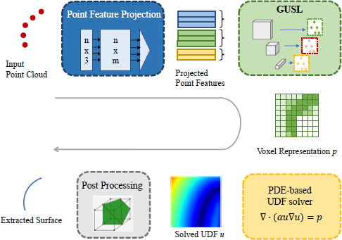
The proposed Learning-based Point Surface Reconstruction (LPSR) method, as illustrated in Figure 1, employs a sequential modular approach to transform an input point cloud into an unsigned distance field (UDF). It consists of four cascaded modules, as depicted in Figure 1. They are: 1) Point Feature Projection, 2) Sparse Green U-Shaped Learning (GUSL), 3) PDE-based UDF Solution, and 4) Post Processing. In the first module, a point feature projection operator is employed to extract point features, which are voxelized through voxel-wise aggregation. The second module progressively learns the representation in a feedforward manner. The representation output from Module 2 is used as the input to Module 3, which solves a partial differential equation (PDE) for the UDF. Finally, after the sign assignment, Module 4 uses a marching-cubes algorithm to obtain the distance field. For clarity and logical progression in explanation, the methodological description begins with the Point Feature Projection module, followed by the detailed exposition of the PDE-based UDF decoder module. The Sparse GUSL framework is discussed further in Section 3.3, and the Post Processing steps are elaborated in Section 3.4.
3.1 Point Feature Projection
In this module, the input point clouds are voxelized and yield voxel features in an unsupervised process. As discussed in Section 2.2, a voxel grid is favored among various representations because it contains positional information, and no positional decoder is needed. We employ a sparse voxel grid to avoid excessive memory consumption, considering only occupied voxels.
To convert point features to voxel features, we voxelize an input point cloud into a 3d grid of size d × d × d. Within each voxel cube, we recenter the points using the voxel geometry center. The recentered points inside the voxel can be denoted as {p1,p2, …, pn} ⊆ ℝ3. To align the dimension across different voxels, we introduce a PoinNet-like structure [40]. A recentered point Pi is projected into a high-dimensional feature fi using a shared weights W and bias b:
where σ(·) is a non-linear activation function, specifically ReLU. Then, a maximum aggregation function produces a voxel feature F by:
The major difference between our method and PointNet is that the weights W and biases b in our module are purely based on random initialization and do not require supervision for adjustment. We choose a large feature dimension and rely on a feature selection module to identify powerful features, as discussed in Section 3.2.
3.2 Heat-equation-based Surface Decoder
Motivation. The motivation behind applying a PDE-based decoder is to parameterize the UDF/occupancy field into an explainable feature space, thereby avoiding the black box decoding processes typical of MLPs or other decoding layers. This idea is shared by a group of supervised works [23, 24]. Considering the SDF/UDF is continuous in space and monotonic in empty regions, one can parameterize it to some compact representations. Differ from [24] using popular B-spline or Fourier bases to represent the SDF, we opt to use a temperature grid to mimic the UDF and control the grid by parameterizing the boundary conditions (e.g., temperature or heat flux). The advantages of using a heat-equation solution as the UDF are outlined below:
The steady-state solution of the heat equation forms a smooth and continuous 3D grid, supporting re-scaling using the finite element method (FEM).
Temperature values in empty voxels follow a monotonic change, with values falling between the lowest and highest temperature ranges.
The temperature is controlled by the magnitude and spatial position of the heat source / flux, which is inherently differentiable.
This approach has proven efficient in our previous work, GPSR [59].
Implementation Details. Given a discrete 3D grid, our goal is to establish a heat flux or temperature control function q(x) and seek the steady state solution u(x) to the heat equation, Eq. (3), which will serve as the UDF:
where D is the diffusion coefficient, is set to 0 in the steady state when u(x) does not change w.r.t. to time t.
Unlike our previous GPSR method, which treats the diffusion coefficient D as a constant value, we set the D as a dependent variable of u by
where α is a scalar parameter. This modification leads to the establishment of a more accurate steady-state equation:
which offers a more precise solution that converges to the UDF. We then discretize Eq. (5) into a matrix form:
where ⊙ denotes the Hadamard product. Gx, Gy, Gz are matrix form of discrete gradient operator along x, y, z directions, respectively. The solution u is the flattened UDF vector in the 3D grid. The q is the vector representing the heat source/flux controlling the shape of the UDF.
The following two constraints must be satisfied to guarantee a converged steady-state solution.
The boundary condition is set to Neumann boundary condition with zero heat flux, indicating no heat exchange with the outside environment at the boundary.
The vector q has a zero-sum, indicating that the net heat flux entering and leaving the system is zero.
Considering the non-linear parabolic PDE, Eq. (6), cannot be directly solved, we treat it as an optimization problem and use the gradient descent method to solve it iteratively. The initial guess for optimization is the qpred obtained from the XGBoost regressor. We use the iterative approach to solve the PDE for upred, the output UDF.
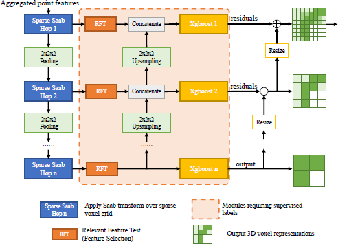
3.3 Sparse Green U-Shaped Learning (GUSL) Model
The GUSL model is the critical module that maps the aggregated point features into a compact representation using the Green Learning paradigm. As shown in Figure 2, it follows a U-shape pipeline and progressively yields representations at different grid resolutions. The framework comprises three modules for each resolution: unsupervised Saab feature construction, semi-supervised feature selection, and supervised decision learning. We will introduce these modules in the following.
1) Sparse Saab Transform. To yield decorrelated representation features from the input voxel features, a channel-wise (c/w) Saab Transform [10, 32] is applied on each local voxel neighborhood to derive its new representation in terms of Saab coefficients in an unsupervised manner. Given the sparse nature of the 3D voxel representation, we only apply the c/w-Saab transform over the occupied neighborhood, following a similar scheme of sparse convolution [17]. Using the n-hop c/w-Saab transform layers increase the spectrum resolution to capture spatial correlations. The 3-layer features are sent to the multi-grid feature selection and decision learning module.
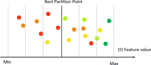
2) Feature Selection. Reducing the input feature dimension is essential to achieve a lightweight model. Therefore, we introduce a semi-supervised feature selection technique called the Relevant Feature Test (RFT) [49]. As shown in Figure 3, for a given 1D input feature, samples are ordered by their feature values, and the sample maximum and minimum bind the feature dimension. The representation is then partitioned into two sub-intervals at a set of uniformly spaced points between the maximum and minimum. We compute the mean values of the samples in the left and right sub-intervals, find the point that minimizes the weighted mean-squared error (MSE), and define this MSE value as the RFT cost for that representation. The RFT cost indicates the effectiveness of the representation in reducing regression errors. We select the top k features with the most discriminant power and discard the rest. “semi-supervised” means only a small subset of labels among the training samples are required in the feature selection process.
One challenge with incorporating supervision in our method is the absence of backpropagation, which prevents traditional gradient-based learning. We employ an indirect labeling approach to address this by utilizing outputs from the PDE-based Module 3. Specifically, we pass the ground truth UDF ugt pass through Eq. (5) introduced in Section 3.3 under different grid resolutions. In Eq. (5), α is a scalar coefficient, u(x) represent the UDF at position x and q(x) denotes the resulting representation. This process yields a set of ground truth representation labels corresponding to various resolutions. These labels are then used to effectively guide the feature selection process without relying on backpropagation.
3) Decision Learning. The selected features predict each voxel’s representations qpred. These predictions are made using a group of progressive XGBoost regressors [9]. The XGBoost model at the coarsest grid level (Hop n) produces the coarse prediction for the representation voxel, while those at finer grid levels predict the corresponding residuals , between the ground truth and the previous predictions.
As discussed in the previous paragraph, directly inferring the upred from Ppred involves solving a non-linear PDE in each training iteration, which can be computationally expensive. To address this, we define an indirect loss for the representation term q:
In addition, when the qpred is close to the ground truth, a correction term is required to respect the PDE. In this case, we solve the PDE and define a loss for the PDE solution upred:
where upred is the solution to the heat propagation equation, Eq. (3), given representation q. The overall learning objective function can be expressed as:
The parameter, λ, is initially set to 0 in the training and gradually increases to a preset value as the iteration progresses.
3.4 Post Processing
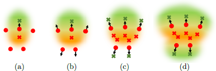
In this module, we aim to convert the unsigned distance field into a surface by assigning a sign to the UDF upred and applying a marching cube to the recovered SDF spred. To infer the sign of the predicted distance field upred, we follow the approach used in GPSR [59]. As shown in Figure 4, the process of converting UDF to SDF involves a forward heat propagation process across a 3D temperature grid T through the following steps:
Step 1: Identify all voxels intersected by the surface in a unit 3D space with resolution d × d × d. A voxel is considered occupied (intersected by the surface) if its predicted unsigned distance is less than 0.5 * s, where s = 1/d.
Step 2: Compute the unit-length normal direction vector n for each occupied voxel by determining the direction of the steepest gradient in UDF.
Step 3: Arbitrarily select an occupied voxel pi = (xi,yi,Zi) with normal direction ni as the starting point. The sign of ni can be arbitrarily assigned.
Step 4: Compute 2 candidate locations 11i and l2i for each point pi as follows:
(10)(11)Append l1i, l2i to two sets P and N, respectively.
Step 5: Designate all locations in P and N as constant heat sources with temperature +1 and sinks with temperature -1, respectively. Perform a forward heat diffusion iteration over T, as demonstrated in Figure 4 (a).
Step 6: For each adjacent occupied voxel pj·, append l1j to P if T(11j) > 0, and to N if T(11j) < 0; apply the same criteria to l2j·. This operation is demonstrated in Figure 4 (b).
Step 7: Repeat Step 5, cycling through each voxel until all occupied voxels are processed, as shown in Figures 4 (c) and (d).
Following the propagation of all occupied voxels, the signs from the temperature field T are extracted. The SDF spred is calculated as follows:
where ⊙ denotes the element-wise product. Finally, the marching cubes algorithm is applied to spred to extract the surface.
Our surface extraction method shares similarities with MeshUDF [20] in determining the sign of the distance field. However, there are distinct differences between the two approaches. MeshUDF utilizes the projection of neighboring gradient vectors to compute the vote values for sign determination. While our method is a more straightforward approach by assigning preset temperatures to specific locations and utilizing a heat transmission process to infer values throughout the grid.
4 Experiments
4.1 Experimental Settings
We compare the performance of various surface reconstruction methods on three datasets: FAMOUS [14], ABC [30], and Thingi10K [58]. They have various types of degradation, including missing parts and different noise levels. The input point cloud sets are categorized into three types: noise-free, original, and extra-noise, with the variance of noise set to 0.00L, 0.01L, and 0.05L, respectively. The L denotes the largest side of the mesh bounding box. The model is trained over the ABC [30] dataset following a similar setting to [14].
We compare our LPSR method with several other surface reconstruction methods, including Screened Poisson Reconstruction (SPR) [29], PGR [33], Neural-Pull [3], Points2surf [14], PCPNet [19], POCO [5], NKSR [24], Geo-UDF [41], CAP-UDF [55], and LevelSetUDF [56]. SPR and PGR are unsu-pervised, non-data-driven methods that do not incorporate learning modules, while the remaining seven are powered by learning-based approaches. It is worth noting that PCPNet generates oriented point normals as outputs, and SPR is used to yield its surface for fair comparison. SPR+PCPNet denotes the resulting method. Experimental results for different point set categories are reported by following the configuration settings specified by each method’s papers for consistency and comparability.
The reconstruction quality is measured by the similarity between the ground truth mesh, MeshGT, and the reconstructed mesh surface, Meshrec. We normalize both meshes into unit size and uniformly sample 10,000 points to yield point cloud sets, PCgt and PCrec. Following existing works [33, 14], we use the symmetric Chamfer distance (CD) and the Hausdorff distance (HD) between PCgt and PCrec, and the symmetric mesh cosine similarity (CS) between MeshGT and Meshrec as three quality metrics. For a comprehensive assessment of the reconstruction quality, F-score (F-S.) and normal consistency (N.C.) are used. Following the existing work of [24], the F-score adopt a threshold of 1% for evaluation.
We normalize all input point clouds to a unit scale within the range [0, 1]. The point clouds are then voxelized with a resolution of 256x256x256. The point feature dimension is set to 48. A three-hop sparse GUSL module is applied, with each Saab transform conducted over a window size of 3x3x3. Pooling and upsampling operations are set with a stride of 2. The feature selection module ensures that the input features to each XGBoost model are reduced to k = 256.
4.2 Quantitative Comparison of Reconstructed Surface Quality
The experimental results for the FAMOUS [14], ABC [30], and Thingi1OK [58] datasets are presented in Tables 1, 2, and 3, respectively. The best and second-best results are highlighted in bold and underlined, respectively. Additionally, to provide a comparative analysis of several leading methods, the F-score and normal consistency across these three datasets are detailed in Tables 4, 5, and 6, respectively.
For the FAMOUS dataset, LPSR significantly improved the performance of our previous work, GPSR. We also see a reduction in the Chamfer and the Hausdorff distances in all three datasets. This is attributed to the in troduced supervision. LPSR employs supervision to control the heat equation, leading to finer distance fields and better handling of various distortions. POCO [5], NKSR [24], Geo-UDF[41], and CAP-UDF[55] exhibit competitive performance in terms of Chamfer distance and Hausdorff distance under noise-free conditions. Among them, POCO excels in robustness against noisy and degraded inputs. On the other hand, it demands a high memory cost since it uses query points to describe the occupancy map. NKSR [24] offers impressive performance on the FAMOUS dataset. However, its accuracy relies on the orientation of input point normals, which can be problematic with noisy inputs in the ABC and Thingi10k datasets.
Regarding UDF-based methods [41, 55, 56], they display excellent performance under noise-free conditions. However, their mesh cosine similarity scores are typically lower than those achieved by other methods. This lower performance can be attributed to the fact that UDF-reconstructed surfaces are generally non-watertight and their surface normals are poorly aligned. These factors significantly impact the mesh cosine similarity of their outputs.
4.3 Complexity Comparison
The complexity is measured over the FAMOUS dataset with noise-free inputs. The model sizes, the computational complexity (in terms of floating operation counts, or FLOPs), and the peak memory requirement are measured by taking the average for the input point clouds. For a fair comparison, the output resolution for most methods are typically set to 256, if possible.
Table 7 compares model sizes, the computational complexity (in terms of floating operation counts, or FLOPs), the peak memory requirement of LPSR, and two unsupervised and seven supervised methods. LPSR exhibits the lowest computational complexity and maintains a notably small model size among all the supervised methods evaluated. Specifically, LPSR’s model size is 23 times smaller and its total FLOPs are 28 times lower than those of the POCO method.
The low FLOP consumption can be attributed to the efficient feature selection module in our sparse GUSL model. The Relevant Feature Test (RFT) technique constrains the feature dimension to a specified size and discards less relevant features, maintaining high performance while reducing the computational load. The small model size results from two key factors. First, RFT effectively constrains the feature space dimension, thereby reducing the size of the decision-learning process. Second, the surface decoder of LPSR is purely PDE-based without any learnable parameters. While GeoUDF and CAP-USF also have smaller model sizes, their total FLOP consumption during inference significantly exceeds that of LPSR. This makes LPSR particularly efficient in terms of both model size and computational requirements.
Regarding memory consumption, LPSR exhibits a lower cost than other supervised models, although it is slightly higher than our previous unsuper-vised work, GPSR. The low memory cost is due to sparse voxel representation and a multi-grid scheme.
We also compared the runtime of these methods. The self-supervised methods, such as those detailed in [3, 55, 56], exhibit significantly longer runtimes than others due to their reliance on online training for each point cloud scan. This reliance makes them less suitable for real-time tasks. NKSR, on the other hand, has the quickest response time compared to our LPSR and other supervised methods. This difference in speed is primarily because most modules of LPSR are implemented on the CPU, whereas other supervised methods benefit from GPU acceleration on Neural Networks. Consequently, the reported runtimes should be considered as informative rather than definitive indicators of true computational complexity.
4.4 Visual Quality Comparison
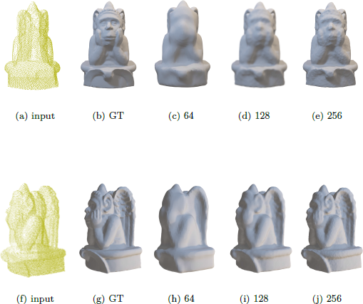
In Figures 5, 6, and 7, we show input point cloud scans, ground truth surfaces, and reconstructed surfaces using six methods - SPR+PCPNet, Points2Surf, Neural-Pull, POCO, NKSR, Geo-UDF, CAP-UDF, LevelsetUDF and LPSR (ours) for noise-free, original, and extra noisy categories, respectively. They are used for qualitative comparison of reconstructed surfaces under different settings. Besides, a visual illustration of different resolution outputs of LPSR are shown in Figure 8.
Generally speaking, LPSR produces accurate surfaces with no apparent failures. Although some details may be lost due to noisy inputs, no strange textures or artifacts exist in its reconstructed surfaces. In contrast, DL-based methods such as Neural-Pull and NKSR have partial failures, while Points2Surf exhibits unusual textures. Geo-UDF and CAP-UDF produce high-quality detailed geometry, though they struggle to maintain continuous surfaces in some local regions, resulting in broken pieces and non-manifold surfaces.
The success of LPSR is attributed to the PDE-based UDF decoder, which produces a smooth and monotonic UDF across most regions. In contrast, the DL-based models may decode surfaces from an ambiguous latent space, leading to unexpected local optima and, thus, unpredictable failures.
4.5 Ablation Study
In this section, we assess the effectiveness of each component using a subset of the ABC dataset.
1) Point Feature Projection. The number of projection directions in the point feature projection module significantly impacts model performance. We explored different configurations by varying the number of projection directions with m = 8,16, 24, 32, 64,128 and report the results in Table 8. We observed that the performance tends to drop with a smaller value m. This indicates that fewer projection directions limit the representation capability. When the number of projections is above 64, the performance saturates. Considering the complexity caused by larger feature dimensions, we selected m = 48.
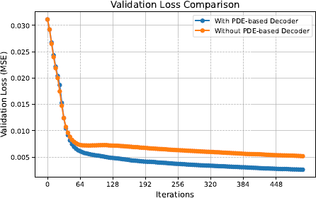
2) PDE-based decoder. We assess the effect of our PDE-based decoder by comparing our performance against a Sparse GUSL framework without a PDE-based decoder. The latter directly uses the unsigned distance value of each voxel as the prediction label.
Performance results are detailed in Table 9, showing a significant margin that validates the effectiveness of the PDE-based decoder. Additionally, we present the validation loss curves for the XGBoost model at the coarsest layer in Figure 9. The model without the PDE-based decoder exhibits early saturation, resulting in a higher loss. This performance gap stems primarily from the absence of the decoder, where XGBoost processes each voxel independently, disregarding the spatial correlations among neighboring voxels. In contrast, the PDE-based decoder captures the smoothness across the field, preventing the generation of discontinuous UDFs by the model.
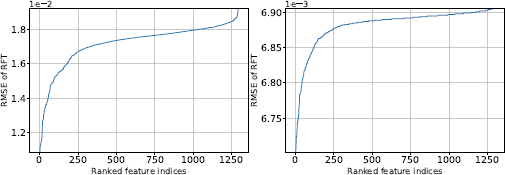
3) The Effect of Feature Selection. To achieve an optimal balance between low complexity and high performance, we investigated the impact of varying the number of features selected by our RFT module. We experimented with feature subsets of different sizes, selecting a subset of 32, 64, 128, 256, 512, 1024, and all generated features. The performance metrics for these configurations are detailed in Table 10. Our findings indicate that the RFT effectively maintains robust performance with as few as 256 selected features. Adding more features beyond this number results in performance saturation. This trend is also verified in Figure 10, where we plot the discriminative power of each feature at the coarsest and the second coarsest layers. Both figures illustrate that only a small percentage of the features have relatively strong discriminative power and majorly contribute to the model’s performance.
5 Conclusion and Future Work
A lightweight and interpretable surface reconstruction method, named LPSR, was proposed in this work. It offers high-quality reconstructed surfaces for various point cloud categories at lower computational and memory complexity. LPSR is mathematically transparent. It uses a feedforward-designed encoder and a PDE-based decoder, contributing to a deeper understanding of the surface reconstruction mechanism and model behaviors. The encoded representation has a clear physical meaning in controlling the surface shape, and it can be decoded at different grid resolutions to produce different levels of detail. The green learning paradigm further enhances the efficiency of LPSR. LPSR delivers high-quality reconstructed surfaces with a small feature dimension and minimal supervision.
We will extend LPSR to large-scale point cloud dataseis, such as indoor and outdoor scenes. We aim to understand the 3D shape generation behavior in these diverse contexts while maintaining mathematical transparency and computational efficiency.
The authors acknowledge the gift support from the Tencent Media Lab and the Center for Advanced Research Computing (CARC) at the University of Southern California for providing computing resources that have contributed to the research results reported in this publication. URL: https://carc.usc.edu.
![An illustration shows thirteen three D model renderings of a bone-like structure, labeled from a to m, where a is the Input point cloud, b is G T, and c through l are the results of different reconstruction methods, P G R [three three], G P S R [five nine], S P R plus P C P [one nine], P two S [one four], Neural-Pull [three], P O C O [five five], N K S R [two four], G e o hyphen U D F [four one], C A P hyphen U D F [five five], levelset U D F [five six], and m is Our L P S R.](https://emer.silverchair-cdn.com/emer/content_public/journal/atsip/14/2/10.1561_116.20240069/2/m_116.20240069005.png?Expires=1781775637&Signature=TDa3CjfP4rxZQzwJm6Hoebda-BjvmPGGvVXh5R4UNeeYi5Sh5epsfsTTJ9yFcDaDzRJtaAVS~Rbf1czZ0qfo9TYpOl3Ar91WS2GwGw1WOciRgTWLb6UtKf8jxGiPvlj9BPrIPhpXMt3yoVLGTKXjqa8vY5Qn45dVmSL-HBYVl3FGncxpoEnNUUPdAkQBmYBIa5IQzbwfCkTRuX28UkwMPH~Gkt2dbtIIZFotphhS3boxEGzUTaq-AsBfzGvpFslE7KSvGOC4LFGbmb70PLMA4nxTw6-YylyYjMUHCfGMXxFqxywa7CgYhhNVGOCbZUkwmoT5ycBGRJB5ivQGj7r-rw__&Key-Pair-Id=APKAIE5G5CRDK6RD3PGA)
![An illustration shows thirteen three D model renderings of a torus-like structure, labeled from a to m, where a is the Input point cloud, b is G T, and c through l are the results of different reconstruction methods, P G R [three three], G P S R [five nine], S P R plus P C P [one nine], P two S [one four], Neural-Pull [three], P O C O [five five], N K S R [two four], G e o hyphen U D F [four one], C A P hyphen U D F [five five], levelset U D F [five six], and m is Our L P S R.](https://emer.silverchair-cdn.com/emer/content_public/journal/atsip/14/2/10.1561_116.20240069/2/m_116.20240069006.png?Expires=1781775637&Signature=blCDB7lJF1LfvObtxrIamHKwMYIq5i8oHB~xVMPCCQRfVBANF4Rr0nsshmM54MTnkHxrNgJU2MTcpvCLwxXohZ26ONT3eJINpnUxjCIvv7P9GUN2teJSG5N6XXLNEIgS1kN6xOr960Qb9oYyypQ3uvHiR~ByWbuZ1jP2x7kqLIbLd~4nIM~wdskvrrXj-v4pnKus4GvZBs6iYWrF5MFEUccJGM~OIZu11bOTvCFqVeUEG1AcPnDRXdmQGFjypxJFEaQfHS0S~iWJo01jRyvv9u4HXX8x1tT3s4XGGgevIYLMtyfZYqz1EP7QsB9VPP-~WClNqA-jlW1aMdUaM4x4rg__&Key-Pair-Id=APKAIE5G5CRDK6RD3PGA)
![An illustration shows thirteen three D model renderings of a horse-like structure, labeled from a to m, where a is the Input point cloud, b is G T, and c through l are the results of different reconstruction methods, P G R [three three], G P S R [five nine], S P R plus P C P [one nine], P two S [one four], Neural-Pull [three], P O C O [five five], N K S R [two four], G e o hyphen U D F [four one], C A P hyphen U D F [five five], levelset U D F [five six], and m is Our L P S R.](https://emer.silverchair-cdn.com/emer/content_public/journal/atsip/14/2/10.1561_116.20240069/2/m_116.20240069007.png?Expires=1781775637&Signature=x1b0AgURbe6obPUYn3Y8UOJCVnJNvtuqCrB90nOSxbDcJj3fQaf5X6d-dfUub8ZWSbpRzrAMOjLAgGm6SA-GNIeRna5wVU6BXuTC6QT1rKysJZjsVK7mk~LaLoFsxhb6ZtiPtcC3EJljU7edux~Hm-OxLZIm020NYT87CnsHNrk2d0~6gcma4hV00zgd~lvrqRfsTg4koiXIt3JNF9IS4MEesbHYm5NeFoeXtFIQO-iuggCawIWYX901LI-YEX5Jejj~R2xd72UcpvHjStbA2IVT0QcNEuX7dfrQ2eZYvknyIgzU7MLDDGX4BhofvopKFdmD7X1nUQqgG4Oh1epDIg__&Key-Pair-Id=APKAIE5G5CRDK6RD3PGA)