


Moving object segmentation (MOS) is the process of identifying dynamic objects from video frames, such as moving vehicles or pedestrians, while discarding the background. It plays an essential role in many real-world applications such as autonomous driving, mobile robots, and surveillance systems. With the availability of a huge amount of data and the development of powerful computing infrastructure, deep learning-based methods have shown remarkable improvements in MOS tasks. However, as the dimension of data becomes higher and the network architecture becomes more complicated, deep learning-based MOS models are computationally intensive, which limits their deployment on resource-constrained devices and in delay-sensitive applications. Therefore, more research started to develop fast and lightweight models. This paper aims to provide a comprehensive review of deep learning-based MOS models, with a focus on efficient model design techniques. We summarize a variety of MOS datasets, and conduct a thorough review of segmentation accuracy metrics and model efficiency metrics. Most importantly, we compare the performance of efficient MOS models on popular datasets, identify competitive models and analyze their essential techniques. Finally, we point out existing challenges and present future research directions.
1 Introduction
Moving object segmentation (MOS) [59] is a fundamental task in computer vision. It is the process of extracting dynamic foreground content from video frames, such as moving vehicles or pedestrians, while discarding the non-moving background. MOS is used as a critical video pre-processing step followed by higher-level tasks such as traffic monitoring [39], target re-identification [251], action recognition [261], human detection [244], and object tracking [256]. However, with the increasing amount of produced visual data and computation-resource-limited platforms such as self-driving cars, wireless surveillance cameras, and navigation robots, it becomes quite crucial and challenging to process a large amount of video data in a timely fashion. In recent years, the research attention has moved toward developing more cost-efficient MOS models [36] by reducing the model size and computational complexity, increasing the inference speed, while achieving acceptable segmentation accuracy.
1.1 Background and Scope
In general, MOS tasks can be categorized as object-level segmentation and instance-level segmentation [69]. As illustrated in Figure 1(a), the goal of object-level segmentation is to detect all moving objects as the foreground and to generate a pixel-level binary segmentation mask, no matter the video scene has a single instance or multiple instances. For example, a horse and the person riding the horse are both detected as foreground, without being distinguished as two different instances. In contrast, as illustrated in Figure 1(b), instance-level segmentation not only detects the foreground moving objects, but also assigns each instance a different label, which can be utilized for object identification and tracking over time. For example, a man and two dogs are all detected as foreground, and these three instances are each assigned a different label. This shall be differentiated from video semantic segmentation (VSS), where instances having the same semantic meaning are assigned the same class label. In that case, the two dogs in Figure 1(b) will be assigned a single class label.
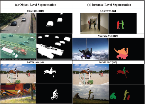
There are also several frequently used terms related to MOS: moving object detection (MOD), video object segmentation (VOS), and video salient object detection (VSOD). In the following, we will explain these terms, and define the discussion scope of MOS in this survey.
1.1.1 Moving Object Detection
Moving object detection (MOD) [6, 27, 91, 95, 169, 174, 235], also known as background subtraction [19, 59, 64, 89, 124, 180], is a traditional computer vision task that detects the changing foreground objects from static or dynamic background for video surveillance or anomaly detection purposes [59]. It can be viewed as an object-level segmentation task, which outputs a binary foreground mask without distinguishing different instances, as shown in Figure 1(a). Besides, dynamic elements in the background such as waving tree leaves, flowing water, snowing weather, are not the target objects to be detected.
1.1.2 Video Object Segmentation
In recent years, with the advances in deep learning and machine intelligence, the task of MOD is naturally extended to video object segmentation (VOS), to meet the requirement of emerging applications such as intelligence video editing, scene understanding, and autonomous driving. VOS refers to the task of segmenting main moving objects from a video sequence [165] which capture human attention. The early VOS task in the DAVIS 2016 challenge [164] is object-level segmentation, which only requires to segment one object or two spatially connected objects from a video sequence, generating a binary segmentation mask, as shown in Figure 1(a) DAVIS 2016 example. Later, multi-object VOS was introduced with the launch of the DAVIS 2017 challenge [165]. This task setting is more challenging as it is instance-level segmentation as shown in Figure 1(b), which requires not only separating the main moving objects from the background, but also discriminating different instances, generating a multi-class segmentation mask.
Depending on the level of human intervention during the segmentation process, VOS tasks can be divided into three categories: unsupervised VOS, semi-supervised VOS, and interactive VOS. In unsupervised VOS, human does not interact with the algorithm to obtain the segmentation results. In semi-supervised VOS [165], the algorithm is given a video sequence and the firstframe segmentation mask of the target objects, then the algorithm outputs the masks of those objects in remaining frames. Finally, interactive VOS assumes the user gives iterative refinement inputs to the algorithm, for example, in the form of a scribble, to segment the objects of interest. Methods have to produce a segmentation mask for that object in all the frames of a video sequence taking into account all the user interactions.
1.1.3 Video Salient Object Detection
A concept similar to unsupervised VOS is video salient object detection (VSOD) [67, 181]. VSOD aims also at finding objects in video frames that mostly attract human attention. However, it produces a sequence of probability maps that indicate the likelihood of each pixel belonging to most visually important objects. In contrast, unsupervised VOS outputs either a binary segmentation mask for single-instance case, or a multi-class segmentation mask for multi-instance case.
1.1.4 Moving Object Segmentation
In this survey, we mainly review state-of-the-art models for MOD, unsupervised VOS and semi-supervised VOS tasks. It is noteworthy that MOD can be considered as object-level unsupervised VOS. Since these three tasks all aim at segmenting main moving objects from videos, we adopt the term moving object segmentation (MOS), which differentiates our discussion scope from the original scope of VOS that also includes interactive VOS.
1.2 Overview of Existing MOS Approaches
Techniques used to segment video moving objects can be categorized as traditional approaches and deep learning-based approaches. Traditional approaches [11, 14, 15, 20, 28, 29, 39, 53, 68, 70, 72, 84−86, 117, 131, 145, 182, 185, 208, 211, 255, 256, 259, 262] do not require ground-truth labels for algorithm development. They usually include two components: background modeling and pixel classification. However, traditional methods meet difficulties when they are applied to complex scenarios, such as videos with dynamic backgrounds, shadows, illumination changes, and night scenes.
With the development of powerful computing infrastructure and the availability of a huge amount of data, deep neural networks (DNNs) have shown remarkable success in MOS tasks. Existing DNN-based MOS models are mostly supervised approaches based on 2D convolutional neural networks (CNNs) [8, 21, 35, 41, 42, 79−81, 96, 107−110, 133, 142, 160, 161, 172, 193, 194, 216, 248, 249], 3D CNNs [2, 58, 78, 127, 128, 171, 217], or generative adversarial networks (GANs) [9, 10, 158, 159, 186, 253, 254]. They demonstrated that DNNs can automatically extract spatial low-, mid-, and high-level features as well as temporal features, which turn out to be very helpful in MOS problems. Some methods combine both traditional methods and deep learning methods to get better performance such as RT-SBS [43], GraphMOS [63], and MotionRec [129].
Besides, semi-supervised video object segmentation (VOS) has emer-ged in recent years, in which the ground-truth segmentation mask of the first frame is provided during test time. This type of approach can be further categorized as (1) online fine-tuning-based methods, such as Meta-Learning [224], e-OSVOS [137], PreMOVS [123], etc.; (2) propagation-based methods, such as CTN [82], MaskTrack [163], FAVOS [37], AGSS [112], AGAME [88], DTN [245], SAT [32], Fasttmu [188], AOT-T [232], etc.; and (3) template-based methods, such as SwiftNet [206], STM [151], PLM [237], RANet [219], FRTM [170], TVOS [247], TTVOS [154], GC [105], LWL [13], MSN [222], RMNet [225], SiamMask [210], DDEAL [236], PiWiVOS [152], etc. The difference is that methods in category (1) need to re-train or fine-tune models online during the inference stage, and methods in categories (2) and (3) are usually used together and they do not need online model fine-tuning.
While existing DNN models provide superior MOS accuracy, they suffer from computationally expensive and memory-intensive problems. As the depth of neural network increases, the model size and computational complexity dramatically increase, making it challenging to apply these models to real-world scenarios, such as self-driving cars, robotics, and augmented reality. These tasks are typically deployed on mobile and embedded devices with limited memory and computing resources. Besides, they are usually latency-sensitive and need to be executed in a timely manner. High-complexity deep learning models cannot meet these requirements. Therefore, the research community now focuses more on designing cost-efficient deep MOS networks which have smaller model size, can achieve a faster inference speed, while maintaining high segmentation accuracy, so that they are suitable for mobile and embedded environments.
In this survey paper, we review the most recent advances in deep learning-based MOS techniques. We focus on fast and lightweight models and their performance on most popular MOS datasets. Besides, we provide a comprehensive list of existing MOS datasets and summarize performance evaluation metrics from both model accuracy and efficiency perspectives.
1.3 Previous Surveys
Table 1 lists existing surveys [6, 18, 19, 27, 59, 64, 89, 91, 95, 124, 132, 169, 174, 180, 213, 220, 234, 235] on MOS. Six of them [19, 27, 64, 132, 213, 234] reviewed recent deep learning-based MOS methods, and all the other surveys only focused on traditional methods.
Some surveys on deep learning-based MOS [19, 64] reviewed network architectures from background generation and background subtraction perspectives, and provided visual and quantitative performance evaluation on the CDnet 2014 dataset [215]. Methods about moving objects detection with a moving camera were also discussed [27], where a small number of deep learning models were briefly introduced. In [132], a detailed review of deep learning-based MOS model designs and evaluation settings is provided, such as different ways of splitting the training and test sets. It also provided performance evaluation on the CDnet 2014 dataset.
However, none of the aforementioned survey papers discussed techniques for efficient MOS model design for resource-constrained edge devices or delay-sensitive applications. They did not investigate fast or lightweight models, and did not compare inference speeds among different models. Besides, they did not discuss the newest MOS models developed in 2022, neither did they provide experimental studies on the recent popular MOS datasets such as DAVIS 2016 [164], DAVIS 2017 [165], and YouTube-VOS [227]. Moreover, the performance evaluation metrics introduced in existing surveys are limited. Recently, a comprehensive review on video object segmentation (VOS) models was conducted [213], including VOS datasets and VOS-oriented performance evaluation metrics. Nevertheless, it did not discuss fast and lightweight models, therefore it cannot provide insights for designing efficient models. Another survey on VOS [234] provided very limited discussion on efficient model design techniques. Besides, it did not present experimental results, and there were no comparison studies and analysis of model performance.
The summary of previous reviews on MOS.
| No. | Year | Title | Category | Author | Venue |
|---|---|---|---|---|---|
| 1 | 2014 | Traditional and Recent Approaches in Background Modeling for Foreground Detection: An Overview [18] | Non-Deep Learning | Thierry Bouwmans | Compure Science Review |
| 2 | 2014 | A Comprehensive Review of Background Subtraction Algorithms Evaluated with Synthetic and Real Videos [180] | Non-Deep Learning | Andrews Sobrala, Antoine Vacavant | Computer Visoin Image Understanding |
| 3 | 2015 | Moving Object Detection: Review of Recent Research Trends [95] | Non-Deep Learning | Jaya S. Kulchandani, Kruti J. Dangarwala | International Conference on Pervasive Computing (ICPC) |
| 4 | 2015 | Review: Moving Object Detection Techniques [6] | Non-Deep Learning | Amandeep, Er. Monica Goyal | International Journal of Computer Science and Mobile Computing |
| 5 | 2017 | Review on Moving Object Detection in Video Surveillance [91] | Non-Deep Learning | Aqsa Khan, Nitin J. Janwe | International Journal of Advanced Research in Computer and Communication Engineering |
| 6 | 2018 | A Survey on Moving Object Detection and Tracking Based On Background Subtraction [174] | Non-Deep Learning | Rahul Sharma, Subham Gupta | The Oxford Journal of Intelligent Decision and Data Science |
| 7 | 2018 | New Trends on Moving Object Detection in Video Images Captured by a Moving Camera: A Survey [235] | Non-Deep Learning | Mehran Yazdi, Thierry Bouwmans | Computer Science Review |
| 8 | 2019 | A Review on Moving Object Detection and Tracking Methods in Video [220] | Non-Deep Learning | Sarika S. Wangulkar, Roshani Talmale, Rajesh Babu | International Journal of Scientific Research in Science, Engineering and Technology IJSRSET |
| 9 | 2019 | Moving Object Detection Under Sudden Change of Illumination: A Review [169] | Non-Deep Learning | Rajib Debnath, Mrinal Kanti Bhowmik | International Journal of Computational Intelligence & IoT |
| 10 | 2019 | Background Subtraction for Moving Object Detection in RGBD data: A Survey [124] | Non-Deep Learning | Lucia Maddalena, Alfredo Petrosino | Journal of Imaging |
| 11 | 2019 | A Comprehensive Survey of Video Datasets for Background Subtraction [89] | Non-Deep Learning | Rudrika Kalsotra, Sakshi Arora | IEEE Access |
| 12 | 2019 | Background Subtraction in Real Applications: Challenges, Current Models and Future Directions [59] | Non-Deep Learning | Belmar Garcia-Garcia, Thierry Bouwmans, Alberto JorgeRosales Silva | Computer Science Review |
| 13 | 2019 | Deep Neural Network Concepts for Background Subtraction: A Systematic Review and Comparative Evaluation [19] | Deep Learning | Thierry Bouwmans, Sajid Javed, Maryam Sultana, Soon Ki Jung | Neural Networks |
| 14 | 2020 | Moving Objects Detection with a Moving Camera: A Comprehensive Review [27] | Deep Learning | Marie-Neige Chapel, Thierry Bouwmans | Computer Science Review |
| 15 | 2020 | Deep Learning Based Background Subtraction: A Systematic Survey [64] | Deep Learning | Jhony H. Giraldo, Huu Ton Le, Thierry Bouwmans | Handbook of Pattern Recognition and Computer Vision |
| 16 | 2020 | Video Object Segmentation and Tracking: A Survey [234] | Deep Learning | Rui Yao, Guosheng Lin, Shixiong Xia, Jiaqi Zhao, Yong Zhou | ACM Trans. Intell. Syst. Technol |
| 17 | 2021 | An Empirical Review of Deep Learning Frameworks for Change Detection: Model Design, Experimental Frameworks, Challenges and Research Needs [132] | Deep Learning | Murari Mandai, Santosh Kumar Vip parthi | IEEE Transactions on Intelligent Transportation Systems |
| 18 | 2021 | A Survey on Deep Learning Technique for Video Segmentation [213] | Deep Learning | Wenguan Wang, Tianfei Zhou, Fatih Porikli, David Crandall, Luc Van Gool | IEEE Transactions on Pattern Analysis and Machine Intelligence |
| 19 | Ours | A Survey of Efficient Deep Learning Models for Moving Object Segmentation | Deep Learning | - | - |
1.4 Our Contributions
In this work, we systematically review the most recent advances in deep learning-based MOS, with a focus on efficient (fast and lightweight) MOS models. Our major contributions are the following:
For the first time in the literature, we provide a comprehensive review of efficient MOS model design techniques which play an important role in mobile and embedded device applications and in delay-sensitive scenarios.
We discuss existing MOS datasets from the perspective of scene categories. We not only cover traditional MOD datasets such as CDnet 2014 and BMC [201] datasets, but also extend our discussion to newer VOS datasets such as DAVIS 2016, DAVIS 2017, and YouTube-VOS, which were designed for more complex scenes and higher resolutions.
We conduct a thorough review of model performance evaluation metrics, including segmentation accuracy metrics for object-level and instance-level segmentation as well as for salient object segmentation, and model efficiency evaluation metrics such as inference speed, model size, trainable parameters, and computational complexity. In contrast, existing MOS survey papers only introduced a subset of them.
We evaluate the performance of efficient MOS models on four most popular datasets: CDnet 2014, DAVIS 2016, DAVIS 2017, and YouTube-VOS. We identify models that are competitive in segmentation accuracy and inference speeds on these datasets, and analyze the essential techniques of these models.
We identify existing challenges in MOS and provide insights into future research directions.
The remainder of the paper is organized as follows. In Section 2, we introduce existing MOS methods, with a brief overview of traditional approaches, and a more detailed discussion on deep learning-based approaches. In Section 3, we discuss efficient MOS model design techniques and summarize models that use these techniques. Section 4 introduces representative datasets for a variety of scene categories. Section 5 presents performance evaluation metrics including segmentation accuracy metrics and model efficiency metrics. In Section 6, we provide comparison studies of existing efficient MOS models for popular datasets. Section 7 analyzes existing challenges in MOS and presents future research directions. Section 8 concludes the paper.
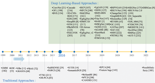
The timeline of MOS including traditional approaches [11, 14, 20, 28, 29, 53, 68, 72, 84–86, 131, 145, 182, 185, 208, 211] and deep learning approaches [3, 8, 9, 21, 32, 43, 63, 74–76, 78, 88, 96, 105, 109, 110, 112, 123, 127, 129, 133, 134, 141, 142, 147, 151, 152, 159–161, 170, 171, 175, 187, 193, 194, 198, 203, 206, 207, 210, 216, 217, 222, 225, 232, 240, 254].
The timeline of MOS including traditional approaches [11, 14, 20, 28, 29, 53, 68, 72, 84–86, 131, 145, 182, 185, 208, 211] and deep learning approaches [3, 8, 9, 21, 32, 43, 63, 74–76, 78, 88, 96, 105, 109, 110, 112, 123, 127, 129, 133, 134, 141, 142, 147, 151, 152, 159–161, 170, 171, 175, 187, 193, 194, 198, 203, 206, 207, 210, 216, 217, 222, 225, 232, 240, 254].
2 Existing MOS Approaches
MOS approaches can be categorized into traditional approaches and deep learning-based approaches. The chronological advancement in algorithms is depicted in Figure 2. Deep learning-based approaches are increasingly developed from 2016 and traditional approaches started in early 1999 and now are still being developed in parallel with deep learning-based approaches, and are even combined with deep learning approaches in a hybrid mode.
2.1 Traditional Approaches
Traditional approaches [11, 14, 15, 20, 28, 29, 39, 53, 68, 72, 84–86, 117, 131, 145, 182, 185, 208, 211, 255, 256, 262] do not require labeled ground-truth segmentation masks. They include two steps: background modeling and pixel classification. First, the background scene is initialized and updated over time, then each pixel is classified as foreground or background based on a threshold. Background modeling schemes can be parametric or non-parametric. Parametric approaches represent the background statistically using a probability density function (PDF) such as a single Gaussian or a mixture of Gaussians (GMM) [182, 262], and require to learn the parameters of these pdfs. Non-parametric approaches do not need to learn the parameters of probability distributions such as the kernel density estimation (KDE) method [53], or they do not have distribution assumptions for the background. There are also several sub-categories under the non-parametric approaches: filter-based, sample consensus, and principal-component-analysis (PCA) [116–118] methods. Examples of filter-based approaches are Kalman filtering [39], temporal median filtering [256], and running average filtering [255]. Examples of sample consensus methods are WeSamBE [86], ViBe [11], SuBSENSE [29], and PAWCS [28]. For instance, SuBSENSE uses a feedback system to adjust the background model automatically based on local binary similarity pattern (LBSP) features and pixel intensities [15]. PCA methods use eigenvalue decomposition for background modeling. To solve the camera motion problem, background subtraction based on robust principal-component analysis (RPCA) [84, 85] was also developed.
2.2 Deep Learning-Based Approaches
2.2.1 2D-CNN-based
Deep learning-based approaches have been recently proposed for MOS problems. The first deep learning-based work is ConvNet-GT [21] as shown in Figure 3(a), which performs change detection by replacing the pixel classification component with a well-defined neural network structure. The background is estimated with a temporal median filter, then it is stacked together with the original video frames to form the input of the CNN that outputs the binary masks. In a more advanced model MSFgNet [160], a motion-saliency network (MSNet) is used to estimate the background, which is then subtracted from the original frames, followed by a foreground extraction network (FgNet) that detects the moving objects. Another type of CNN is multi-scale feature learning-based CNN, which extracts multi-scale features to achieve better accuracy, such as MSCNN + Cascade [216], Guided Multi-Scale CNN [107], MCSCNN [108], MsEDNet [161] and VGG-16 [177] based networks FgSegNet_M [96] and FgSegNet_v2 [110]. In MSCNN+Cascade [216], segmentation results are generated pixel by pixel. Although it achieves good accuracy, the pixel-wise processing is very time consuming. In FgSegNet_M [96] as shown in Figure 3(b), a 2D CNN takes each video frame at three different resolution scales in parallel as the input of the encoding network.
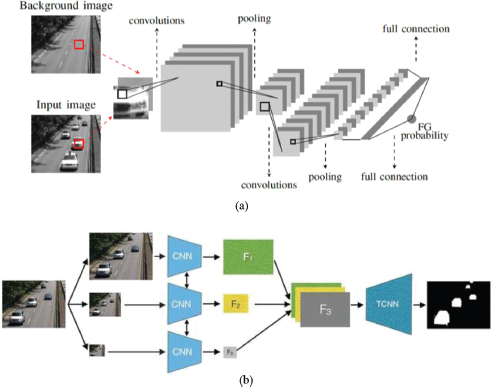
2D-CNN-based models: (a) ConvNet-GT (Copyright © 2016 IEEE [21]), (b) FgSegNet_M (Copyright © 2018 Elsevier B.V. [96]).
2.2.2 3D-CNN-based
The advantage of 3D convolution for MOS problems is that 3D convolution can utilize spatial-temporal information in visual data, which helps improve model accuracy. For example, in 3D CNN-LSTM [2] as shown in Figure 4(a), short-term temporal motions of a video sequence are captured by 3D convolutions, while the long-short term temporal motions are captured by 2D LSTM modules. Another example is 3DAtrous [78], which also captures long-term temporal information in the video data. It is trained based on an LSTM network with focal loss to tackle the class imbalance problem commonly seen in background subtraction. Besides, 3D-CNN-BGS [171] utilizes 3D convolution to track temporal changes in video sequences. It performs 3D convolution on 10 consecutive frames of the video, and upsamples the low-, mid-, and high-level feature layers of the network in a multi-scale approach to enhance segmentation accuracy. In [58], 3D CNN and a fully connected layer are adopted in a patch-wise method. In 3DS_MM [75] as shown in Figure 4(b), 3D separable convolutional neural network with a multi-input multi-output strategy is proposed, in which the standard 3D convolution is decomposed into depthwise and pointwise convolutions, in order to reduce model size and computational complexity.
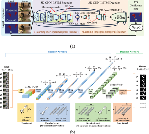
3D-CNN-based models: (a) 3D CNN-LSTM model (Copyright © 2020 IEEE [2]), (b) 3DS_MM [75] model using 3D separable CNN.
2.2.3 GAN-based
Generative adversarial networks (GAN) is also adopted in MOS problems. BScGAN [10] as shown in Figure 5(a) is based on conditional GAN (cGAN), in which the discriminator not only takes the foreground mask as the input, but also takes the stacked color image and its background as a conditional input to improve segmentation accuracy. FgGAN [159] shown in Figure 5(b) adopted GAN-based unpaired learning to solve challenging MOS problems such as dynamic background, bad weather, effect of shadow and irregular motion of objects. Since the training set has unpaired input and output images, this network is trained by adding a cycle-consistent loss in the traditional GAN loss. First, a video-wise background is estimated using GAN-based unpaired learning network (network-I). Then, to extract the motion information related to foreground, motion saliency is estimated using the estimated background and current video frame.
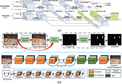
Further, the estimated motion saliency is given as the input to another GAN-based unpaired learning network (network-II) for foreground segmentation. In BSPVGAN [254], a median filter was used for background modeling and Bayesian GANs were adopted for pixel classification, because Bayesian GANs can address the problem of ghost, non-stationary background, and sudden illumination changes. Meanwhile, BSlsGAN [186] utilized conditional least squares adversarial networks, in which the generator loss function includes the Lı-loss and perceptual-loss between the generated segmentation mask and its respective ground truth to learn dynamic background variations. DBSGen [9] was also developed to address the dynamic background subtraction problem, which used two generative neural networks, one for dynamic motion removal and the other for background generation. The networks were optimized in an end-to-end fashion. Finally, the foreground moving objects were obtained by a pixel-wise distance threshold based on a dynamic entropy map.
2.2.4 Unsupervised VOS
Unsupervised video object segmentation (UVOS), also known as zero-shot VOS, automatically segments and tracks primary moving objects in a video sequence without any prior information. Early UVOS in DAVIS 2016 Challenge is object-level segmentation which generates binary segmentation masks and is relatively simple [51, 67, 104, 181, 195]. Besides, MOD tasks can also be considered as object-level unsupervised VOS.
With the launch of DAVIS 2019 Challenge, multi-object UVOS has become a hot topic. This task is more challenging as it is instance-level segmentation, which requires automatically discriminating different object instances and associating the same identities over time. An early approach RVOS [202] incorporated recurrent layers spatially and temporally to discover different object instances within a frame, and to keep the coherence of segmented objects along time. Since the network shared the encoder forward pass for all the objects in a frame, it achieved a fast overall runtime, although the segmentation accuracy is relatively low. More sophisticated models followed a two-stage paradigm: (1) detect object proposals using pre-trained Mask R-CNN, and (2) conduct generic feature matching for temporal association using re-identification techniques [212, 257, 263]. Although these approaches achieved higher accuracy, they are computationally expensive. For example, UnOVOST [263] not only requires Mask R-CNN for instance proposal generation, but also needs to compute optical flow for motion estimation. Complex post-processing and heuristics also make this method unsuitable for practical applications.
Recently, to strike a better balance between accuracy and efficiency, the model in [258] formulates instance proposal and foreground estimation in a unified framework, requiring much less time to generate instance proposals than Mask R-CNN based methods. Besides, it does not require additional post-processing components.
2.2.5 Semi-Supervised VOS
Semi-supervised VOS, also known as one-shot VOS, has emerged with the launch of DAVIS 2017 Challenge [165]. It incorporates human intervention during the inference stage. The most typical human intervention is to provide the ground-truth object mask of the first frame of the video. Many semi-supervised VOS models are trained and evaluated on the DAVIS 2016 dataset [164] designed for object-level segmentation, or on the DAVIS 2017 [165] and YouTube-VOS [227] datasets designed for instance-level segmentation.
Deep learning models for semi-supervised VOS tasks can be categorized as online fine-tuning-based, template-based, and propagation-based methods. Online fine-tuning-based methods first learn general segmentation features offline from images and video sequences, then fine-tune the model at test time with the ground-truth object mask of the first frame. For example, PReMVOS [123] adopts online fine-tuning, which first generates a set of object segmentation mask proposals for each video frame, followed by selecting and merging these proposals into accurate and temporally consistent pixel-wise object tracks over a video sequence. It won both the 2018 DAVIS Challenge on VOS and the 2018 YouTube-VOS challenge.
On the other hand, template-based methods use the first frame with its ground-truth mask to extract object features as a template, then segment objects from subsequent frames by matching their features with the template. Examples of template-based methods are RANet [219] and TTVOS [154]. RANet applies a ranking system to the matching process between multiple templates and the input to extract reliable results. TTVOS combines short-term matching and long-term matching, in which short-term matching enhances target object localization and long-term matching improves fine details and handles object shape-changing. Propagation-based methods use the previous frame mask to infer the current frame mask. One example is MaskTrack [163], which proceeds on a per-frame basis, guided by the output of the previous frame towards the object of interest in the next frame.
2.2.6 Other Approaches
Some foreground and background segmentation models use data augmentation techniques to improve the performance of prior models. For example, data augmentation performed in [172] not only creates endless data on the fly, but also features semantic transformations of illumination, which enhances the generalization capability of the model. It successfully simulates flashes and shadows by applying the Euclidean distance transform over a randomly generated binary mask. Such data augmentation allows to effectively train an illumination-invariant deep learning model for background subtraction. Another example using data augmentation is [93]. Two data augmentation methods of adjusting background model images and past images are proposed and applied to their previously proposed foreground segmentation framework [92]. Through this method, the segmentation performance is improved in difficult areas such as static foreground and ghost objects, compared to previous studies.
3 Efficient MOS Model Design
Although deep learning-based MOS models have achieved high accuracy in recent years, they come at a high computational cost and a slow inference speed due to complex network structures and intense convolution operations. The need for efficient models that require less inference time is vital, especially for applications such as autonomous driving. In the following, we summarize techniques used to design efficient deep neural network architectures to reduce the inference time, computational complexity and model size, while maintaining high segmentation accuracy. Existing models using these techniques are summarized in Table 2.
3.1 Asymmetric Convolution
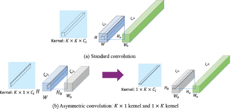
Asymmetric convolution is to factorize a standard two-dimensional convolution kernel into two one-dimensional convolution kernels. As shown in Figure 6, a K × K convolution can be substituted with a K × 1 convolution followed by a 1 × K convolution. Such a scheme can effectively reduce network parameters and required calculations. For example, when the input channel Ci is the same as the output channel Co, the number of parameters and computational cost are saved by 33% for a 3 × 3 kernel [189], and the performance degradation is often very small. A real-time foreground segmentation model DRSNet [205] uses asymmetric convolutions in its proposed MultiScaleSE Block, DoubleConv Block and NeckConv Block, to replace symmetric convolutions to reduce parameters and to ensure segmentation accuracy at the same time.
Efficient MOS model design techniques.
| Efficient Model Design Techniques | MOS Models | ||
|---|---|---|---|
| 3.1 | Asymmetric Convolution | DRSNet [205] | |
| 3.2 | Dilated Convolution | DRSNet[205]; A Past X-shaped with CompactASPP [241]; One-Shot Animal [228]; U2- ONet [204]; Frame-Level Weakly Supervised [139]; Espnet [135]; PDB [181]; PyramidCSA [67] | |
| 3.3 | Group Convolution and Depth-Wise Convolution | 2D _ Separable CNN [74]; One-Shot Animal [228]; 3DS _ MM [75]; F3DsCNN [76] | |
| 3.4 | Reduce Feature Map’s Volume | ChangeDet [133]; 3DPR [127]; U2-ONet [204]; AOT-T [232]; PRTM-fast [170]; FRTM [170]; G-PRTM-fast [155]; SiamMask [210]; DRSNet [205]; Adaptive Template [156]; MFCN [240] | |
| 3.5 | Simplified Network Architecture | MSFgNet [160]; AGSS [112]; One-Shot Animal [228]; PiWiVOS-F [152]; FCESNet [168]; PAMINet [120]; Lightweight U-Net-like [111]; Guided Multi-Scale CNN [107]; MSCNN + Cascade [216]; Trip-Net [147] | |
| 3.6 | Two-Branch Network | F3DsCNN [76]; ContextNet [166] | |
| 3.7 | Channel Merging by Addition | DRSNet [205]; Lightweight U-Net-like [111] | |
| 3.8 | Decoder Size Reduction | One-Shot Animal [228]; 2D _ Separable CNN [74]; 3DS _ MM [75]; F3DsCNN [76] | |
| 3.9 | Quantization | T-RexNet [24]; S3-Net [38] | |
| 3.10 | Small Convolution Kernel | A Past X-Shaped with CompactASPP [241]; Frame-Level Weakly Supervised [139]; MSFgNet [160] | |
| 3.11 | Skip Connection | Lightweight U-Net-like [111]; BMN-BSN [142]; BSUV-Net 2.0 [193]; 3D CNN-LSTM [2]; BScGAN [10]; U2-ONet [204]; Edge Aggregation Network [157]; LSTNet [207]; Frame-Level Weakly Supervised [139]; MvRF [3] | |
| 3.12.1 | Improving the Efficiency of Semi-Supervised VOS | Meta Learning | Meta-Learning [224]; e-OSVOS [137] |
| 3.12.2 | Template-Based and Propagation-Based Methods | SAT-Fast [32]; SAT [32]; Fasttmu [188]; SwiftNet [206]; RANet [219]; FRTM-fast [170]; | |
| FRTM [170]; G-FRTM-fast [155]; TVOS [247]; TTVOS(HRNet) [154]; TTVOS(ResNet5O) [154]; GC [105]; LWL [13]; MSN [222]; RMNet [225]; SiamMask [210]; | |||
| DDEAL(Res101) [236]; LSTNet [207]; Adaptive Template [156]; AGSS [112] | |||
| 3.13 | Multi-Input Multi-Output Strategy | 3DS _ MM [75]; F3DsCNN [76]; FCESNet [168] | |
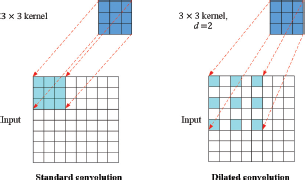
An illustration of the dilated convolution with kernel size k = 3 and dilation rate d =2. Both the standard convolution and dilated convolution have the same number of parameters (i.e. kernel size is 3 × 3), whereas the dilated convolution has a larger 5 × 5 receptive field.
An illustration of the dilated convolution with kernel size k = 3 and dilation rate d =2. Both the standard convolution and dilated convolution have the same number of parameters (i.e. kernel size is 3 × 3), whereas the dilated convolution has a larger 5 × 5 receptive field.
3.2 Dilated Convolution
Dilated convolution is adopted in MOS [204, 205, 228, 241] to allow larger receptive field with the same computation and number of model parameters (weights). In [228], dilated convolutions are implemented with different dilation rates to increase the receptive field for video segmentation. As illustrated in Figure 7, for a k × k dilated convolutional kernel with a dilation rate of d > 1, the effective size of the kernel is increased to [(k − 1)d +1]2. However, only k × k pixels participate in the convolutional operation, reducing the computational cost while increasing the effective kernel size and receptive field [135].
It is worth noting that dilated convolution is usually combined with multi-scale schemes to extract features. In PDB [181], multi-scale features are extracted by dilated convolution with different dilation rates to generate features with different receptive fields, which reduces complexity compared to using large kernel sizes. In PyramidCSA [67], multi-scale features are extracted by constrained self-attention with different attention window sizes and dilations in parallel branches, to capture motion cues of multi-scale objects and objects moving at various speeds. It has much less computation and memory usage than the non-local attention mechanism which extracts global context.
3.3 Group Convolution and Depth-Wise Convolution
To reduce computational cost and model size, group convolution is adopted in [156]. The idea of group convolution was first introduced in AlexNet [94] to use the limited memory of two GPUs to train the model in parallel. Since then, it has been widely applied in computation-efficient network architecture designs. As shown in Figure 8, a group convolution splits the channels of the input feature maps into G mutually exclusive groups, then convolution is independently performed on each group, followed by output channel concatenation. Theoretically, it can reduce both the computational complexity and model parameters by a factor of G.
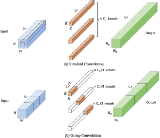
An illustration of the group convolution with three groups G = 3. Each group of input is convolved with (Co/3) kernels of size K × K × (Ci/3), to generate an output of size Ho× Wo× (Co/3). Three groups of outputs are concatenated to form the final result.
An illustration of the group convolution with three groups G = 3. Each group of input is convolved with (Co/3) kernels of size K × K × (Ci/3), to generate an output of size Ho× Wo× (Co/3). Three groups of outputs are concatenated to form the final result.
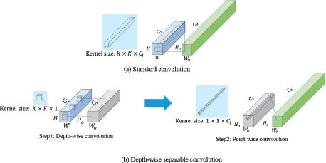
The method of depth-wise convolution was first proposed in MobileNet [77]. As demonstrated in Figure 9, it decomposes a standard 2D convolution into a depth-wise convolution (also known as spatial or channel-wise convolution) and a 1 × 1 point-wise convolution. While the depth-wise convolution applies an independent 2D filter for each input channel, the subsequent point-wise convolution performs 1D convolutions on the output of the depth-wise convolution along the channel direction. This separation can effectively reduce the amount of computation and model size. For example, when the filter size is K × K, the computational cost of 2D separable convolution can be reduced to roughly of that of the standard 2D convolution. It can dramatically increase the inference speed while maintaining high detection accuracy. This idea was utilized in 2D_Separable CNN [74] and One-Shot Animal model [228] for video moving object segmentation.
To further exploit the temporal information in the video input, the 3DS_MM model was proposed [75], which adopts 3D convolution to extract spatiotemporal features in the video data and to improve segmentation accuracy. To reduce computational complexity and model size, the standard 3D convolution is decomposed into a depth-wise convolution and a point-wise convolution. While the depth-wise convolution performs a spatial-temporal convolution independently on each input channel, the subsequent point-wise convolution along the channel direction can effectively leverage channel correlations. When K × K × K is the spatial-temporal filter size, the computational cost of such a 3D separable convolution can be reduced roughly to of that of the standard 3D convolution.
On the other hand, since it is better to apply nonlinear activations in a high-dimensional space than in a low-dimensional space to prevent information loss, MobileNetV2 [173] introduces the inverted residual bottleneck module. The input features with Cl channels are first expanded to a high-dimensional space with Ch > Cl channels using a point-wise convolution. Subsequently, a 2D depth-wise convolution with nonlinear activations is performed on each of these Ch channels. Afterwards, another point-wise convolution with linear activatons projects the features back onto a low-dimensional space with Cl channels. To utilize spatio-temporal information in video data and to increase segmentation accuracy, the method proposed in F3DsCNN [76] replaces such 2D separable convolutions in the inverted residual bottleneck by 3D separable convolutions.
3.4 Reduce Feature Map’s Volume
Convolution-based feature extraction has high computational complexity due to large image resolution and large number of channels. Methods are typically used in MOS to reduce the volume of feature maps. In particular, large-scale down-sampling can be used to reduce the input image (or feature map) resolution before applying more convolutional layers, and point-wise convolution can be used to reduce the number of channels. Such techniques can be found in [127, 133, 155, 156, 170, 204, 205, 210, 232, 240]. For example, in U2-ONet [204], OctConv (Octave Convolution) [34] is used to reduce spatial redundancy. It is well-known that natural images can be decomposed into a low and a high spatial frequency part. While the low-frequency part represents global structures, the high-frequency part contains fine details. Similarly, the feature maps of a convolution layer can also be factorized to low-frequency and high-frequency components. OctConv stores and processes the smoothly changing, low-frequency feature maps in a low-resolution tensor to reduce spatial redundancy, meanwhile reducing the memory and computation cost. Another example is a shallower network ChangeDet [133] which utilizes fewer number of kernels to reduce feature map channels, and uses max pooling to reduce feature map resolutions. This results in only 0.13 millions of trainable parameters with a model size of only 1.6 megabytes (MB).
3.5 Simplified Network Architecture
To reduce model size and computational cost, simplified network architectures are also used in MOS models. In FCESNet [168], there is no fully connected layers, and the network only contains 7 layers, which reduces the number of parameters and increases the inference speed. FAMINet [120] is proposed to include feature extractor, appearance network, motion network and integration network. The appearance network generates an initial segmentation, the motion network generates an optical flow, then the integration network takes these results and previous frames’ predictions as its inputs, and outputs the final refined segmentation result. For efficiency, the motion network only has two convolutional layers and the integration network only has five convolutional layers. In the Lightweight U-Net-like model [111], thinner convolution layers are utilized to achieve an inference speed of 250 frames per second (fps) on a GTX Titan Xp GPU. The model size is only 435 kilobytes (KB). There are only 0.105 millions of model parameters, and only 0.13 billion floatingpoint operations (GFLOPs) are needed. In the One-Shot Animal Model [228], the proposed encoder module Xception-lite for video object segmentation is inspired by Xception-65 backbone [40]. While the original Xception-65 backbone has 65 layers to extract visual features which is time-consuming, the Xception-lite model only has 20 layers. To achieve the best trade-off between accuracy and speed, Xception-lite also incorporates residual connections and separable convolutions. Such simplified network architectures can also be found in Guided Multi-Scale CNN [107], MSCNN+Cascade [216], MSFgNet [160], Trip-Net [147], PiWiVOS-F [152], etc.
3.6 Two-Branch Network
Segmenting high-resolution inputs directly with classical frameworks like fully convolutional networks (FCN) [121] is time consuming. To overcome this shortcoming, the two-branch network scheme was proposed. The network consists of two branches, while one branch is shallow, captures spatial details and generates high-resolution feature representation, the other branch is deep and obtains high-level semantic context. Finally, the two-branch output feature maps are fused to generate the segmentation result. For example, ContextNet [166] as shown in Figure 10(a) processes the video frame at two resolutions in two parallel branches for semantic segmentation. In F3DsCNN [76] as shown in Figure 10(b), the 3D convolution-based two-branch scheme is adopted to extract spatial-temporal information for video moving object segmentation. Moreover, F3DsCNN proposed to share the first few layers of the two branches such that the model size and complexity can be further reduced. Similar ideas were also adopted in ICNet [250] and FgSegNet_v2 [110], which extended the two-branch network to three-branch networks to extract low-, mid-, and high-level features.
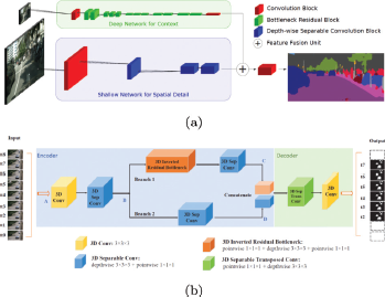
Using such two-branch or multi-branch networks can get high quality segmentation results, since the high-resolution branch helps recover and refine the coarse prediction produced by the low-resolution branch. Although some details are missing and blurry boundaries are generated in the low-resolution branch, it already harvests most semantic parts.
3.7 Channel Merging by Addition
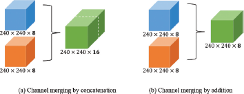
To integrate shallow and deep semantic layers, usually channel concatenation is used as in Figure 11(a). However, it increases the computational cost of subsequent convolution layers since the number of channels increases. As illustrated in Figure 11(b), to reduce the computational cost, addition can be used to merge channels [205], [111]. In particular, the Lightweight U-Net-like model [111] adopts element-wise summing for feature fusion in the decoder, which stabilizes training convergence, and also achieves an inference speed of 250 fps on an Nvidia GTX Titan Xp GPU with a model size of 435 KB and 0.105 millions of trainable parameters.
3.8 Decoder Size Reduction
The encoder-decoder network is one of the most standard architectures of object segmentation. It is suggested that the architecture of an encoder-decoder model can be simplified by reducing the decoder’s size, in order to save computational cost. In other words, we can adopt an asymmetric encoder-decoder architecture in which the encoder is larger than the decoder, instead of a symmetric encoderdecoder architecture. The rationale behind this idea is that the encoder should work in a similar fashion to original classification architectures, which extract deep features of smaller resolutions. On the contrary, the role of the decoder is to up-sample the output of the encoder, only enhancing its details. Therefore, reducing the decoder’s size results in computational cost savings. Overall, this approach is appealing since most of the time the reduction in the decoder’s size does not affect segmentation accuracy.
Decoder size reduction has been demonstrated in [74] and [75], in which the number of decoder layers is less than that of the encoder layers, which achieves faster inference speed without affecting the accuracy. In F3DsCNN [76], the last deconvolution layer in the decoder is replaced by upsampling to further increase the inference speed. In the One-Shot Animal model [228], the encoder is a deep network that generates five stages of shallow to deep feature maps. The feature maps are then upsampled and concatenated to form the final encoded feature map. In contrast, the decoder simply performs a 1 × 1 convolution to linearly fuse these feature maps to output a 1D probability map as the segmentation result, followed by post-processing to fine-tune the segmentation accuracy.
3.9 Quantization
The runtime of a network can be further reduced using quantization techniques. These techniques reduce the size/memory requirements of a network by encoding parameters in low-bit representations. In [38], quantization is adopted in both training and inference with 8-bit weights and features, which results in significant model compression and efficiency enhancement. In [24], the experiments were conducted with the half-precision floating point (FP16) format since this provides a good trade-off between accuracy and power consumption. The use of FP16 has achieved a good frame rate on the NVIDIA Jetson Nano edge-device, which shows its suitability for real-time applications [24].
3.10 Small Convolution Kernel
To benefit from rich contextual dependencies, an MOS model can use standard convolutions with large kernel size to enlarge the receptive field. However, it is harmful to use excessively large kernels, because they might lead to over-fitting [162], and increase the model size and complexity, especially when they are used in deep layers with a large number of input feature map channels. To address this problem, in [241], small kernel size is adopted along with dilated convolution (atrous convolution), which effectively enlarges the receptive field to capture long-range dependencies, meanwhile avoiding problems that may be caused by large kernels.
Although large kernels were adopted in [115] and [47] to close the performance gap between CNNs and transformers [48, 119], it is noteworthy that these methods [47, 115] adopt large kernels in depth-wise convolution to control the computational complexity. In particular, [115] also utilized inverted bottleneck, such that the depth-wise convolution with a large kernel is performed when the feature channels are small, followed by 1 × 1 point-wise convolution which raised the channel to a higher-dimensional space.
3.11 Skip Connection
Skip connection (or shortcut connection) is a technique that has demonstrated its effectiveness in maintaining high segmentation accuracy without adding network complexity, and has been adopted in classic lightweight models such as MobileNetV2 [77] and SqueezeNet [61].
In the Lightweight U-Net-like MOS model [111] as shown in Figure 12, long and short skip connections are proposed to facilitate data flow and maximize the usage of parameters in the model, enabling a lightweight design and leading to faster networks. As shown in Figure 12(a), long skip connections ship low-level features extracted by the second encoder layer directly across networks and share them to the corresponding decoding layer. Since the texture details are captured by low-level features and are usually lost in deep layers, long skip connections can provide decoders with such low-level features to more effectively infer the foreground masks. Compared to multi-scale feature extraction [216], long skip connections make one pass sufficient to pass richer information to the other end of the network [111]. On the other hand, short skip connections are adopted in bottleneck blocks of the network to enhance feature utilization rate, such that the bottleneck blocks in [111] can be designed as compact as possible. Figure 12(b) shows the detailed structure of the bottleneck block, which consists of four mini-blocks. Each mini-block is an extremely lightweight operation block that further consists of one convolutional layer, one instance normalization, and one parametric ReLU layer. As shown in Table 4, such efficient design of the Lightweight U-Net-like model achieved the highest F-measure (97.7%) with the fastest inference speed (250 fps) and required the fewest model parameters (0.1 M) among all models under the Titan Xp GPU group.
Skip connection is also used in BMN-BSN [142], BSUV-Net2.0 [193], 3D CNN-LSTM [2], BScGAN [10], U2-ONet [204], Edge Aggregation Network [157], Long-Short Term Network (LSTNet) [207], Frame-Level Weakly Supervised Network [139], and MvRF-CNN [3] for MOS tasks. Besides, asymmetric skip connections [205] was also proposed, which can more effectively integrate information from different semantic layers than symmetric skip connections, while requiring smaller number of network parameters.
3.12 Improving the Efficiency of Semi-Supervised VOS
Recently, more and more semi-supervised VOS models (one-shot learning) have emerged, in which the object mask of the first frame is provided in the inference process, and the goal is to automatically segment the target object from the entire video sequence.
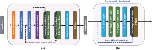
(a) Long and short skip connections in the Lightweight U-Net-like MOS model [111], and (b) the Asymmetric Bottleneck block of (a), using a short skip-connection.
(a) Long and short skip connections in the Lightweight U-Net-like MOS model [111], and (b) the Asymmetric Bottleneck block of (a), using a short skip-connection.
There are three types of one-shot learning for video object segmentation: online fine-tuning, template-based, and propagation-based. Online fine-tuning refers to approaches that fine-tune a general-purpose segmentation model on the annotated first frame during test time using hundreds of iterations of gradient descent [230]. Due to the heavy computation burden of fine-tuning, the processing speed of such methods cannot satisfy the requirements for practical applications. To alleviate the complexity issue of online fine-tuning, meta learning can be used to optimize the online fine-tuning process [137, 224]. Or, template-based and propagation-based methods can be used to refrain from online fine-tuning.
3.12.1 Meta Learning
Meta learning, also known as “learning to learn”, uses a bunch of similar learning tasks to train a meta-learner, such that it can adapt to a new task quickly with only a few training samples. In [224], a meta-learner is trained on multiple VOS tasks such that the meta model can capture their common knowledge and gains the ability to fast adapt the segmentation model to new video sequences. The e-OSVOS [137] approach meta learned the model initialization and learning rates for test time optimization by predicting individual learning rate at a neuron level. Furthermore, it applies an online adaptation to address the common performance degradation problem for future frames in the video sequence.
3.12.2 Template-Based and Propagation-Based Methods
In addition to meta learning, template-based and propagation-based methods (introduced in Section 2.2.5) are also proposed to alleviate the dependence on the online fine-tuning process, and they are usually combined in many fast VOS models.
However, template-based methods can suffer from memory issues because historical frames need to be memorized and updated, and propagation-based methods are vulnerable to temporal discontinuities like occlusions and rapid motion. To solve these problems, a real-time model SwiftNet [206] updates fewer frames in memory and adaptively selects incremental frames that have variations for memory update and ignores static ones. Besides, it abandons full-frame operations and incrementally processes with temporally varying pixels. Similarly, [156] adaptively updated the shape variation of target objects without heavy computation or additional memory. In [105], fixed-size feature representation is used to reduce memory which is needed in the template matching process. In the Regional Memory Network (RMNet) [225], local-to-local matching is performed between the current query frame and past frames. This effectively addresses the problems of mismatching to similar objects and high computational complexity caused by global-to-global matching. DDEAL [236] learns static cues from the labeled first frame and dynamically updates cues of subsequent frames for object segmentation. In [207], both template-based and propagation-based strategies were explored to match for pixel-level object segmentation and to handle the mismatching and drifting problem. In particular, the proposed long-term network exploits the object relationship between the current frame and the first frame, and the proposed short-term network explores immediate object variations.
3.13 Multi-Input Multi-Output Strategy
Another factor that affects the performance of a model is the input-output relationship. As shown in Figure 13, the input-output relationship of existing MOS networks has three types. The first type is single-input single-output (SISO), which is widely exploited in 2D CNNs such as FgSegNet_S [96] and 2D_Separable CNN [74]. The second type is multi-input single-output (MISO) which can be found in 3D CNNs such as 3D-CNN-BGS [171], 3DAtrous [78], and DMFC3D [217]. The disadvantage of SISO and MISO is that they result in a slow inference speed because only one frame output is predicted in every forward pass. The third type of input-output relation is multi-input multioutput (MIMO) such as FCESNet [168], which can take multiple input frames and output multiple frames of segmentation masks in each forward pass. It explores temporal correlations on a larger time span. Two recent models 3DS_MM [75] and F3DsCNN [76] combined the MIMO strategy with 3D separable CNN, which significantly increase the inference speed, so that they are suitable for computation-resource-limited and delay-sensitive applications.
3.14 Summary
Among the efficient techniques discussed above, the two-branch network [76, 166] and skip connection [111, 205] are very effective for scenarios such as MOS and semantic segmentation in which both high-level semantics and low-level details are needed. The two-branch network and skip connection extract high-level semantics by deep network layers to infer segmentation class labels, and extract low-level details by shallow network layers to recover segmentation boundaries. These two techniques also have the merit of reducing computational complexity, since only small-resolution features are processed by deep layers, while large-resolution features are processed by shallow layers. Besides, channel merging by addition can be used after these two schemes to reduce the feature volume and computation.
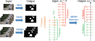
The input-output relationship of MOS models: single-input single-output (SISO), multi-input single-output (MISO), and multi-input multi-output (MIMO) [75].
The input-output relationship of MOS models: single-input single-output (SISO), multi-input single-output (MISO), and multi-input multi-output (MIMO) [75].
When the dilated convolution is combined with multi-scale processing, it is very effective for dense prediction tasks [190], such as MOS, semantic segmentation, super-resolution, and image denoising. The reason is that multi-scale dilated convolution with different dilation rates can extract features from small to large receptive fields to model both local and global patterns. Meanwhile, it avoids increasing the kernel size.
The multi-input multi-output (MIMO) strategy is very effective in increasing the inference speed for MOS [73, 75, 76] and other video-related tasks, such as video frame prediction. Since multiple video frames can share the intermediate layers of the network, the computational complexity can be effectively reduced. On the other hand, decoder size reduction [74–76, 228] is useful to reduce the complexity of segmentation networks such as those for MOS and semantic segmentation. In these networks, a deep encoder is needed to extract high-level semantic features from pixels, while the decoder can be shallow, which only needs to generate the segmentation mask without recovering texture details.
Other techniques such as asymmetric convolution, depth-wise convolution, group convolution, reduce feature map’s volume, simplified network architecture, quantization, and small convolution kernel can be used for not only MOS, but also general computer vision tasks, such as image classification and object detection. In particular, asymmetric convolution, depth-wise convolution, and group convolution are similar in the sense that they all decompose a standard convolution into several steps. Recent research [75, 76, 156, 205] shows that they effectively reduce model parameters (kernel weights) and computation for MOS tasks.
4 Datasets
Table 3 provides numerous existing datasets for the training and evaluation of MOS models [4, 12, 16, 17, 22, 23, 44–46, 52, 66, 87, 90, 97–101, 103, 125, 126, 129, 130, 138, 143, 149, 150, 164, 165, 167, 178, 179, 184, 192, 196, 197, 200, 201, 209, 214, 215, 223, 227, 233, 238]. Most of these datasets are for object-level segmentation, such as CDnet 2014 [215], DAVIS 2016 [164], UCSD [126], etc., hence the ground-truth masks contain binary labels. Some of the datasets are for instance-level segmentation, such as DAVIS 2017 [165] and YouTube-VOS [227], in which the ground-truth masks contain multi-class segmentation labels. Videos in these datasets are captured by various types of cameras, including RGB cameras, thermal cameras, RGB-D cameras which capture RGB images and their corresponding depth images, and multi-spectral cameras. From a citation perspective, CDnet, DAVIS, and YouTube-VOS datasets have the most citation counts, followed by other popular datasets such as LASIESTA [44] and SABS [22].
In Table 3, each column lists the appearance year, dataset name, scene category, segmentation labels (binary or multi-class labels) provided, frame resolution, number of videos, provider, and the access link of the datasets. The datasets are grouped by different scene categories. Within each scene category, the datasets are separated by the type of segmentation labels. In the following, we will introduce some representative datasets.
4.1 Indoor & Outdoor Category
The biggest scene category is Indoor & Outdoor, which covers indoor scenes such as human activities and outdoor scenes such as traffic, sports, shadow, night videos, etc.
4.1.1 CDnet 2012 & CDnet 2014 Datasets
The CDnet 2012 [66] and CDnet 2014 datasets [215] provide realistic, camera-captured videos of diverse surveillance scenes. CDnet 2012 was developed as part of the CVPR 2012 Change Detection Workshop challenge. This dataset consists of 31 videos (~70,000 frames) spanning 6 categories which include diverse change detection and motion detection challenges. CDnet 2014 was developed as part of the CVPR 2014 Change Detection Workshop challenge. It includes all the videos from CDnet 2012 and 22 additional videos (~70,000 new frames) spanning 5 new scene categories that incorporate challenges not addressed in the CDnet 2012 dataset.
The complete CDnet dataset (2012 & 2014) contains 11 video categories: baseline, dynamic background, camera jitter, shadow, intermittent object motion, thermal, bad weather, low frame-rate, night scenes, PTZ (pan, tilt, zoom), and air turbulence. Each category has four to six videos, resulting in a total of 53 videos. For example, the baseline category has sequences highway, office, pedestrians, and PETS2006. Each video has 900 to 7,000 frames. The videos were captured by different type of cameras ranging from low-resolution IP cameras, mid-resolution camcorders, PTZ cameras, to far-and near-infrared cameras. The spatial resolutions of these videos vary from 240 × 320 to 576 × 720 pixels.
The details of video dataseis dedicated to MOS.
| No. | Year | Dataset name | Scenes | Label | Resolution | Videos | Provider | Access link |
|---|---|---|---|---|---|---|---|---|
| 1 | 1999 | WALLFLOWER [197] | Indoor & Outdoor | binary | 160 × 120 | 7 | Microsoft Research | https://www.microsoft,com/en-us/download/details,aspx?id=54651 |
| 2 | 2004 | PTIS/I2R [101] | binary | 640 × 480 to 960 × 1280 | 10 | Institute for Info-comm Research (IR), Singapore | https://www.a-star.edu.sg/i2r | |
| 3 | 2008−2014 | LIMU [97] | binary | 320 × 240 | 8 | Kuyshu University, Japan | https://limu.ait.kyushu-u.ac.jp/dataset.en/ | |
| 4 | 2011 | SABS [22] | binary | 800 × 600 | 9 | Universitat Stuttgart, Germany | https://www.vis.uni-stuttgart.de/ | |
| 5 | 2012 | CDnet 2012 [66] | binary | 320 × 240 to 720 × 575 | 31 | Univ. Sherbrooke, Canada | http:changedetection.net/ | |
| 6 | 2014 | CDnet 2014 [215] | binary | 320 × 240 to 720 × 576 | 22 | Univ. Sherbrooke, Canada | http:changedetection.net/ | |
| 7 | 2015 | SBI2015 [125] | binary | 146 × 150 to 2272 × 1704 | 14 | National Research Council, Italy | https://sbmi20l5.na.icar.cnr.it/SBIdataset.html | |
| 8 | 2016 | DAVIS 2016 [164] | binary | 720 × 480 to 3840 × 2159 | 50 | ETH Zurich, Disney Research | https://davischallenge.org/davis2Ol6/code.html | |
| 9 | 2017 | CAMO-UOW [103] | binary | 1600 × 1200 to 1920 × 1080 | 10 | University of Wol-longong, Australia | https:sites.google.com/view/wanqingli/data-sets/uow-camo | |
| 10 | 2017 | SBMnet [87] | binary | 240 × 240 to 800 × 600 | 79 | University of Sherbrooke, Canada | http:pione.dinf.usherbrooke.ca/ | |
| 11 | 2020 | CDNet Mo-tionRec [129] | binary | 608 × 608 | 19 | Malaviya National Institute of Technology Jaipur, INDIA | https://github.com/murari023/MotionRec | |
| 12 | 2000−2017 | PETS [238] | multi-class | - | - | University of Reading, UK | https://cs.binghamton.edu/~mrldata/pets2009 | |
| 13 | 2014 | FBMS-59 [149] | multi-class | 640 × 480 | 59 | University of Freiburg, Germany | https://lmb.Informatik.uni-freiburg.de/resources/datasets/moseg.en.html | |
| 14 | 2016 | LASIESTA [44] | multi-class | 352 × 288 | 48 | UPM, Madrid, Spain | https://www.gti.ssr.upm.es/data/lasiesta_database.html | |
| 15 | 2017 | DAVIS 2017 [165] | multi-class | 720 ×3840 480 to × 2160 | 150 | ETH Zurich, Disney Research | https://davischallenge.org/davis20l7/code.html | |
| 16 | 2018−2021 | YouTube-VOS [227] | multi-class | 1920 × 1080 | 4000+ | Youtube | https://youtube-vos.org/ | |
| 17 | 2007 | UCSD [126] | Outdoor | binary | 242 × 468 × 156 to 348 | 18 | University of California - San Diego, USA | http:www.svcl.ucsd.edu/projects/background_subtraction/ucsdbgsub_dataset.htm |
| 18 | 2012 | BMC [201] | binary | 640 × 480 | 29 | Univ. Puy en Velay, France, Université d’Auvergne | http://backgroundmodelschallengeeu/ | |
| 19 | 2013 | Segtrack v2 [100] | binary | 640 × 360 | 14 | Ohio State University, USA | https://web.engr.oregonstate.edu/~lif/3egTrack2 | |
| 20 | 2005 | OSU Thermal Pedestrian [45] | Thermal | binary | 360 × 240 | 10 | Ohio State University, USA | https://vcipl-okstate.org/pbvs/bench/ |
| 21 | 2005 | Terravic Motion IR [138] | binary | 320 × 240 | 18 | Ohio State University, USA | https://vcipl-okstate.org/pbvs/bench/ | |
| 22 | 2007 | OSU color-thermal [46] | binary | 320 × 240 | 6 | Ohio State University, USA | https://vcipl-okstate.org/pbvs/bench/ | |
| 23 | 2013 | MOTIID [4] | binary | 640 × 480 | 18 | Ohio State University, USA | https://vcipl-okstate.org/pbvs/bench/ | |
| 24 | 2014 | Pedestrian In-fared [16] | binary | 480 × 360 | 4 | Ohio State University, USA | https://vcipl-okstate.org/pbvs/bench/ | |
| 25 | 2017 | REMOTE SCENE IR [233] | binary | 480 × 320 | 12 | Guangle Yao, China | https://github.com/JerryYaoGl/BSEvaluationRemoteSceneIR | |
| 26 | 2017 | GTFD [99] | binary | 320 × 240 to 400 × 296 | 25 | Anhui University, China | request | |
| 27 | 2019 | TU-VDN [179] | binary | - | 60 | Tripura University, India | contact mrinalkantibhowmik@tripurauniv.ac.in, mkb_cse@yahoo.co.in and mkb.cse@gmail.com | |
| 28 | 2014 | BU-TIV [223] | multi-class | 512 × 512 to 1024 × 512 | 11 | Boston University, USA | https://csr.bu.edu/BU-TIV/BUTIV.html | |
| 29 | 2017 | GSM [143] | RGB-D | binary | 640x480 | 7 | Univ. de les Ules Balears, Spain | https://rgbd20l7.na.icar.cnr.it/3BM-RGBDdataset.html |
| 30 | 2017 | SBM-RGBD [23] | binary | 640 × 480 | 33 | National Research Council, Italy | https://rgbd2Ol7.na.icar.cnr.it/SBM-RGBDdataset.html | |
| 31 | 2013 | RGB-D RIGID MULTI-BODY [184] | multi-class | 640 × 480 | 3 | Univ. of Bonn, Germany | https://www.ais.uni-bonn.de/download/rigidmultibody/ | |
| 32 | 2014 | FLUXDATA FD-1665 [12] | Multi-spectral | binary | 658 × 491 | 5 | Université de Bourgogne, France | https:sites.google.com/view/ybenezeth/icra2O14 |
| 33 | 2010 | MuHAvi [178] | Human Action | binary | 720 × 576 | 1904 | Kingston University Kingston upon Thames, UK | http:velastin.dynu.com/MuHAVİ-MAS/ |
| 34 | 2008 | CMU-MMAC [196] | multi-class | 640 × 480 to 1024 × 768 | 1 | CMU, USA | http://kitchen.cs.emu.edu/ | |
| 35 | 2006 | iLids [192] | Pedestrian | multi-class | 720 × 576 | 7 | AVSS London | https://www.gov.uk/guidance/imagery-library-for-intelligent-detection-systems |
| 36 | 2009 | MIT traffic [214] | Traffic | binary | 720 × 480 | 1 | The Chinese University of Hong Kong, HongKong | https://www.ee.cuhk.edu.hk/~xgwang/MITtraffic.html |
| 37 | 2003 | ATON [167] | Shadow | binary | 320 × 240 | 5 | Univ. of California, USA | https:aimagelab.ing.unimore.it/visor/video_videosInCategory.asp?blist=1&idcategory=5&iStartFrom=0 |
| 38 | 2015 | MARDCT [17] | Maritime environment | binary | 800 × 240 | 2000 | University of Rome, Italy | https:www.diag.uniromal.it//~labrococo/MAR |
| 39 | 2014 | Fish4knowledge [90] | Underwater | binary | 320x240 | 17 | Univ. of Edinburgh, UK | https://homepages.inf.ed.ac.uk/rbf/Fish4Knowledge/ |
| 40 | 2019 | U nderwaterCD [200] | binary | 1920 × 1080 | 5 | University of Rostock and Fraunhofer IGD Germany | http://underwaterchangedetection.eu/index.html | |
| 41 | 2020 | MOR-UAV [130] | Aerial | binary | 1280 × 720 to 1920 × 1080 | 30 | Malaviya National Institute of Technology Jaipur, INDIA | https://visionintelligence.github.io/Datasets.html |
| 42 | 2011 | VIRAT [150] | multi-class | 1920 X 1080 | 23 | Kitware, USA | https:viratdata.org/ |
4.1.2 DAVIS 2016 & DAVIS 2017 Datasets
Densely Annotated Video Segmentation (DAVIS) 2016 [164] and DAVIS 2017 [165] are benchmark datasets of video object segmentation. They contain 50 full high-definition (FHD) videos, featuring diverse types of object and camera motion. They include challenging examples with occlusion, motion blur and appearance changes. Accurate pixel-level annotations are provided for the moving objects in all video frames. In DAVIS 2016, binary segmentation labels are provided for each of the 20 videos, and in DAVIS 2017, multi-class segmentation labels are provided for each of the 30 videos.
4.1.3 YouTube-VOS Dataset
YouTube-VOS [227], first released in 2018 in conjunction with a workshop challenge, is the first large-scale benchmark that supports multiple video objects (instance-level) segmentation tasks. The dataset has a total of 197,272 object annotations which is 15 times more than those of DAVIS 2017. The object categories in this dataset include person, animals, vehicles, furniture, and other common categories.
The training set of YouTube-VOS has 3,471 videos with 65 unique object categories. The validation set used to evaluate model performance has 474 videos with 91 unique object categories. Among these 91 object categories, 65 are the “seen” categories which appear in the training set, and the remaining 26 are the “unseen” categories which do not exist in the training set, and can be used to evaluate the generalization capability of MOS algorithms.
4.2 Outdoor Category
4.2.1 BMC Dataset
The Background Models Challenge (BMC) dataset [201] is a benchmark dataset created in 2012 built from both synthetic and real videos. It focuses on outdoor scenarios with weather variations such as wind, sun or rain. The dataset is divided into learning and evaluation subsets. There are two scenes: a street and a rotary. For each scene, there are 5 event types: cloudy without acquisition noise, cloudy with noise, sunny with noise, foggy with noise, and windy with noise. The learning set has 10 synthetic videos, while the evaluation set has 10 synthetic videos and 9 real videos acquired from static cameras in video-surveillance contexts. This dataset can test the influence of some difficulties encountered during the object segmentation phase, such as casted shadows, the presence of a continuous car flow near the surveillance zone, fast light changes in the scene, and the presence of big objects.
4.2.2 UCSD Dataset
The UCSD background subtraction dataset [126] is used for background subtraction in highly dynamic scenes, which are extremely challenging problems. The video scenes are comprised of complicated moving backgrounds and camera motion. The dataset provides video frames in JPEG format and ground-truth masks in MATLAB array form, where 1’s indicate foreground pixels and 0’s indicate background pixels. Compared to the complete CDnet dataset which has 53 videos, UCSD is a small-scale dataset with only 18 videos. For some sequences, the frames of ground-truth masks are less than the frames in the original video sequences.
4.3 Thermal Category
4.3.1 TU-VDN Dataset
The TU-NVD dataset [179] is provided for MOS tasks in atmosphere-degraded outdoor scenes in night vision. The dataset consists of 60 video sequences under different atmospheric conditions, such as low light, dust, rain, and fog. 54 videos are taken with a forward-looking infrared (FLIR) camera mounted 90 degree alignments on a tripod stand by maintaining 200 meters to 2 kilometers distance from objects, and the other 6 videos are taken with a motion camera mounted on a moving vehicle (20~30 kilometers/hour) where the objects, camera, and background are moving simultaneously. Each frame contains multiple types of moving objects, e.g., pedestrians, various types of vehicles, bicyclists, motorbikes, trains, and pets.
4.3.2 OSU Thermal Pedestrian Dataset
The OSU thermal pedestrian dataset [45] was captured by a Raytheon 300D thermal sensor at pedestrian intersection on the Ohio State University campus in order to detect persons in thermal imagery. The camera was mounted on the rooftop of an 8-story building. It has 10 video sequences in grayscale containing 284 images in a resolution of 360 × 240 pixels. For the ground truth data, only those people who were at least 50% visible in the image were selected (i.e., highly occluded people were not selected).
4.4 RGB-D Category
4.4.1 SBM-RGBD Dataset
The SBM-RGBD dataset [23] was created in order to evaluate and compare scene background modeling methods for MOS on RGBD videos. It has a diverse set of synchronized color and depth sequences acquired by the Microsoft Kinect sensors. The dataset consists of 33 videos (~15,000 frames). The length of the videos varies from 70 to 1,400 frames, and the spatial resolution is 640 × 480. The depths are recorded at either 16 or 8 bits. The videos span 7 categories, selected to include diverse background modeling challenges related only to the RGB channels (RGB), related only to the depth channel (D), or related to all the channels (RGB+D). For example, the “Illumination Changes” category includes challenges related only to the RGB channels, the “Out of Sensor Range” category includes challenges related only to the depth channel, and the “Shadows” category includes challenges related to all the channels.
4.5 Multi-Spectral Category
4.5.1 FLUXDATA FD-1665 Dataset
Different from datasets captured by a normal camera sensor with RGB channels, FluxData FD-1665 dataset [12] was captured by the FD-1665 multi-spectral camera system. It has 1 indoor and 4 outdoor video sequences containing between 250 and 2,300 video frames. This dataset was created in order to investigate the use of multi-spectral videos of more than three channels (red, green, blue) for background subtraction. Multi-spectral imaging can allow the extraction of additional information which human vision cannot capture with just red, green, and blue receptors.
4.6 Underwater Category
4.6.1 UnderwaterCD Dataset
The Underwater Change Detection dataset [200] is a collection of 5 videos with pixel-level manually segmented ground-truth masks. This dataset was created to evaluate MOS algorithms against the difficulties of an underwater environment. The moving objects in the videos are always fish, which swim in swarms or separately. In the segmentation masks, fish are considered as foreground labeled as 0, all others are considered as background labeled as 255, and unsure classes are labeled as 120. Many special difficulties of an underwater environment are present in the videos, such as marine snow (challenging weather), illumination variations, dynamic background, strong shadows, camouflage, and bad lighting conditions.
There are also other datasets designed to be applied in specific application scenarios. For example, ATON [167] is a dataset with fast motion of cars on a highway and with strong shadows and small camera jitter. CAVIAR is a dataset [52] specifically for human detection in entrance lobby, and MarDCT (Maritime Detection, Classification, and Tracking) [17] is to evaluate different computer vision algorithms such as foreground segmentation and object detection in maritime environment. The foreground masks, object bounding boxes, and identification numbers are included as ground-truth annotations in the dataset.
5 Metrics
While existing MOS papers only introduced a limited number of performance evaluation metrics, in this section, we provide a comprehensive summary of both segmentation accuracy metrics and model efficiency evaluation metrics.
5.1 Segmentation Accuracy
5.1.1 Models Trained on Change Detection Datasets
Some MOS models are trained and evaluated on traditional change detection or background subtraction datasets, such as CDnet 2014 [215] and BMC [201]. The objective focuses on detecting all foreground moving objects from the background and generating binary segmentation masks. To evaluate the detection accuracy, the following metrics have been adopted.
PrecisionP and RecallR: They are defined based on true positives (TP), true negatives (TN), false positives (FP), and false negatives (FN) of the foreground segmentation algorithms. TP is the number of correctly detected foreground pixels, TN is the number of correctly detected background pixels, FP is the number of background pixels detected as foreground and FN is the number of foreground pixels detected as background. Given these four quantities calculated based on the full frames of ground-truth masks and full frames of predicted masks, the recall and precision are defined as and , respectively. Recall R quantifies the model’s capability of identifying ground-truth foreground pixels, while precision P quantifies the accuracy of predicted foreground pixels. A good MOS model should generate a high recall without sacrificing precision.
- F-measure: In most existing works, the F-measure defined below is reported to represent a balance between the recall R and precision P:(1)or(2)
F-measure Mean: The F-measure Mean is obtained by taking the average of F-measure values over all frames in a video sequence.
E-measure: While the F-measure only quantifies pixel-level detection errors, cognitive vision studies have shown that human vision is highly sensitive to both global information and local details in scenes. To this end, the enhanced-alignment measure (E-measure) was recently proposed [56] for binary foreground map evaluation. It jointly captures image-level statistics and local pixel matching information with a newly defined alignment matrix.
Let I be the ground-truth foreground map (GT) or the predicted foreground map (FM), that is, I ∈ {GT, FM}. I(x,y) is the element of I at the (x,y) location, µI is the global mean of I. Then, the (x,y)-th element of the mean-shifted foreground map is(3)An alignment matrix ξFM measures the similarity between φGT and φfm, and its (x,y)-th element is defined as(4)Since ξFM(x,y) is the element-wise similarity between GT and FM, it captures local pixel matching information. Besides, φGT(x,y) and φFM(x,y) depend on global means µGT and µFM, which capture global statistics. Further, a convex function of ξFM(x,y) is used to define an enhancement alignment matrix ϕFM, the (x,y)-th element of which is(5)Finally, the E-measure is defined as:(6)where h and w are the height and width of the predicted foreground map FM.
- S-measure: For salient object detection where the purpose is to accurately detect and segment the most attractive object in a scene, a new metric S-measure was proposed [55] to evaluate the similarity between the predicted saliency map (SM) and the ground-truth object mask (GT). The method first evaluates the region-aware structural similarity Sr and the object-aware structural similarity So between SM and GT, then the S-measure is calculated as(7)
where α ∈ [0, 1] is a weight to balance the contribution of So and Sr.
More specifically, the region-aware structural similarity Sr measures the similarity between SM and GT block by block. First, each of SM and GT is divided into K blocks, then the structural similarity measure (SSIM) [218] between the k-th block of SM and the k-th block of GT is calculated as SSIM(k), and Sr is defined as(8)The weight wk assigned to the k-th block is proportional to the ground-truth foreground region this block covers.
In contrast, the object-aware structural similarity So measures the similarity of SM and GT holistically. Let xFG represent the predicted foreground probability values in the ground-truth foreground region of SM, and calculate the mean and standard deviation of xFG as and , respectively. Then, the object-level foreground similarity between SM and GT is(9)where λ > 0 is a constant. Similarly, let xBG represent the predicted background probability values in the ground-truth background region of SM, and calculate the mean and standard deviation of xBG as and , respectively. Then, the object-level background similarity between SM and GT is(10)Note that both SFG and SBG are between 0 and 1. A higher SFG (SBG) indicates SM and GT have more similar foregrounds (backgrounds).
Afterwards, the object-aware structural similarity So is calculated as(11)where µ is the ratio of foreground area in GT to image area (width × height).
5.1.2 Models Trained on DAVIS and YouTube-VOS Datasets
Many recent MOS models are trained and evaluated on the DAVIS 2016 [164], DAVIS 2017 [165], and YouTube-VOS [227] datasets. The goal is to perform object-level or instance-level segmentation from a visual recognition or object tracking perspective. The segmentation accuracy is evaluated by the Jaccard index ℐ, contour accuracy ℱ, and the ℐ&ℱ score.
- Jaccard Indexℐ: It is also called the intersection over union (IoU) of the predicted object mask and the ground-truth object mask. The Jaccard index ℐ has been widely adopted to measure the region similarity between ground-truth objects and segmented objects since its first appearance in PASCAL VOC2008 [54]. For a specific instance class, given the predicted segmentation mask M and the ground-truth object mask G, ℐ is defined as(12)With TP, FN, and FP, ℐ can also be defined as(13)
- Contour Accuracyℱ: It is not measured based on the region of objects, but based on the boundary of objects. For a specific instance class, the boundary recall Rc and boundary precision Pc are first calculated based on the boundaries of objects in the ground-truth masks and those in the predicted masks, then the contour accuracy ℱ is defined as:(14)
- ℐ&ℱ: The overall score ℐ&ℱ is calculated as the average of ℐ and ℱ by(15)
ℐMean, ℱMean, and ℐ&ℱ Mean: For a specific instance class, these three metrics are calculated as the average Jaccard index ℐ, the average contour accuracy ℱ, and the average ℐ&ℱ score over all frames in a video sequence, respectively.
Besides, for multiple-instance segmentation, the per-class (per-instance) Jaccard index ℐ, contour accuracy ℱ, and ℐ&ℱ score are first calculated, then each of these metrics is averaged over all instance classes. Afterwards, the ℐ Mean, ℱ Mean, and ℐ&ℱ Mean are calculated as the average scores over all frames in a video sequence.
5.2 Model Efficiency
Model efficiency is a critical aspect to consider when we develop and deploy MOS models on resource-constrained devices and for real-time applications. We can evaluate the efficiency of a model from the perspectives of model size, inference speed, number of model parameters, and computational complexity.
Model Size: Model size is measured in megabyte (MB) or gigabyte (GB), which is to quantify the storage space required to store the model in memory or in hard disks. Embedded and mobile devices usually have limited storage space, therefore it is important to design lightweight models to be deployed on these devices.
Inference Speed: Inference speed is one of the most informative indicators to compare the efficiency of different MOS models. It is measured in frames per second (fps), which refers to the number of video frames that are processed within a second during the inference stage.
Number of Model Parameters: The number of model parameters is measured in millions (M). It is used as an indirect indicator of model complexity and memory usage (during the inference stage). Trainable parameters are network weights updated by back-propagation during the training process, and they contribute to the prediction power of an MOS model. Parameters that are not updated during the training process are called non-trainable parameters, such as pre-trained weights, pre-defined fixed filters, the number of hidden layers, and the number of nodes in the network.
Computational Complexity: Computational complexity is measured in floating-point operations (FLOPs). It refers to the number of floatingpoint multiplication-and-addition operations to run a single instance of a given MOS model. Gigaflops (GFLOPs) is used in this paper, and one gigaflop has one billion FLOPs.
6 Performance Comparison of Efficient MOS Models
Tables 4 to 7 compare the performance of state-of-the-art MOS models in terms of segmentation accuracy and model efficiency on CDnet 2014, DAVIS 2016, DAVIS 2017, and YouTube-VOS datasets. Each column lists the index number, year of publication, method name, GPU, accuracy, inference speed in fps, number of trainable parameters (M), and model size (MB).
The methods in each table are grouped by the GPU models used and GPU models are listed in a descending order of their inference efficiency scores according to the deep learning hardware ranking [1]. Within each GPU group, the methods are listed in a descending order of inference speed. The test images of CDnet 2014 (Table 4), DAVIS 2016 (Table 5), DAVIS 2017 (Table 6), and YouTube-VOS (Table 7) are resized to 240 × 320, 480 × 864, 480 × 864, and 256 × 448, respectively.
Table 4 shows the performance comparison on the CDnet 2014 dataset. For this dataset, the objective focuses on detecting moving objects as the foreground from the video frames, hence the segmentation accuracy is evaluated by F-measure.
For Table 4, we will discuss the segmentation accuracy, model efficiency (inference speed, trainable parameters, and model size), and their trade-off for different groups of GPUs. For the Titan Xp GPU group, the Lightweight U-Net-like network [111] achieved the highest accuracy (97.7% in F-measure), since the design of long and short skip connections effectively ship the low- and high-level features across the network. Meanwhile, this model achieved the fastest speed of 250 fps and is extremely lightweight, because the short skip connections allow the bottleneck blocks to be very compact and to have very few convolution layers. Models using MIMO and/or separable convolution techniques such as 3DS_MM [75], F3DsCNN [76] and 2D_Separable CNN [74] also have fast inference speeds, few trainable parameters, and small model sizes, while achieving high segmentation accuracy. ChangeDet [133] is a shallow network with reduced feature map volumes, while 3DFR [127] uses only a few 3D filters and most filters are 2D or 1D, therefore these two models are extremely lightweight. However, such lightweight designs led to accuracy degradation, and their multi-input single-output (MISO) strategy reduced the inference speeds.
For the GTX 1080Ti GPU group of Table 4, Frame-Level Weakly Supervised model [139] has a relatively deeper network, hence its trainable parameters are more and model size is bigger. However, the network adopts a single path and two-channel input (a gray-scale frame and estimated background) and only small convolutional kernels (3× 3) are used, so it achieved a fast inference speed of 134 fps. Although MvRF-CNN [3], Guided Multi-Scale CNN [107], and 3D CNN-LSTM [2] have few parameters and small model size, their inference speeds are slow, since MvRF-CNN adopts multi-scale processing with larger kernel sizes such as 5 × 5 and 9 × 9, Guided Multi-Scale CNN is pixel-wise processing, and 3D CNN-LSTM has a 16-channel input (four RGB frames) and relies on 3D convolution, which has high computational complexity. In terms of accuracy, multi-scale processing with larger kernel sizes (MvRF-CNN) and spatio-temporal processing (3D CNN-LSTM) achieved higher F-measure scores, while very shallow network architecture (Guided Multi-Scale CNN) led to much lower accuracy.
The segmentation accuracy and efficiency of lightweight MOS methods on CDnet 2014 dataset.
| No. | Year | Method | GPU | F-measure Mean (%) ↑ | Inference Speed (fps) ↑ | # Param (M) ↓ | Model Size (MB) ↓ |
|---|---|---|---|---|---|---|---|
| 1 | 2020 | Edge Aggregation Network [157] | Tesla V100 | 96.9 | 19.6 | 20 | 240 |
| 2 | 2021 | Lightweight U-Net-like [111] | Titan Xp | 97.7 | 250 | 0.1 | 0.4 |
| 3 | 2021 | 3DS_MM [75] | 95.2 | 151 | 0.4 | 1.5 | |
| 4 | 2020 | 2D_Separable CNN [74] | 91.5 | 149 | 1 | 3.8 | |
| 5 | 2021 | F3DsCNN [76] | 95.9 | 120 | 4.3 | 5 | |
| 6 | 2022 | ChangeDet [133] | 88.0 | 58.8 | 0.1 | 1.6 | |
| 7 | 2019 | 3DFR [127] | 86.0 | 33.3 | 0.1 | 2.8 | |
| 8 | 2019 | Frame-Level Weakly Supervised [139] | GTX 1080Ti | 84.8 | 134 | 3.7 | 14.8 |
| 9 | 2019 | MvRF-CNN [3] | 95.1 | 42 | 0.9 | 4.0 | |
| 10 | 2018 | Guided Multi-Scale CNN [107] | 75.9 | 28 | 0.3 | 1.3 | |
| 11 | 2019 | 3D CNN-LSTM [2] | 95.7 | 24 | 0.2 | 0.9 | |
| 12 | 2021 | BSUV-Net 2.0 [193] | Tesla P100 | 81.0 | 29 | 15.9 | 110 |
| 13 | 2018 | BScGAN [10] | GTX 1080 | 97.1 | 400 (BMC dataset) | - | - |
| 14 | 2019 | FCESNet [168] | Titan X | 86.0 | 112 | - | - |
| 15 | 2018 | MFCN [240] | GTX 1060 | 98.7 | 27 | 20.8 | 50 |
| 16 | 2018 | FgSegNet_M [96] | GTX 970 | 98.8 | 18 | 6.5 | 60.4 |
| 17 | 2016 | MSCNN+Cascade [216] | 95.0 | 13 | 0.5 | 3.8 | |
| 18 | 2019 | Trip-Net [147] | Titan Black | 84.2 | 282 | 0.3 | 2.5 |
| 19 | 2019 | BMN-BSN [142] | - | 80.0 | 48 | - | - |
| 20 | 2020 | RT-SBS [43] | - | 82.8 | 25 | 0.6 | 3.0 |
For the GTX 970 GPU group of Table 4, FgSegNet_M [96] has more parameters and a larger model size since it’s a deeper network with multi-scale processing. The MSCNN+Cascade [216] network is extremely lightweight due to its simple network architecture. However, since it generates segmentation results pixel-by-pixel, the inference speed is slower than FgSegNet_M. Besides, the multi-scale deeper network FgSegNet_M achieved much higher accuracy than the shallower MSCNN+Cascade network, at the expense of more trainable parameters and a larger model size.
In terms of overall performance, the Lightweight U-Net-like model [111], 3DS_MM [75], 2D_Separable CNN [74], F3DsCNN [76], MvRF-CNN [3], and 3D CNN-LSTM [2] achieved relatively higher detection accuracy, faster inference speeds, fewer trainable parameters and smaller model sizes, which demonstrates their potential of performing MOS tasks in delay-sensitive environments and resource-constrained devices.
For DAVIS 2016, DAVIS 2017, and YouTube-VOS datasets, the goal is to segment objects in video frames from a visual recognition or object tracking perspective, therefore the segmentation accuracy is evaluated by the Jaccard index ℐ, contour accuracy ℱ, and the ℐ&ℱ score.
Table 5 shows the object segmentation performance comparison on the DAVIS 2016 dataset. Again, we analyze the trade-off between segmentation accuracy and model efficiency for different groups of GPUs. For Tesla V100, models with faster inference speeds tend to have fewer trainable parameters and smaller model sizes. However, larger models do not always generate higher segmentation accuracy. For example, AOT-T [232] utilizes a long-term attention for matching with the first frame’s embedding and a short-term attention for matching with several nearby frames’ embeddings, therefore it achieved quite high segmentation accuracy. Meanwhile, it has light-weight backbone encoder and decoder, adopts only 1 layer of the proposed long short-term transformer (LSTT) block, hence its inference speed is also quite fast and it has few parameters and small model size. In contrast, RMNet [225] has a larger model but its accuracy is not as competitive as AOT-T [232].
For Titan Xp in Table 5, again the faster model RANet [219] has fewer trainable parameters and smaller model size. Although the model size of RANet is smaller than that of DDEAL (Res101) [236], its segmentation accuracy is on par with that of DDEAL (Res101), since RANet applies a ranking system to the matching process between multiple templates and the input to extract reliable segmentation results. While DDEAL (Res101) learns static cues from the labeled first frame and dynamically updates cues of the subsequent frames for good object segmentation accuracy, it adopts a heavier backbone ResNet-101, therefore the model size and parameters are quite big.
The segmentation accuracy and efficiency of lightweight MOS methods on DAVIS 2016 dataset.
| No. | Year | Method | GPU | ℐ&ℱ Mean (%)↑ | ℐ Mean (%)↑ | ℱ Mean (%)↑ | Inference Speed (fps) ↑ | # Param (M) ↓ | Model Size (MB) ↓ |
|---|---|---|---|---|---|---|---|---|---|
| 1 | 2021 | AOT-T [232] | Tesla V100 | 86.8 | 86.1 | 87.4 | 51.4 | 5.7 | 23.3 |
| 2 | 2020 | FRTM-fast (ResNet-18) [170] | 78.5 | - | - | 41.3 | 13.2 | 53.9 | |
| 3 | 2020 | FRTM (Resnet-101) [170] | 83.5 | - | - | 22 | 46.9 | 187.6 | |
| 4 | 2021 | RMNet [225] | 81.5 | 80.6 | 82.3 | 12 | 53 | 202 | |
| 5 | 2020 | SAT [32] | RTX 2080 Ti | 83.1 | 82.6 | 83.6 | 39 | 72 | 288 |
| 6 | 2019 | RANet [219] | Titan Xp | 85.5 | 85.5 | 85.4 | 30.3 | 61.5 | 246 |
| 7 | 2021 | DDEAL(Res101) [236] | 85.4 | 85.1 | 85.7 | 25 | 125 | 536 | |
| 8 | 2019 | DTN [245] | GTX 1080Ti | 83.6 | 83.7 | 83.5 | 14.3 | - | - |
| 9 | 2020 | Fasttmu [188] | 78.9 | 77.5 | 80.3 | 11** | 5.2 | 37.8 | |
| 10 | 2019 | SiamMask(ResNet-50) [210] | RTX 2080 | 69.75 | 71.7 | 67.8 | 55 | 27 | 105.9 |
| 11 | 2021 | SwiftNet(ResNet-18) [206] | Tesla P100 | 90.1 | 90.3 | 89.9 | 70** | 32.5 | 130 |
| 12 | 2021 | SwiftNet(ResNet-50) [206] | 90.4 | 90.5 | 90.3 | 25** | 37.4 | 149 | |
| 13 | 2020 | GC [105] | Tesla P40 | 86.6 | 87.6 | 85.7 | 25 | 45.9 | 175 |
| 14 | 2021 | TTVOS (HRNet) [154] | - | 81.1 | - | - | 78.3 | 1.61 | 6 |
| 15 | 2021 | G-FRTM-fast (RN18, τ =1) [155] | - | 80.9 | - | - | 37.6 | - | - |
| 16 | 2020 | MSN [222] | - | 84.35 | 83.8 | 84.9 | 10 | - | - |
Note:** The inference speeds of these models were evaluated on the DAVIS 2017 dataset in the original papers.
For Tesla P100 in Table 5, SwiftNet (ResNet-18) has faster speed, fewer parameters and smaller model size than SwiftNet (ResNet-50) [206] since it adopts a lighter backbone ResNet-18. Besides, SwiftNet achieved the highest accuracy among all models in Table 5, and it provides quite high inference speed (considering that it was run on a less powerful GPU). The reason is, as a real-time template-based VOS model, SwiftNet updates fewer frames in memory and adaptively selects incremental frames that have variations for memory update and ignores static ones. Besides, it abandons full-frame operations and incrementally processes with temporally varying pixels.
In Table 5, another model which also achieved a good trade-off between accuracy and model efficiency is TTVOS (HRNet) [154]. It is a template-based approach with a lightweight backbone network HRNet. To improve the segmentation accuracy, it utilized short-term matching to enhance target object localization, and utilized long-term matching to improve fine details and handle object shape-changing. Moreover, it proposed a new temporal consistency loss for better temporal coherence between neighboring frames.
Table 6 evaluates model performance on the DAVIS 2017 dataset. We also analyze the trade-off between segmentation accuracy and model efficiency for models in different GPU groups. For Tesla V100, AOT-T [232] has faster inference speed, fewer trainable parameters and smaller model size than RMNet [225], while RMNet offers higher accuracy (83.5% in ℐ&ℱ Mean) at the expense of worse model efficiency.
For RTX 2080Ti in Table 6, SAT-fast [32] achieved faster inference speed, has fewer parameters and smaller model size than SAT [32], but SAT achieved higher segmentation accuracy (72.3% in ℐ&ℱ Mean).
For Titan Xp in Table 6, the inference speeds among AGSS [112], TVOS [247], and PiWiVOS-F [152] are increasing, while their trainable parameters and model sizes are decreasing. Although TVOS [247] is not the largest model among the three, it offers the highest segmentation accuracy (72.3% in ℐ&ℱ Mean), because it proposed a label propagation approach which attempts to capture information all the way from the first frame to the frame preceding the current frame, therefore its segmentation accuracy is enhanced. To limit the computational overhead, TVOS [247] performed sampling densely within the recent history and sparsely in the more distant history, yielding a model that accounts for object appearance variation while reducing temporal redundancy. SwiftNet (ResNet-50) and SwiftNet (ResNet-18) [206] in the Tesla P100 GPU group were already analyzed during the discussion of Table 5 models.
The segmentation accuracy and efficiency of lightweight MOS methods on DAVIS 2017 dataset.
| No. | Year | Method | GPU | J&F Mean (%)↑ | J Mean (%)↑ | F Mean (%)↑ | Inference Speed (fps) ↑ | # Param (M) ↓ | Model Size (MB) ↓ |
|---|---|---|---|---|---|---|---|---|---|
| 1 | 2021 | AOT-T [232] | Tesla V100 | 72 | 68.3 | 75.7 | 51.4 | 5.7 | 23.3 |
| 2 | 2020 | LWL [13] | 70.8 | 68.2 | 73.5 | 14 | - | - | |
| 3 | 2021 | RM Net [225] | 83.5 | 81 | 86 | 12* | 53 | 202 | |
| 4 | 2020 | SAT-fast [32] | RTX 2080Ti | 69.5 | 65.4 | 73.6 | 60 | 16 | 64 |
| 5 | 2020 | SAT [32] | 72.3 | 68.6 | 76 | 39 | 72 | 288 | |
| 6 | 2019 | PiWiVOS-F [152] | Titan Xp | 54.9 | 55.7 | 54 | 85 | 8 | 31.3 |
| 7 | 2020 | TVOS [247] | 72.3 | 69.9 | 74.7 | 37 | 12.7 | 50 | |
| 8 | 2019 | RANet [219] | 65.7 | 63.2 | 68.2 | 30* | 61.5 | 246 | |
| 9 | 2019 | AGSS [112] | 67.4 | 64.9 | 69.9 | 10 | 48 | 197 | |
| 10 | 2019 | DTN [245] | GTX 1080Ti | 67.4 | 64.2 | 70.6 | 14.3* | - | - |
| 11 | 2020 | Fasttmu [188] | 70.6 | 69.1 | 72.1 | 11 | 5.2 | 37.8 | |
| 12 | 2019 | SiamMask(ResNet-50) [210] | RTX 2080 | 56.4 | 54.3 | 58.5 | 55 | 27 | 105.9 |
| 13 | 2021 | SwiftNet (ResNet-18) [206] | Tesla P100 | 77.8 | 75.7 | 79.9 | 70 | 32.5 | 130 |
| 14 | 2021 | SwiftNet (ResNet-50) [206] | 81.1 | 78.3 | 83.9 | 25 | 37.4 | 149 | |
| 15 | 2020 | GC [105] | Tesla P40 | 71.4 | 69.3 | 73.5 | 25* | 45.9 | 175 |
| 16 | 2021 | TTVOS(HRNet) [154] | - | 62.1 | - | - | 78.3* | 1.61 | 6 |
| 17 | 2021 | TTVOS(ResNet-50) [154] | - | 69.5 | - | - | 37.7* | 14.8 | 159 |
| 18 | 2021 | G-FRTM-fast (RN18, τ =1) [155] | - | 71.7 | - | - | 37.6* | - | - |
| 19 | 2020 | MSN [222] | - | 74.1 | 71.4 | 76.8 | 10 | - | - |
Note:* The inference speeds of these models were evaluated on the DAVIS 2016 dataset in the original papers.
The segmentation accuracy and efficiency of lightweight MOS methods on YouTube-VOS dataset.
| Seen | Unseen | ||||||||||
|---|---|---|---|---|---|---|---|---|---|---|---|
| No. | Year | Method | GPU | J&F Mean (%)↑ | J Mean (%)↑ | F Mean (%)↑ | J Mean (%)↑ | F Mean (%)↑ | Inference Speed (fps) ↑ | # Param (M) ↓ | Model Size (MB) ↓ |
| 1 | 2020 | FRTM-fast (ResNet-18) [170] | Tesla V100 | 65.7 | 68.6 | 71.3 | 58.4 | 64.5 | 41.3* | 13.2 | 53.9 |
| 2 | 2021 | AOT-T [232] | 79.7 | 79.6 | 83.8 | 73.7 | 81.8 | 41 | 5.7 | 23.3 | |
| 3 | 2020 | FRTM [170] | 72.1 | 72.3 | 76.2 | 65.9 | 74.1 | 21.9* | 46.9 | 187.6 | |
| 4 | 2021 | RM Net [225] | 81.5 | 82.1 | 85.7 | 75.7 | 82.4 | 12* | 53 | 202 | |
| 5 | 2020 | SAT [32] | RTX 2080 Ti | 63.6 | 67.1 | 55.3 | 70.2 | 61.7 | 39* | 72 | 288 |
| 6 | 2021 | TVOS [247] | Titan Xp | 67.8 | 67.1 | 69.4 | 63 | 71.6 | 37** | 12.7 | 50 |
| 7 | 2019 | AGSS [112] | 71.3 | 71.3 | 75.2 | 65.5 | 73.1 | 12.5 | 48 | 197 | |
| 8 | 2019 | SiamMask(ResNet-50) [210] | RTX 2080 | 52.8 | 60.2 | 58.2 | 45.1 | 47.7 | 55* | 27 | 105.9 |
| 9 | 2021 | SwiftNet(ResNet-18) [206] | Tesla P100 | 73.2 | 73.3 | 76.3 | 68.1 | 75 | 70** | 32.5 | 130 |
| 10 | 2021 | SwiftNet(ResNet-50) [206] | 77.8 | 77.8 | 81.8 | 72.3 | 79.5 | 25** | 37.4 | 149 | |
| 11 | 2020 | LSTNet [207] | Titan X Pascal | 71.8 | 70.9 | 74.9 | 66.8 | 74.8 | 12.8 | - | - |
| 12 | 2020 | GC [105] | Tesla P40 | 73.2 | 72.6 | 75.6 | 68.9 | 75.7 | 25* | 45.9 | 175 |
| 13 | 2021 | G-FRTM-fast (RN18, τ =1) [155] | - | 60.9 | 65.1 | 66.7 | 53 | 58.8 | 37.6* | - | - |
| 14 | 2020 | MSN [222] | - | 71.1 | 72.4 | 75.2 | 65.4 | 71.4 | 10* | - | - |
Note:* The inference speeds of these models were evaluated on the DAVIS 2016 dataset in the original papers.
The inference speeds of these models were evaluated on the DAVIS 2017 dataset in the original papers.
Table 7 evaluates model performance on the YouTube-VOS dataset. As introduced earlier in Section 4, the validation set of YouTube-VOS has 65 “seen” object categories which appeared in the training set, and 26 “unseen” object categories which did not exist in the training set. To evaluate the segmentation accuracy, the Jaccard index ℐ and contour accuracy ℱ are each calculated independently for the “seen” and “unseen” category, then the four resultant metrics are averaged as the overall ℐ&ℱ score.
For Table 7, we again analyze the trade-off between model accuracy and efficiency for models in different groups of GPU. For Tesla V100, the inference speeds of RMNet [225], FRTM [170], and FRTM-fast (ResNet-18) [170] are increasing, while their trainable parameters and model size are decreasing. Besides, the larger model RMNet [225] achieved much higher accuracy (81.5% in ℐ&ℱ Mean) than smaller models FRTM and FRTM-fast (ResNet-18). The reason that FRTM and FRTM-fast (ResNet-18) [170] are lightweight and faster is, these methods take previous segmentation masks as training data to learn a lightweight target appearance model during the inference stage using fast optimization.
For Titan Xp in Table 7, AGSS [112] has more parameters and larger model size than TVOS [247], correspondingly, its segmentation accuracy is higher (71.3% in ℐ&ℱ Mean). The SwiftNet models [206] in Tesla P100 GPU group were already discussed earlier.
In terms of the overall performance of models in Table 7, AOT-T [232], SwiftNet (ResNet-18) and SwiftNet (ResNet-50) [206] offer good trade-off among segmentation accuracy (79.7%, 73.2%, 77.8% in ℐ&ℱ Mean, respectively), trainable parameters (5.7 M, 32.5 M, 37.4 M, respectively), and model sizes (23.3 MB, 130 MB, 149 MB, respectively).
We also provide a comprehensive list of the access links of lightweight and non-lightweight MOS models with implementation languages in Tables 8 and 9.
7 Challenges and Future Directions
In this section, we identify existing challenges in the field of MOS indicated by the deep learning-based methods reviewed in this paper, and present future research directions.
7.1 Automatic Neural Architecture Search
From the analysis of efficient model design techniques in Section 3, we observe that well-designed network architectures can improve the efficiency while maintaining the accuracy of MOS models, such as carefully selected number of network layers and feature map channels, two-branch network, using smaller decoder size than the encoder size, multi-input multi-output structures, etc. However, it is difficult to select the best network architecture purely by experience.
The access links of lightweight MOS models.
The access links of non-lightweight MOS models.
Neural Architecture Search (NAS) designed by Google is currently a very hot sub-topic of Automated Machine Learning (AutoML), aiming at automatically designing neural network architectures, hence minimizing the reliance on expert experience and knowledge. It has been applied to object detection and semantic segmentation, such as the Auto-DeepLab [114] and the Customizable Architecture Search (CAS) [246]. Besides, it has been utilized to find lightweight semantic image segmentation networks [113, 146]. However, rare effort has been put in MOS yet. Therefore, NAS-based methods would be a valuable future research direction in the area of MOS.
7.2 Transformer-Based MOS Models
Among the deep-learning-based MOS methods reviewed in this paper, most are using CNN structures. Although CNN is successful in extracting local features, it is weak at capturing long-term temporal dependencies. While the recurrent neural network (RNN) is able to explore long-term correlations, it suffers from long back-propagation process due to the seriality of recurrent structures.
In recent years, the Transformer [148] has emerged as a popular architecture to explore the global correlations among a sequence of inputs. The potential of transformers for video object segmentation has been recently studied [50, 136, 232], but it is not thoroughly investigated. Besides, it is prohibitively expensive to scale transformers to long sequences, because self-attention mechanism has quadratic time and memory complexities with respect to the input sequence length [260]. More and more research focuses on how to reduce the complexity of transformer-based models. Some transformer-based models have been proved to outperform previous models in both accuracy and inference speed in semantic segmentation. For example, SETR [252] deploys a pure transformer to encode an image as a sequence of patches with a simple decoder. Swin Transformer [119] adopts a shifted windowing scheme, which brings greater efficiency by limiting self-attention computation to non-overlapping local windows while also allowing for cross-window connection. Seg-B/L [183] is built on the Vision Transformer (ViT) with a point-wise linear decoder. Due to these successful examples, developing transformer-based MOS models along with complexity reduction schemes would be a promising future research direction.
7.3 The Generalization Capability of MOS Models
Existing MOS algorithms have achieved good segmentation accuracy when the training and test sets have the same or similar distribution. However, the performance could severely deteriorate when the test set has unknown distribution shifts, which is the domain shift problem. This was demonstrated in Table 7, where the Jaccard Index ℐ and the contour accuracy ℱ of the “Unseen” scenario are significantly worse than the “Seen” scenario. In future research, it is important to find solutions to improve the generalization capability of MOS models, which refers to the models’ ability to adapt properly to new, previously unseen data [60]. The following are three methods that can be considered.
7.3.1 Domain Adaptation
Domain adaptation (DA) is the technique to adapt a model learned from training data (source domain) to test data (target domain). It can reduce performance degradation caused by domain shift. DA techniques have been applied to tasks such as image classification [57, 199] and semantic segmentation [7, 83, 106], but it was less frequently used in VOS tasks, due to the challenge of high complexity of video data. DAVOS [242] applied adversarial DA techniques to the VOS task with a domain confusion loss for unsupervised training in the target domain. Another example is VOSTR [33], which proposed a self-learning framework to segment objects in unseen videos. It consists of three steps: (1) refining responses of the trained source model, (2) selecting object-like proposals via a segment mining module, and (3) learning a CNN model with a transferable module for adapting seen categories in the source domain to the unseen target video. In this way, existing annotations in source images are exploited and visual information is transferred to segment videos with unseen object categories, without using any annotations in the target video. In [239], conditional GAN (cGAN) and DA were utilized to adapt a background subtraction model trained on the CDnet 2014 natural images to the target domain of very high resolution (VHR) optical remote sensing videos. It significantly improved the F-measure of the segmented foreground mask for the target domain.
7.3.2 Continual Learning
Another way to improve models’ transferability from old data to new data is continual learning, in which machine learning models are adapted to continuous streams of information [153]. It has been applied to semantic segmentation [49] and object detection [176, 243], where old models are updated by sequentially adding new classes [49]. For example, a deep model consolidation (DMC) module is proposed in [243] to tackle continual learning of image classification and object detection with a distillation-based method. Besides, these three works [49, 176, 243] also properly address the “catastrophic forgetting” problem commonly seen in continual learning, which refers to an abrupt degradation of performance on the original dataset, when the training objective is adapted to the new data.
Nevertheless, continual learning has not been applied to MOS problems yet, hence it would be an interesting future research direction. For applications on mobile and embedded devices, in particular, the memory to store data is limited, hence continual learning becomes quite important because it can learn from only the new data while the old data can be discarded. Besides, model design is important to continual learning as well, because the choice of architecture can significantly impact the continual learning performance, and different architectures lead to different trade-offs between the ability to remember previous tasks and learning new ones [140].
7.3.3 General Dataset
In the future, more general video datasets are also desired to improve the robustness and generalization capability of trained models, and to facilitate fair performance comparison among different models. For example, the training set is desired to have diverse scene content and various conditions such as noisy and compressed frames, diverse appearance and trajectory of the moving objects. When models are trained on a dataset with a specific video scene, such as dynamic background or extreme weather, this would limit the generalization capability of the trained model, unless the model is purposely designed for specific use. Besides, for performance evaluation and comparison, it is desired to create benchmark training sets such that different models can be trained on the same data, resulting in a fair performance comparison among different models. Although some existing datasets are collections of assembled public datasets, such as SBI2015 [125] and SBM-RGBD [23], in the future, more general video datasets are still needed.
7.4 Unsupervised Learning on Unlabeled Data
Most existing deep learning-based MOS methods are supervised learning, which requires extensive amounts of annotated data to improve the performance and to avoid over-fitting. However, obtaining pixel-wise segmentation labels is labor-intensive and expensive. Therefore, unsupervised learning is desired to address this problem. It is noteworthy that unsupervised learning here means that ground-truth segmentation masks are not available for training, while the unsupervised VOS discussed in Sections 1 and 2 refers to the lack of human intervention or manual annotation at test time, but it does require ground-truth labels to train the model.
Recently, a few unsupervised learning methods have emerged for MOS. For example, MuG [122] models video object patterns by comprehensively exploring supervision signals from different granularities of unlabeled videos. The effectiveness of this approach was demonstrated in both unsupervised VOS and semi-supervised VOS. The adversarial contextual model [231] achieved better or similar performance compared to prior unsupervised learning methods, and even edged out methods that rely on supervised pre-training. Nevertheless, compared to supervised learning, its segmentation accuracy is still not competitive. Also, it was only applied to single-instance MOS datasets, such as DAVIS 2016, and how it will perform on multi-instance segmentation scenarios is unknown. Such kind of unsupervised learning is a future direction for MOS research.
7.5 Knowledge Distillation
Knowledge distillation [71] is a well-studied model compression technique. It learns a small “student” model to mimic a large “teacher” model and to leverage the knowledge source of the teacher to obtain similar or higher prediction accuracy. The small student model can achieve a faster inference speed and be deployed on devices with limited resources, e.g., mobile phones and embedded devices. Knowledge distillation has been extensively applied to image classification [31, 226, 243], object detection [30, 243], and semantic segmentation [229]. For example, knowledge distillation is leveraged in an incremental learning framework in [243] for image classification and object detection. The proposed deep model consolidation (DMC) module adopts a novel double distillation training loss to allow the final student model to learn from two teacher models simultaneously.
Several works also adopted it for video-related tasks. JITNet [144] employed knowledge distillation for video semantic segmentation. This method trained the student network in an online fashion on the live video, intermittently running the teacher network to provide a target for learning. Such online distillation yields semantic segmentation models that closely approximate their Mask R-CNN teacher with 7 to 17× lower inference runtime cost. In [191], a lightweight network tailored for video salient object detection (VSOD) through spatiotemporal knowledge distillation is proposed. It achieved competitive performance against prior works and the runtime of this lightweight model is very fast with 0.01 s per frame.
Nevertheless, knowledge distillation has not been extensively applied to MOS problems, which is a promising future research direction.
7.6 Model Deployment and Performance Evaluation on Edge Devices
Although many fast and lightweight MOS models have been developed, currently most inference tasks are conducted on GPU severs. In future research, it is desirable to deploy efficient MOS models and evaluate their performance on commercially available edge devices, such as the edge TPU developed by Google [26], the Neural Compute 2 developed by Intel [65], Jetson Nano, Jetson TX1, and Jetson AGX Xavier developed by Nvidia [25], and AI Edge developed by Xilinx [221]. It is important to compare the accuracy and efficiency of various models on these devices. The test results can provide necessary insights to advance technologies in edge AI applications such as autonomous vehicles [5] and mobile robots [102].
8 Conclusion
In this paper, we presented a comprehensive review of deep learning-based MOS algorithms. Under the motivation of delay-sensitive MOS scenarios and applications on mobile and embedded devices, we summarized efficient MOS models in detail. In particular, we introduced 13 efficient MOS model design techniques, summarized a variety of MOS datasets, thoroughly reviewed performance evaluation metrics including accuracy metrics and efficiency metrics, compared model performance on popular MOS datasets and analyzed essential techniques of competitive models. The access links to each model and each dataset were also provided. Last but not least, we pointed out existing challenges in MOS and present future research directions from the perspectives of automatic network architecture search, leveraging transformer approaches, improving models’ generalization capabilities, unsupervised learning, model compression through knowledge distillation, and model deployment and evaluation on edge devices. We believe this review brings rich information about different aspects of deep learning-based MOS and provides readers with useful insights into future research endeavors.
Biographies
Bingxin Hou received the M.S. degree in Imaging Science from the Rochester Institute of Technology in Rochester, New York in 2010. She worked with advisor Dr. Roy. S. Berns in the Munsell Color Science Laboratory. She worked in Hewlett Packard Company (HP) as Color Imaging Scientist from 2011 to 2017. Currently, she is a Ph.D. candidate in Computer Science and Engineering at Santa Clara University. She is working with advisors Dr. Nam Ling and Dr. Ying Liu on efficient deep network for moving object detection, and video coding for machine vision. Her research interests include deep learning, computer vision, video compression and camera image processing.
Ying Liu received the B.S. degree in communications engineering from Beijing University of Posts and Telecommunications, Beijing, China, in 2006, the M.S. and Ph.D. degrees in Electrical Engineering from The State University of New York at Buffalo, NY, USA, in 2008 and 2012, respectively. She currently is an Assistant Professor in the Department of Computer Science and Engineering at Santa Clara University, Santa Clara, CA, USA. She serves as an Associate Editor for the IEEE Transactions on Circuits and Systems for Video Technology. Her main research interests are in image and video processing, deep learning, and computer vision.
Nam Ling received the B. Eng degree in electrical engineering from the National University of Singapore and the M.S. and Ph.D. degrees in computer engineering from the University of Louisiana at Lafayette, USA. He is currently the Wilmot J. Nicholson Family Chair Professor of Santa Clara University, California, USA, and the Chair of its Department of Computer Science and Engineering, since 2010. From 2002 to 2010, he was an Associate Dean for its School of Engineering. He has been an IEEE Fellow since 2008. His main research interests are in video/image coding, 3D/stereoscopic video/image, rate control, and the use of deep learning in image/video.
Yongxiong Ren obtained his Ph.D. (2016) degree in Electrical Engineering at the University of Southern California, Los Angeles. He received his Master (2011) and Bachelor (2008) degrees from Peking University, China and Beijing University of Posts and Telecommunications, China, respectively. He is currently a Video Algorithm Architect at Kwai Inc, Palo Alto, focusing on optimization and acceleration of deep learning models. He has more than 130 publications with over 9000 Google scholar citations. His publication lists contain two book chapters, 5 U.S. patents, more than 60 journal papers, and more than 70 conference papers and invited presentations. He is a recipient of Best Paper Award at IEEE GLOBECOM 2014. His research interests include deep learning, digital signal processing, image processing, and hardware architecture.
Lingzhi Liu is the Location Manager of US R&D Center, the Head and Chief Architect of Heterogeneous Computing Group of Kuaishou Technology in Palo Alto, CA since 2018. Before joining Kuaishou, he held several manager and professional positions in Alibaba-inc, Realtek USA, Intel Corp. and Futurewei Technologies around the Silicon Valley, California. He also worked in Fujitsu 2005 and Midea Corp from 1998 to 2000. He was a Postdoctoral Researcher in EE Dept. of University of Washington from 2005 to 2008. He was an adjunct Professor of Wuhan University, China from 2015 to 2018. He received the B.S. degree from Xi’an Jiaotong University and the Ph.D. degree from Shanghai Jiaotong University, China, in 1998 and 2004 respectively. His general interests include neural network algorithm and architecture, multimedia algorithm and implementation, VLSI system, ASIC and FPGA design and channel coding theory. Dr. Liu has published more than 80 patents, 40 papers and 100 proposals to international standards. Dr. Liu was the Panel/Keynote Chair of ICME2013, Track Chair of APSIPA ASC 2010, Review Committee member of ISCAS2010, Session Chair of ASICON 2007. He served the TPC of conferences including VLSI-SOC 2014, APSIPA ASC 2011&2010, PICom 2009 and etc. He is a Senior Member of IEEE since 2008.

