


To learn from the numerous unlabeled data for smart infrastructure, we propose Enhanced Multi-Task Self-Supervised Learning (EMS2L) for self-supervised action recognition based on 3D human skeleton. With EMS2L, multiple self-supervised tasks are integrated to learn more comprehensive information, which is different from previous methods in which a single self-supervised task is manipulated. The self-supervised tasks employed here include task-specific methods (i.e., motion prediction and jigsaw puzzle task) and task-agnostic methods such as contrastive learning. Through the combination of these three self-supervised tasks, we can learn rich feature representations. Specifically, motion prediction is applied to extract detailed information by reconstructing original data from temporally masked and noisy sequences. Jigsaw puzzle makes the learned model capable of exploring temporal discriminative features for human action recognition by predicting the correct orders of shuffled sequences. Besides, to standardize the feature space, we utilize contrastive learning to constrain feature learning to increase the compactness within the class and separability between classes. To learn invariant representations, an attention model is proposed for contrastive representation learning to reduce the distance between original features and attention features. To avoid the performance degradation of network representation due to the pursuit of excessive invariance, this attention-based contrastive learning gives different degrees of weights to the features of different transformed data. Under a variety of settings, including fully-supervised, semi-supervised, unsupervised, and transfer learning, we evaluate EMS2L with downstream tasks. We also explore different network architectures (i.e., GRU GCN). The remarkable results on NW-UCLA, NTU RGB+D, and PKUMMD datasets illustrate the generality of our approach. With sufficient and extensive experiments, the advantage of our method is demonstrated by learning features that are more general and discriminative. Besides, we further provide more experimental analysis for different self-supervised tasks.
1 Introduction
In the construction of smart infrastructure, human-related intelligent algorithms, such as action recognition, are in huge demand in applications [46]. By analyzing the motion video collected by sensors such as surveillance cameras, tasks such as human-computer interaction, danger warning, and motion monitoring can be achieved. However, the development of smart infrastructure needs to meet the challenges of data growth. The challenges include the huge consumption of spatio-temporal resources for data storage and processing of the collected data, and a large amount of which is unlabeled data.
The amount of data collected by smart infrastructure is enormous because billions of sensors and devices are deployed to collect. In addition, the complex environment in the city and the rich appearance of people bring great challenges to the action recognition task. Human skeletons, which describe human behavior with skeleton joints using the 3D coordinate locations, have gotten a lot of interest because of their lightweight, resilience to different views, appearances, and backgrounds. Additionally, skeleton data will not reveal personal privacy information, making it more secure, attracting the attention of researchers looking into skeleton-based action recognition [6, 20, 33, 35, 47, 49, 50, 53].
Nevertheless, these models are supervised training paradigms and therefore require numerous labeled training samples. This kind of supervised learning has great limitations, especially when it is difficult to obtain a large amount of label data. More and more works [21, 34, 37, 52] now focus on self-supervised learning. Self-supervised tasks apply the information of the data itself to learn without additional annotation, which can be better applied to smart infrastructure to learn online from the vast amount of collected data. In previous models [37, 52], the encoder-decoder structure is applied for feature learning. The encoder extracts features from the original skeleton data or part of the original skeleton data, and the decoder reconstructs the skeleton data based on the extracted features. After encoding, downstream tasks are performed using the encoded features. We argue that the prior works have two potential flaws. (1) Between generation and recognition, there is a task gap. Skeleton reconstructions are devoted to skeleton coordinates while neglecting comprehensive spatiotemporal knowledge required for downstream tasks. (2) It may lead to overfitting to a particular task if one learns from one single task [30].
Single self-supervised learning task has some shortcuts and may get stuck at local optima. Some other works learn unsupervised feature representations by metric learning methods, such as neighborhood consistency [34] and contrastive learning [21]. These metric learning techniques go into the inherent properties of feature space. More importantly, these approaches improve the feature tightness within classes, improve class separation, and are more suited to downstream classification tasks. However, because the data is unlabeled, these approaches all face a difficulty, that it is possible to reduce the separability between the features of different classes of data. Therefore, the features extracted by the previous work are difficult to generalize and do not have strong separability for action recognition tasks.
A novel self-supervised learning technique is proposed that optimizes multi-tasks simultaneously to overcome the aforementioned problems. To make the features more de-redundant and contain more diverse information, we focus on integrating multiple tasks. In our work, three self-supervised tasks are designed to assist feature learning, including motion prediction, jigsaw puzzle task, and contrastive learning. Among them, motion prediction and jigsaw puzzle are task-specific self-supervised tasks. Through these tasks, the temporal evolution characteristics and the spatial motion characteristics of the skeleton data can be learned. Contrastive learning is a task-agnostic self-supervised task, which is utilized to further standardize the feature space and increase its separability and compactness.
More specifically, motion prediction involves covering and adding noise to the anchor data, then restoring the original data from the transformed data. In this way, the network can store detailed information about human body movement, and be robust to noise at the same time. The puzzle task expects that the network predicts the correct temporal sequences of the shuffled data. Shuffling can be done in two ways: segment shuffling and temporal domain reversal. Through this task, the network is made more aware of time-domain sequence information about the action sequences.
Furthermore, contrastive learning narrows the differences between the transformed and original data, while increasing the differences between the negative examples. In previous contrastive learning, data transformation is important. Therefore, it is easy to be adversely affected by the transformed data that has lost too much information. Because these data lose too much information due to the transformation, as a consequence of requiring invariant representations of transformed data, the network could discard useful information for downstream tasks. Hence, weights are assigned to different transformed data using the attention mechanism to limit the network damage caused by the excessive transformation of data. To reduce the impact of challenging samples, we reduce their weights through the attention mechanism. Our empirical evaluations of training methods are conducted in several experimental settings. Our experiments illustrated the efficacy of our method through a comprehensive analysis and evaluation procedure.
Compared with our previous work [21], we improve the multi-task self-supervised learning by injecting more diverse transformations. We revisit our transformation design systematically. We add noise to the uncovered data in motion prediction so that the network needs to denoise and make predictions at the same time. For the jigsaw puzzle, we employ randomly reversing the skeleton sequences in the temporal dimension. The rich semantic information introduced by stronger data augmentation can significantly improve the generalization of learned representations. Furthermore, we employ an attention module in contrastive learning tasks to adaptively aggregate transformed features. Our method can be better applied to the construction of smart infrastructure, analyzing from the large amount of unlabeled data collected by sensors.
To exemplify the adaptability of our method, we employ it in a variety of network designs. These results suggest that our approach can be improved by using alternative encoder architectures. We also add to the experiment analysis to obtain a better comprehension of our self-supervised learning tasks and to investigate the impact of parameter selection on different self-supervised tasks.
The following aspects summarize our contributions:
We propose a multi-task self-supervised learning framework to extract features from skeleton data for action recognition. We revisit our transformation scheme systematically and present more challenging data transformations.
We design a novel feature aggregation mechanism in the contrastive learning. This mechanism self-adaptively assigns dynamic weights to transformed features to avoid the disadvantages of noisy features.
We provide detailed experiments and thorough analysis on different data sets with different architectures to verify the flexibility and generalization of features extracted through self-supervised tasks.
The remainder of the paper is organized as follows. In Section 2, previous works on skeleton-based action recognition and self-supervised learning are reviewed. Section 3 delves into the details of our suggested self-supervised learning method and training techniques. Section 4 is where we give the outcomes of our experiment and our analysis. Section 5 includes concluding remarks.
2 Related Work
This section introduces relevant work on action recognition based on skeleton data before providing a quick overview of self-supervised learning.
2.1 Skeleton-Based Action Recognition
In the early stages of their development, skeleton geometry-based systems use handcrafted features that are based on basic joint geometry relationships [11, 20, 40, 42]. Deep networks are the current basis for many methods that recognize actions based on the structure of the skeleton data. Du et al. [7] made a pioneering contribution by modeling sequential data with hierarchical recurrent neural networks. With a group sparsity constraint, the co-occurrence of joints is studied by Zhu et al. [53]. An attention-based method for automatically identifying important joints [35, 36, 50] and video frames [35, 36] can be used to learn the movement patterns of skeleton joints more dynamically. Recurrent neural networks, however, always have a gradient vanishing problem, which causes problems during optimization [14]. Then, for action recognition using skeletons, convolutional neural networks are more attractive. A new 3D skeleton representation [17] is proposed which, when used for convolutional neural networks, turns the action recognition problem into image classification. A graph convolution network was used by Yan et al. [47] to extract features of skeleton data with graphs to better represent structural information in the skeleton data. Adaptive attention mechanisms adapt to spatial configurations and temporal dynamics to capture discriminative features in the graph representation in Shi et al. [33] and Si et al. [32].
While effective in skeleton-based action recognition, these models require substantial amounts of annotation to obtain the best results. A reconstructed sequence was crafted by Zheng et al. [52] employing an auto-encoder structure without supervision from the original masked sequences. Recent research [37] has demonstrated that a more efficient encoder can be developed, and the decoder could be weakened so that it is forced to learn more meaningful representations of information. However, only one single task is applied in the models [37, 52] which limits their ability to learn features. With multiple self-supervised tasks, we were able to learn more intrinsic features without manual annotations, thus assisting feature representation learning without the need for manual annotations.
2.2 Self-Supervised Learning
We learn feature representations of unlabelled data from a large quantity of data with self-supervised learning. The results of supervised training have been verified to improve with self-supervised training [8] and computer vision has a wide range of applications [15, 16, 29]. Self-supervised learning is accomplished through pretext tasks, which take advantage of easy-to-obtain automated supervision without human expensive annotation.
It has been explored in great depth how pretext tasks can be applied to learn representations from unlabelled images [5, 10, 26, 27, 45, 51]. The convolutional neural network is proposed by Doersch et al. [5] for reordering perturbed image patches. Taking the concept further, the previous methods [26, 27, 45] estimated the spatial relationships between several shuffled images patches with a permutation method called the jigsaw puzzle method. Other relevant tasks include colorizing grayscale pictures [51] and estimating image rotation angles [10, 48]. More recently, the contrastive learning framework SimCLR is introduced by Chen et al. [1], using a series of data augmentation methods, such as random cropping, Gaussian blur, and color distortion to generate positive samples and utilize the in-batch samples as negative samples. At the same time, a projection head performs feature operations to distinguish between positive and negative samples. The MoCo proposed by He et al. [13] implements a memory module that adopts a queue to store negative samples, and this queue is constantly updated with training. To quantitatively measure the similarity between two samples, Tian et al. [39] started with mutual information and studied sample selection in contrastive learning, demonstrating that good samples need to reduce mutual information while retaining task-related information.
In recent studies, representation learning has also been addressed for sequential data, such as videos. Learning temporal pattern is commonly accomplished by predicting the video frame order [9, 19, 24]. By using a window function, Oord et al. [28] designed a time-domain contrastive representation learning method for text, audio, and other samples. Negative examples are drawn from a different data set, while positive examples are drawn from the same data set. Mithilfe of a generative adversarial network and spatiotemporal 3D convolution, Vondrick et al. [41] proposed learning spatio-temporal representations more effectively. Using the jigsaw puzzle method in the image domain, Kim et al. [18] came up with a jigsaw puzzle-inspired space-time puzzle. Recent work [44] involves regression of movement and visual statistics in spatial and temporal dimensions that improves the spatiotemporal feature representations. The contrastive learning technique is also used here to restrain the representation space by contrasting positives and negatives respectively. Additionally, multiple tasks are used to learn spatial and temporal patterns. And we employ an attention mechanism to generate better features with multiple transformations. This mechanism dynamically assigns weights to transformed features to avoid the disadvantages of noisy features.
3 Enhanced Multiple Self-Supervised Learning
We introduce our self-supervised learning approaches in this section. We begin by giving a broad overview of our methodology. Then we go through concrete instantiations of our method.
3.1 Preliminaries
For skeletal data, we concentrate on self-supervised feature learning. The learnt representations are then used to skeleton-based action recognition. Skeleton data is sent to an encoder f (·) to extract representations, and action labels are assigned to the input sequences with an action classifier C(·). Formally, the ith input sample is , and that represents the tth frame. Then Pi = C (f (Xi) is the prediction for action recognition, where pi is possibility of each action label. The objective of our research is to utilize self-supervised learning to build strong feature representations from the encoder f (·). In addition, we investigate various settings and techniques for using the learnt features to evaluate the action classifier C(·).
3.2 Multiple Self-Supervised Tasks
Now we go through our method for self-supervised learning. In self-supervised learning, these proxy tasks can be divided into two categories, task-specific self-supervised learning, and task-agnostic self-supervised learning [2]. The task-specific self-supervised learning leverages reconstruction tasks or pseudo-label tasks. These tasks usually have inherent assumptions or premises. The extracted features have intrinsic limitations in self-supervised tasks, which are difficult to generalize. In addition, these tasks are susceptible to overfitting, which renders the extracted features meaningless, even though they are designed to provide information related to downstream tasks. The task-agnostic self-supervised learning learns task-independent semantic features. To facilitate compression within a class and separation between classes, the task-agnostic self-supervised learning tasks usually involve representation learning methods such as clustering and contrastive learning.
We utilize task-specific and task-agnostic self-supervised tasks to learn generalization and robust features. Note that motion prediction and jigsaw puzzles are task-specific and contrastive learning is task-agnostic. Through motion prediction, we aim to model movement tendency, and we will learn chronological modes by solving the jigsaw puzzle task. Furthermore, contrastive learning can be used to moreover regularize the feature manifold to obtain more natural representations. As shown in Figure 1, our pipeline utilizes the shared encoder f (·) and adopts multiple heads for several objectives.
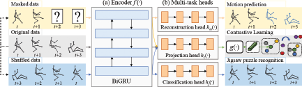
The composition of our pipeline. (a) Encoder. (b) Multi-task heads. Yellow, blue, and green arrows are employed to indicate the pipeline for motion prediction, jigsaw puzzle recognition, and contrastive learning, respectively. In motion prediction, we input masked data and apply the network to reconstruct the original data. In the jigsaw puzzle, we input shuffled data to predict the correct arrangement order. In contrastive learning, we utilize masked and shuffled data as positive samples of the original data to increase feature similarity between positive instances while reducing feature similarity between negative samples.
The composition of our pipeline. (a) Encoder. (b) Multi-task heads. Yellow, blue, and green arrows are employed to indicate the pipeline for motion prediction, jigsaw puzzle recognition, and contrastive learning, respectively. In motion prediction, we input masked data and apply the network to reconstruct the original data. In the jigsaw puzzle, we input shuffled data to predict the correct arrangement order. In contrastive learning, we utilize masked and shuffled data as positive samples of the original data to increase feature similarity between positive instances while reducing feature similarity between negative samples.
3.3 Task-Specific Self-Supervised Learning
Here we introduce two task-specific self-supervised learning methods. With the two methods of motion prediction and jigsaw puzzle, we can learn about the temporal representations of the data. By reconstructing specific joints, motion prediction extracts low-level features, whereas a jigsaw puzzle reconstructs the correct arrangement to extract high-level temporal information.
3.3.1 Motion Prediction
Motion prediction involves predicting a person’s future poses by modeling skeleton dynamics in the context of the past motion sequence. A recurrent encoder-decoder based on Seq2Seq [38] is applied to achieve the desired result. The encoder f (·) reads in sequences and extract representations. In Figure 1, the decoder hm(·) employs the learned representations to reconstruct the whole input sequences by generating sequences.
The input sequences are strengthened by adding random noise during the transformation process. The noise is generated using a Gaussian distribution. This method allows the network to learn more effectively.
For the formulation of motion prediction, assume that the input skeleton sequence is , and we mask from , to for T′ < T to obtain the masked sequence . Then, random noise is input into the sequence to obtain a noisy sequence . We predict the complete and clean skeleton sequence by , where , the mean square error (MSE) is employed to calculate the network’s parameters as follows:
where N means the batch size.
By applying reconstruction, motion prediction enables the network to determine the exact location of each joint by analyzing the motions of the joints, and the relationship between past and future motions helps the network to capture the characteristics in the temporal domain. Furthermore, denoising is aimed at improving the robustness of the input and reducing the overfitting of the network by increasing the randomness of the input.
3.3.2 Jigsaw Puzzle
The goal of solving the jigsaw puzzle problem is to anticipate the proper permutation from shuffled sequences. For the network to learn temporal patterns and sequential orders, we utilize a jigsaw puzzle for skeleton sequences in the temporal domain. From the skeleton sequences, puzzles are generated by dividing P segments into equal parts, with a total of frames in each segment. The segments are shuffled randomly. In addition, we randomly reverse the video to increase the diversity of the temporal transformation as shown in Figure 2(b). By using the network to predict the correct sequence of the disrupted sequence, we train the network to obtain a temporal sequence modeling. Figure 2 shows an example.
After extracting the features through the shared encoder f (·), the classification header hj(·) is applied to obtain the classification results, and then predict the way of being shuffled. MLP is employed as the classification head. The cross entropy loss ℒj constrains the learning process of the network, as follows:
where represents the shuffled data of the original sequence Xi, and yi is the label of the shuffle method.
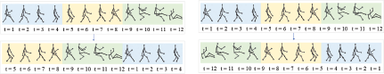
Our design of skeleton jigsaw puzzle. Different segments are represented by different colors, and these segments are randomly shuffled to create various permutations. The goal of solving the jigsaw puzzle problem is to anticipate the proper permutation from shuffled sequences. Using this sequential information, the network can model the characteristics of the temporal domain. (a) Shuffling transformation. We cut the skeleton data into segments and shuffle these segments randomly to create various permutations. (b) Reversing transformation. we randomly reverse the video in temporal dimension.
Our design of skeleton jigsaw puzzle. Different segments are represented by different colors, and these segments are randomly shuffled to create various permutations. The goal of solving the jigsaw puzzle problem is to anticipate the proper permutation from shuffled sequences. Using this sequential information, the network can model the characteristics of the temporal domain. (a) Shuffling transformation. We cut the skeleton data into segments and shuffle these segments randomly to create various permutations. (b) Reversing transformation. we randomly reverse the video in temporal dimension.
Meanwhile, since jigsaw puzzle and action recognition are both high-level tasks, the use of puzzle tasks reduces the task gap between proxy and downstream tasks, making the extracted features more suitable for action recognition.
3.4 Task-Agnostic Self-Supervised Learning
Then, we use contrastive learning to maximize compactness and separability by constrained features. At the same time, contrastive learning is employed to fuse the features obtained from the other two self-supervised tasks, ensuring better performance on downstream tasks.
3.4.1 Contrastive Learning
Our method learns by extracting the same representation from the transformed data and the original data and regulates the feature space by increasing the invariance of the transformation between representations.
With cosine similarity is used to compare the similarity between features, the network learns representations based on SimCLR [1]. Each original sample is subjected to multiple transformations. Our method consists of selecting N randomly selected samples, and applying M different kinds of transformation operators to obtain NM transformed samples. We can then construct pairwise positive and negative pairs for each original sample by transforming its samples.
To map the encoded sequences into the representation manifold, a projection head hc (·) is designed. The features z1, z2, …, zN are extracted from the output of the encoder f (·) and the projection head hc(·) of original data, and be the features of the data transformed from the original data with t from 1 to M. An attention mechanism is applied to dynamically integrate the transformed features.
Attention Mechanism In the feature space built by contrastive learning, we employ a self-attention mechanism to aggregate the features. The previous work [21] employs mean features to aggregate different transformed features. However, some transformations inject too much noise to the original sequences or make the data losing information that is necessary for the downstream tasks. Those transformed features may harm the performance of downstream tasks because of losing information. Therefore, we apply the attention mechanism to assign different weights to different features to be more flexible. This can reduce the influence of noise features and make the training process more robust and stable.
We apply a multilayer perceptron g(·) to assign weights to generated samples. The weight is calculated as follows:
With the weights computed by g(·), we can aggregate the features of generated samples to the attention feature as follows:
After the positive and negative samples are obtained, we use contrastive learning to train the network with InfoNCE loss, which will be described in detail as follows:
InfoNCE Loss We use sim(u, v) = uTv/||u||2||v||2 to determine the cosine similarity between u and v following recent works [1]. The InfoNCE loss function ℒc is defined as follows:
This loss function can increase the feature similarity between positive samples and reduce the similarity between negative samples. Moreover, it has a negative correlation with mutual information. Therefore, optimizing the loss function can extract the mutual information between the original and transformed data. By increasing the mutual information between pairs of positive samples, different information between them can be discarded and consistent representations can be obtained. This consistency can improve the robustness of the network. This information bottleneck mechanism discards a large amount of redundant information while maintaining meaningful information.
As shown in Figure 3, a feature space constraint can be gained with our approach that adapts to any number of transformation operators. We employ two transformation operators that are the same as the motion prediction and puzzle tasks to achieve contrastive learning, i.e., temporal masking, and shuffling.
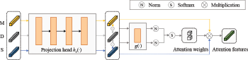
Our method of self-attention contrastive learning. We use yellow, grey, blue, and green to indicate the pipeline for masked data (M), original data (D), shuffled data (S), and attention features, respectively.
Our method of self-attention contrastive learning. We use yellow, grey, blue, and green to indicate the pipeline for masked data (M), original data (D), shuffled data (S), and attention features, respectively.
3.5 Training for Action Recognition
As shown in Figure 4, we add an action classifier C(·) to the encoder f (·) to perform action recognition. Action recognition applies cross entropy loss as follows:
ℒself = ℒm + ℒj + ℒc represents the sum of the three self-supervised learning losses. Three self-supervised tasks are jointly optimized to enable the network to extract diverse features.
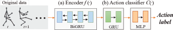
Our method for action recognition. With the features extracted by encoder f (·), we apply an action classifier C(·) for the downstream task.
Our method for action recognition. With the features extracted by encoder f (·), we apply an action classifier C(·) for the downstream task.
As part of the evaluation process, various training methods, such as unsupervised, semi-supervised, and supervised methods, have been experimented with. To use linear evaluation for unsupervised experiments, the encoder only uses the previously introduced self-supervised task as a training task and then trains the action classifier when the encoder is fixed. In a semi-supervised setting, the encoder and classifier are trained together. We train the encoder and fine-tune the network using self-supervised tasks in a fully supervised setting. In addition, we evaluate the performance of transfer learning in the linear evaluation setting and the fine-tuning setting.
Here are detailed introductions of different training strategies.
3.5.1 Linear Evaluation
Through self-supervised learning, we optimize the model without any category labels. We exploit downstream tasks to evaluate the quality of the extracted features. Following SimCLR [1], we attach the linear classifier on top of the frozen encoder to prevent the label information from influencing the encoder for linear evaluation.
3.5.2 Fine-tuning Procedure
For the finetuning process, the weights of the pretrained network are used to initialize, and then the network is finetuned. We exploit the self-supervised learning tasks for the pretraining procedure and employ the labeled data for supervised fine-tuning.
3.5.3 Jointly Training
The jointly training method needs to optimize both the encoder and the classifier. This requires the network to apply both self-supervised tasks and downstream tasks for learning. The loss objective is explained as follows:
where ω is a non-negative constant employed to adjust the ratio of the two-loss functions.
4 Experiment Results
Three datasets: the North-Western UCLA dataset [43], the NTU RGB+D dataset [31], and the PKUMMD dataset [22] are applied for evaluation. With the introduced self-supervised learning tasks, we aim to examine if the feature encoder f (·) can generate suitable feature representations for downstream tasks. Therefore, action classification models are trained in a variety of conditions (i.e., unsupervised, self-supervised, fully supervised, and transfer learning). Besides, We apply our method in different network architectures to show the versatility, i.e., GRU and GCN. Finally, a wealth of experimental analysis allows us to have a deeper understanding of our self-supervised learning tasks and explore the influence of the parameter selection of different self-supervised tasks.
4.1 Dataset and Settings
4.1.1 North-Western UCLA (NW-UCLA) [43]
The dataset includes 1494 videos of 10 individuals performing actions in 10 categories. Body joints have 20 joints, and there are three views of the action data. The first two views are employed for training and the third view is utilized for testing. The videos consist of 1,018 training data and 462 testing data.
4.1.2 NTU RGB+D Dataset (NTU) [31]
There are 56,578 videos in this dataset, with 60 annotations and 25 joints in each frame, performed by 40 subjects. This dataset includes interactions with individual actions as well as pairs. Testing for our methodology is the cross-subject protocol where training is performed on one subject and testing on another. This yields 40,091 training videos and 16,487 testing videos.
4.1.3 PKU Multi-Modality Dataset (PKUMMD) [22]
PKUMMD covers a range of detailed information about human activities and a multi-modality multi-modality 3D understanding of human actions. The actions are organized into 52 action categories and include almost 20,000 instances. There are 25 joints in each sample. The PKUMMD is divided into two versions, part I and part II. In part II, action recognition is more difficult, while in part II, the large view variation causes more skeleton noise. Experiments are conducted according to a cross-subject protocol and on the two subsets.
All sequences of skeletons are downsampled to 60 frames to train the network. Our motion prediction uses the former 70% of frames, which we add random noise to, and mask the latter 30% of frames. When we shuffle the sub-sequences for the skeleton jigsaw, we can select up to 12 ways, including reversing the sequence.
To evaluate different encoder architectures, we used GRU and GCN. Specifically, GRU encoders f (·) are 2-layer bidirectional GRUs with 300 units in each layer and GCN encoders f (·) are 3-layer GCNs with 600 units in each layer. For motion prediction, the reconstruction head hm(·) utilizes two layers of unidirectional GRUs with 600 units and one FC layer. One FC layer is included in the classification head hj(·) for jigsaw puzzles. For contrastive learning, MLPs are used as the projection head hc(·). An FC layer is used for recognition in the classifier C(·). The initial distribution of all networks is random.
The learning rate decreases 0.1 every 100 iterations with the decay rate decreasing from 0.001 with Adam optimizer [25].
4.2 Evaluation and Comparison
By exploring whether the features extracted by our self-supervised enhanced multi-task model (EMS2L) are helpful for action recognition in this section, we raise questions about their relevance. As a result of our varying experimental settings, including unsupervised, semi-supervised, and supervised learning methods, we can evaluate our approach both comprehensively and comprehensively. Comparing the results of our method with state-of-the-art approaches is also included.
4.2.1 Unsupervised Approaches
The unsupervised setting utilizes self-supervised tasks to train the encoder f (·) and then evaluates the feature representation by a linear evaluation mechanism. The linear evaluation mechanism applies a linear classifier to the encoder f (·) with fixed weights to classify the features extracted from it to evaluate the feature representation and utilizes the action recognition accuracy as a measure of the quality of the representation. Note that this encoder f (·) is only optimized with self-supervised tasks and will not be fine-tuned in the linear evaluation protocol. The test configuration includes:
Rand-Unsupervised (Rand-U): Only linear classifiers are trained. This encoder f (·) is randomly initialized, and its weight is fixed throughout training. This is the configuration that we utilize as a baseline.
LongT GAN [52]: This research develops an unsupervised training technique for action recognition that employs skeleton reconstruction for self-supervised learning by using adversarial generative training strategy. It recovers the original data by combining features derived from the original data and randomly covered skeleton data. Following that, in the recognition task, the weights of the encoder are applied. Based on the paper, we build a network.
MS2L [21]: The encoder is trained by a self-supervised task MSS2L, which contains multiple self-supervised tasks.
EMS2L: The encoder is trained first by EMS2L, then the linear classifier is learned while the encoder remains frozen.
Besides, we also perform experiments with recent self-supervised learning methods, i.e., SimCLR [1], MoCo υ2 [13], BYOL [12], and SimSiam [3]. However, those methods are designed for image classification. Thus, the original transformations and structures are more suitable for the characteristics of the picture. Here, to compare with our method, we apply the same architecture and same data transformations for training, i.e., temporal masking, and temporal jigsaw. More detailed information is as followed:
SimCLR [1]:SimCLR applies InfoNCE loss (Equation 5) for contrastive learning and regards data in a batch as negative samples. And the transformed data are positive samples.
MoCo v2 [13]:MoCo υ2 utilizes a queue to store negative features to avoid big batch size in training.
BYOL [12]:BYOL only applies cosine similarity loss between outputs of two neural networks, which one is updated with a slow-moving average of the other network.
SimSiam [3]:SimSiam uses cosine similarity for training and employ stop-gradient operation for preventing collapsing.
In Table 1, the results of the self-supervised learning methods, the baseline (Rand-U), LongT GAN, MS2L, and the proposed EMS2L, are shown in different architectures, different datasets. Our approach outperforms random baselines, LongT GAN, and MS2L in most settings. Comparing with the self-supervised learning tasks shown in Table 1, our method also gets better results in most settings. Our method was successful because it forced the network to extract more useful information. This allows our method to obtain more separable features, which have better compactness and separability. Therefore, we have achieved better results than previous methods. However, our method does not achieve better results in PKUMMD part II dataset. We explain this as the data in the PKUMMD part II dataset contains more noise. And we apply a reconstruction task in self-supervised learning. The reconstruction task utilizes the MSE loss to compute the joint-wise difference. This joint-wise difference is affected by noise. Reconstructing the noisy data may harm the ability of the network. Meanwhile, we notice that GCN with random initialization can achieve higher accuracy than that with GRU. This shows that the randomly initialized GCN also has feature extraction capabilities. On both network architectures, our method can improve its ability to extract features.
Comparison of action recognition results with unsupervised learning approaches.
| Models | Architecture | NW-UCLA | PKUMMD part I | PKUMMD part II | NTU NTU |
|---|---|---|---|---|---|
| SimCLR [1] | GRU | 39.1 | 63.5 | 30.1 | 54.9 |
| MoCo v2 [13] | 49.7 | 62.6 | 27.6 | 47.8 | |
| BYOL [12] | 9.9 | 18.6 | 8.7 | 34.2 | |
| SimSiam [3] | 9.7 | 5.4 | 9.0 | 55.0 | |
| Rand-U | GRU | 52.0 | 51.6 | 28.4 | 40.2 |
| LongT GAN [52] | 74.3 | 67.7 | 25.9 | 52.1 | |
| MS2L [21] | 76.8 | 64.8 | 27.6 | 52.5 | |
| EMS2L | 77.9 | 68.5 | 29.9 | 57.9 | |
| SimCLR [1] | GCN | 70.7 | 73.2 | 34.6 | 54.9 |
| MoCo v2 [13] | 72.2 | 75.9 | 33.9 | 56.0 | |
| BYOL [12] | 49.5 | 43.3 | 15.4 | 36.1 | |
| SimSiam [3] | 73.3 | 72.4 | 33.5 | 55.9 | |
| Rand-U | GCN | 76.1 | 77.2 | 31.8 | 60.3 |
| EMS2L | 78.1 | 77.6 | 29.3 | 61.2 |
In Table 1, we can obverse that if we transfer the image-based self-supervised learning methods into skeleton data directly, the performance is degraded due to the domain gap. SimCLR and MoCo υ2 achieve better action results because these methods apply the same contrastive learning loss as ours. However, BYOL and SimSiam meet serious feature collapsing, which is caused by the gap between skeleton and image data. Skeleton data contains less information than images. Thus, it makes the model more easily collapse to the same outputs.
4.2.2 Semi-Supervised Approaches
With both labeled and unlabeled data, semi-supervised learning can use the structure of unlabeled data to obtain better generalization performance. We utilize unlabeled data to train the encoder f (·), and then apply labeled data to jointly train the classifier C(·).
Rand-Semi Supervised (Rand-SS): Weights are initialized with randomness in the encoder f (·). With the labeled data, all the network weights are then fine-tuned.
LongT GAN [52]: We train the GAN weights with unlabeled sequences and then fine-tune the network using labeled sequences.
S4L [48]: A incorporation of self-supervised and semi-supervised methods is used to train S4L. As an auxiliary task of self-supervised learning, skeleton inpainting is used for 3D action recognition.
ASSL [34]:ASSL combines self-supervised learning and semi-supervised scheme by training the networks via adversarial learning and neighbor feature fusion.
MS2L [21]: With both labeled and unlabeled data, our encoder f (·) is trained together using a jointly training strategy, which means that it is trained with supervised and self-supervised tasks simultaneously.
EMS2L: With selected ω in Equation 7, during training supervised and unsupervised tasks are simultaneously applied to the model.
From Tables 2 and 3, our method consistently improves the baseline, even when we only used small subsets of the datasets.
The model we developed outperforms LongT GAN. LongT GAN reconstructs an entire skeleton with the help of a generative adversarial training strategy. Therefore, the details of skeleton joints are given more attention. Nevertheless, these details might not contribute significantly to action recognition. ASSL exploits label information in neighborhood consistency, we think this method only reduces the distance of the distribution of labeled data and unlabeled data, and for unlabeled data, this method only utilizes the neighborhood consistency for constraint. Our method adopts different self-supervised learning tasks to obtain more meaningful representations. Moreover, joint training provides stronger constraints and avoids overfitting to the labeled data, as well as take advantage of unlabeled data.
Comparison of action recognition results on NW-UCLA dataset with semi-supervised learning approaches.
| Proportion | Models | Architecture | NW-UCLA |
|---|---|---|---|
| 1% | Rand-SS | GRU | 29.4 |
| MS2L [21] | 21.3 | ||
| EMS2L | 37.2 | ||
| Rand-SS | GCN | 28.6 | |
| EMS2L | 33.0 | ||
| 5% | Rand-SS | GRU | 52.5 |
| S4L [48] | 35.3 | ||
| ASSL [34] | 52.6 | ||
| EMS2L | 56.5 | ||
| Rand-SS | GCN | 53.6 | |
| EMS2L | 59.5 | ||
| 10% | Rand-SS | GRU | 57.1 |
| MS2L [21] | 60.5 | ||
| EMS2L | 66.3 | ||
| Rand-SS | GCN | 54.5 | |
| EMS2L | 60.8 |
Comparison of action recognition results on PKUMMD dataset with semi-supervised learning approaches.
| Proportion | Models | Architecture | Part I | Part II |
|---|---|---|---|---|
| 1% | Rand-SS | GRU | 31.8 | 10.1 |
| LongT GAN [52] | 35.7 | 12.3 | ||
| MS2L [21] | 36.4 | 13.0 | ||
| EMS2L | 43.0 | 12.5 | ||
| Rand-SS | GCN | 36.8 | 9.0 | |
| EMS2L | 47.1 | 10.0 | ||
| 5% | Rand-SS | GRU | 67.7 | 21.0 |
| EMS2L | 68.8 | 21.2 | ||
| Rand-SS | GCN | 60.4 | 18.2 | |
| EMS2L | 70.3 | 20.0 | ||
| 10% | Rand-SS | GRU | 75.4 | 24.3 |
| LongT GAN [52] | 69.5 | 25.7 | ||
| MS2L [21] | 70.3 | 26.1 | ||
| EMS2L | 76.4 | 28.5 | ||
| Rand-SS | GCN | 76.1 | 26.6 | |
| EMS2L | 76.0 | 23.3 |
However, from Table 3, we can notice that with 1% labeled data, the accuracy increases 11.2% from 31.8% to 43.0% with the GRU architecture while the accuracy only increases 1.1% with 5% labeled data and 1.0% with 10% labeled data in PKUMMD part I dataset. Also, the accuracy increases 2. 4% from 10. 1% to 12. 5% with GRU architecture while the accuracy only increases 0.2% with 5% labeled data in PKUMMD part II dataset. These results show that with the increase of label data, the performance improvement obtained by the self-supervised task gradually decreases, especially in large datasets. We conjecture this is because our method is mainly to prevent overfitting. When the dataset increases, the overfitting phenomenon is alleviated, so the improvement is not significant.
4.2.3 Supervised Approaches
We apply the self-supervised task encoder f (·) for pretraining in the supervised learning setting, and after pretraining on the encoder f (·), finetune the entire network. We train the encoder f (·) and classifier C(·) using complete training data. Here are the configurations:
Rand-Supervised (Rand-S): We initialize the encoder f (·) and the classifier C(·) randomly.
MS2L [21]: The weights of the encoder f (·) are trained by MS2L, and then the entire network is trained by the action recognition task.
EMS2L: The encoder f (·) is initialized with the weights obtained by the self-supervised task, and the downstream tasks finetune the parameters of the network for action recognition.
SimCLR [1]:SimCLR employs two different transformations of the same data as positive samples to increase the similarity between positive examples and reduce the similarity between different data.
MoCo v2 [13]:MoCo υ2 utilizes a queue to store the features of negative examples, applies contrastive learning pretraining to obtain the weights, and then employs action recognition to train network parameters.
BYOL [12]:BYOL only applies cosine similarity loss to train the encoder f (·) and then we employ action labels for fine-tuning.
SimSiam [3]:SimSiam is an upgraded version of BYOL. It applied cosine similarity to optimize the network so that the two-stream network extracts the same features from different transformations of the same data.
Tables 4 and 5 display the action recognition accuracy on the NW-UCLA and PKUMMD datasets, respectively. Finetuning the encoder after training improves the accuracy of action recognition compared to training from scratch. This result confirms that our method extracts the information demanded by downstream tasks and can better assist in action recognition. The multi-faceted information extracted by this multi-task self-supervised learning has better generalization performance. In comparison with state-of-the-art supervised learning methods, our model achieves better performance on NW-UCLA and is comparable to previous methods on PKUMMD part I and part II.
4.2.4 Transfer Learning Performance
We study the transfer representation learning of EMS2L to see whether it can acquire knowledge about related tasks.
We apply both linear evaluation and finetuning settings to evaluate the performance of transfer learning.
Comparison of action recognition results on the NW-UCLA dataset with supervised learning approaches.
| Models | Architecture | NW-UCLA |
|---|---|---|
| HBRNN-L [7] | RNN | 78.5 |
| SK-CNN [23] | CNN | 86.1 |
| VA-LSTM [49] | LSTM | 70.7 |
| Denoised-LSTM [4] | 80.3 | |
| SimCLR [1] | GRU | 84.4 |
| MoCo v2 [13] | 78.1 | |
| BYOL [12] | 30.7 | |
| SimSiam [3] | 61.4 | |
| Rand-S | GRU | 83.9 |
| MS2L [21] | 85.2 | |
| EMS2L | 85.8 | |
| SimCLR [1] | GCN | 75.7 |
| MoCo v2 [13] | 76.4 | |
| BYOL [12] | 72.7 | |
| SimSiam [3] | 74.8 | |
| Rand-S | GCN | 84.2 |
| EMS2L | 88.0 |
EMS2L: On the source data set, we apply the self-supervised task to train the encoder f (·), and then we employ linear evaluation and finetuning to train the network on the target data set.
Self-supervised learning can learn the common features in different skeleton data distributions so that the representation has a strong transfer performance. Data of different distributions are mapped to the same feature space to obtain high-level action information so that its expressive ability is also adapted to data outside the distribution. The results in Table 6 demonstrate the advantage of our suggested approach, especially when our method is pretrained with the NTU dataset. That is because NTU is much larger than PKU, and pretraining in large dataset extracts more general feature representations. However, when we transfer from NTU dataset to PKUMMD part I dataset, the accuracy drops 5%, though this result is still competitive to previous methods. We conjecture this is because we perform a down-sample transformation in the NTU dataset. This transformation makes a domain gap between PKUMMD part I dataset with NTU dataset in the temporal dimension, which may influence the performance of GRU.
Comparison of action recognition results on the PKUMMD dataset with supervised learning approaches.
| Models | Architecture | Part I | Part II |
|---|---|---|---|
| ST-GCN [47] | GCN | 84.0 | 48.2 |
| VA-LSTM [49] | LSTM | 84.1 | 50.0 |
| SimCLR [1] | GRU | 87.0 | 44.8 |
| MoCo v2 [13] | 86.6 | 43.7 | |
| BYOL [12] | 68.1 | 38.4 | |
| SimSiam [3] | 85.6 | 44.1 | |
| Rand-S | GRU | 81.5 | 44.1 |
| MS2L [21] | 83.4 | 42.4 | |
| EMS2L | 86.4 | 46.6 | |
| SimCLR [1] | GCN | 85.2 | 38.2 |
| MoCo v2 [13] | 82.3 | 34.9 | |
| BYOL [12] | 76.6 | 38.9 | |
| SimSiam [3] | 86.4 | 41.4 | |
| Rand-S | GCN | 86.8 | 42.4 |
| EMS2L | 86.8 | 45.2 |
Comparison of the transfer learning performance.
| Architecture | Source dataset | Part I | Part II | NTU |
|---|---|---|---|---|
| Linear evaluation | ||||
| part I | 68.5 | 27.9 | 39.4 | |
| GRU | part II | 49.5 | 29.9 | 40.3 |
| NTU | 63.5 | 39.8 | 57.9 | |
| part I | 77.6 | 34.7 | 54.2 | |
| GCN | part II | 68.5 | 29.5 | 49.5 |
| NTU | 78.9 | 33.0 | 61.2 | |
| Fine-tuning | ||||
| part I | 86.4 | 46.4 | 70.7 | |
| GRU | part II | 84.7 | 46.6 | 71.2 |
| NTU | 84.4 | 49.2 | 74.9 | |
| part I | 86.8 | 40.8 | 72.7 | |
| GCN | part II | 86.2 | 45.2 | 70.3 |
| NTU | 86.8 | 45.4 | 73.8 |
4.3 Ablation Study
To analyze our proposed approach further, we conduct ablation experiments. The GRU architecture is used for all ablation studies.
4.3.1 Analysis of Self-Supervised Tasks
Throughout this section, we will discuss the importance of each self-supervised task in the training process.
Motion Prediction We test the accuracy of action recognition under different masking ratios of the input sequences, of which some parts of human key points have been masked and zeroed out. Figure 5 shows the accuracy in different settings. It can be observed that as the masking ratio increases, the accuracy of action recognition increases at first and then decreases. Meanwhile, Figure 5 shows the curve of InfoNCE loss between the original and masked sequences. From this, we can see that as the masking ratio increases, the InfoNCE loss between the unmasked sequence and the transformed sequence increases, which implies the mutual information decreases. This is mainly because when the masking ratio is small, motion prediction enables the network to extract the temporal information of the motion for downstream tasks. However, when too much data is covered, the masked sequences have less mutual information with the skeleton data, and it becomes a challenging task for the network to predict future actions through the remaining fragments. The network, therefore, fails to learn useful information from the task, and it also consumes the ability of the network.
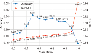
Curves of action recognition accuracy and InfoNCE loss under different masking ratios of the input sequences with 5% of labeled skeleton sequences, respectively (NW-UCLA).
Curves of action recognition accuracy and InfoNCE loss under different masking ratios of the input sequences with 5% of labeled skeleton sequences, respectively (NW-UCLA).
Figure 6 reveals the trend of action recognition precision with the different strength of noise added after 30% frames are masked. It shows a reverse U-shape. We explain it as the light noises injected into the input sequence effectively avoid overfitting for the network, while the large noises would interrupt the learning process.
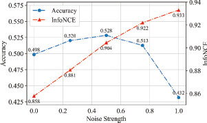
Curves of action recognition accuracy and InfoNCE loss under different noise strength with 5% of labeled skeleton sequences, respectively (NW-UCLA).
Curves of action recognition accuracy and InfoNCE loss under different noise strength with 5% of labeled skeleton sequences, respectively (NW-UCLA).
Jigsaw Puzzles We test the accuracy of action recognition with a different number of segments to shuffle in Table 7. We show the accuracy of action recognition and InfoNCE loss on the NW-UCLA dataset with 5% of labeled skeleton sequences, respectively. Note that with the number of segments increases, the accuracy of action recognition decreases, and the InfoNCE loss between the original and shuffled sequences increases, which means the shuffled sequences lose more mutual information with the original sequences. We conjecture that the larger number of segments results in a more difficult task, which may hinder the performance of action recognition. Besides, small segments lose too much temporal information.
7:
| Transformation | Accuracy | InfoNCE |
|---|---|---|
| 3 Segments | 53.1 | 0.866 |
| 5 Segments | 51.6 | 0.881 |
| 7 Segments | 43.2 | 0.877 |
| 9 Segments | 29.6 | 0.890 |
| 11 Segments | 26.3 | 0.896 |
| w/o Reversing | 53.1 | 0.866 |
| w/ Reversing | 54.5 | 0.883 |
Table 7 shows the impact of whether to perform reversing operation to augment the transformation when the segment number is set to 3. Reversing operation can make the network notice the order of occurrence of action sequences.
Contrastive Learning We study the importance of the attention mechanism for feature fusion. Table 8 shows that attention mechanism can help contrastive learning learn more discriminative representations. We apply the mean feature and attention feature for contrastive learning with unsupervised approaches and supervised learning approaches, respectively. From Table 8, we notice that with the attention mechanism, the performance improves in those settings. However, we notice that in small datasets like NW-UCLA, it improves more from 61.5% to 65.8% with linear evaluation and from 81.4% to 83.3% with fine-tuning. On large datasets, it improves marginally because the noisy features influence more in small datasets and take up a smaller proportion in large datasets. We argue that the attention mechanism provides a more flexible mechanism for feature fusion. In the data transformation, the data may lose a lot of information, which makes the transformed data and the original data quite different. At this time, a large amount of information will be lost if the representations that are required to be consistent between the transformed data and the original data are extracted. The introduction of an attention mechanism can alleviate this effect.
Analysis of contrastive learning with unsupervised and supervised learning approaches.
| Models | NW-UCLA | Part I | Part II | NTU |
|---|---|---|---|---|
| Linear evaluation | ||||
| Mean feature | 61.5 | 68.3 | 26.5 | 39.6 |
| Attention feature | 65.8 | 68.5 | 26.7 | 40.4 |
| Fine-tuning | ||||
| Mean feature | 81.4 | 86.3 | 45.5 | 73.6 |
| Attention feature | 83.3 | 86.3 | 46.6 | 74.0 |
Single self-supervised task and its combinations are displayed in Table 9 for each text. Motion prediction and puzzle tasks are task-specific self-supervised tasks, which extract semantic information from the skeleton data. Among them, motion prediction extracts more low-level joint information, and the puzzle task focuses on global temporal information. As a task-agnostic proxy, contrastive learning intends to find a common manifold between the transformed and original sequences. Through this, the network is trained to acquire deeper representations of inherent features. The best results are achieved when all three tasks are used. The reason is that the features of the extracted tasks maintain more perspectives of the original data statistically.
4.3.2 Training Strategy
We compare the fine-tuning procedure and jointly training strategy in semi-supervised learning. Table 10 shows that for semi-supervised learning, a jointly training strategy achieves better performance than the fine-tuning procedure in the NW-UCLA dataset, PKUMMD part I dataset, and PKUMMD part II dataset. In the NTU dataset, fine-tuning strategy achieves 50.6% with 5% labeled data, while jointly training strategy gets 48.1%. We explain it as jointly training provides stronger constraints and prevents overfitting the small labeled datasets. However, with more data, the over-fitting phenomenon is alleviated.
5 Conclusion
To better apply to the construction of smart infrastructure and analyze from a large amount of unlabeled data collected by sensors, our work proposes a self-supervised learning approach to recognize actions in skeletons. Overfitting can be avoided by integrating multiple tasks to learn more general features and enhancing the tasks with dedicated data transformations. The skeleton dynamics are modeled by motion prediction, whereas temporal patterns are modeled by jigsaw puzzle recognition. Additionally, contrastive learning helps in regularizing the representation space and aids in the acquisition of intrinsic features. Specifically, motion prediction and jigsaw puzzle tasks are used as task-specific proxy tasks to extract semantic-related information. Contrastive learning, as a task-agnostic task, increases the compactness within the class and the separability between classes. We demonstrate that our feature extractor model is a powerful one that outperforms the baseline in a comprehensive analysis of three datasets.
