


The Moving Picture Experts Group (MPEG) has published the geometry-based point cloud compression (G-PCC) standard. It converts the compression of irregular point coordinates to the coding of structured binary octree node occupancy, where the Context-based Adaptive Binary Arithmetic Coding (CABAC) can be applied. The context model, constructed by intra and inter-octree layer information, drives the probability update of the arithmetic coder with a so-called Optimal Binarization with Update On-the-Fly (OBUF) scheme. The original OBUF design, while effective, lacks a probability range limitation for each binary coder, leading to issues in probability estimation accuracy and convergence speed. Moreover, when coding dynamic point clouds, the inter-frame information is not efficiently considered in OBUF, leading to excessive memory consumption for storing and tracking context states. To address these challenges, we propose an initialization strategy for both fine-grained context states (Fine-CtxS) and coarse-grained context states (Coarse-CtxS) in OBUF, alongside an adaptive probability bound determination method for each Coarse-CtxS to confine probability estimation. Furthermore, the paper delves into improvements for inter-frame geometry coding, including the construction of Fine-CtxS, and reducing memory consumption of Fine-CtxS in OBUF. The proposed methods have been adopted in recent G-PCC Edition 2 standardization activities, demonstrating enhanced performance.
1 Introduction
Point clouds have emerged as a pivotal data format for the transmission and storage of immersive visual content and three-dimensional (3D) visual data, as highlighted in the literature [26, 23, 20, 22]. Typically, point clouds encapsulate 3D data in the form of a collection of points, each characterized by its (x, y, z) coordinates, which constitute the point cloud’s geometry. These points are often accompanied by attributes such as color, normal vectors, and reflectance information.
In response to the substantial transmission bandwidth and storage space demands imposed by point clouds, extensive research has been dedicated to the development of efficient Point Cloud Compression (PCC) techniques. Notably, the Moving Picture Experts Group (MPEG) has formalized two PCC standards: the video-based PCC (V-PCC), which leverages 3D to 2D projections, and the geometry-based PCC (G-PCC) [7, 27, 9, 21, 3], which operates directly within the 3D domain.
The G-PCC standard converts the geometry coding of irregular point clouds into binary occupancy signals through octree construction. This conversion facilitates the use of Context-based Adaptive Binary Arithmetic Coding (CABAC) [31], an entropy coding technique that adaptively constructs the context model based on prior encoded symbols. The original formulation of CABAC can entail an exceedingly large number of context states, necessitating a reduction in computational complexity. To this end, G-PCC implements the Optimal Binarization with Update On-the-Fly scheme [8, 18, 12, 17, 11, 13], which efficiently maps numerous fine-grained context states (Fine-CtxS) to a smaller set of coarse-grained context states (Coarse-CtxS) for CABAC. The precision of this probability estimation is pivotal to the coding efficiency.
However, the original OBUF design, while maintaining the probability of each Coarse-CtxS, lacks a defined probability range for each. This oversight results in dramatic probability updates for the Coarse-CtxS, which in turn impacts the accuracy of the probability estimation for each Fine-CtxS. Moreover, the initialization of both Fine-CtxS and Coarse-CtxS commences with a default probability of p0 = 0.5, a practice that may impede the rate of probability convergence, particularly in scenarios involving intra-frame or inter-frame coding.
For the inter-frame dynamic point cloud compression, the OBUF technology adopted in the current G-PCC encompasses both octree-based and trisoup-based coding. Inter-frame coding is achieved by leveraging information from the reference frame to construct the context model. The inter and intraframe information collectively form the Fine-CtxS. However, in the existing octree-based inter-frame geometry coding technology, the enabling of interframe coding and the construction of the Fine-CtxS do not fully consider the information from the reference frame, thus not achieving optimal performance. As for the trisoup-based inter-frame geometry coding technology, the redundant states in the constructed Fine-CtxS lead to excessive memory consumption.
This paper delves into solutions to the aforementioned issues within the OBUF framework. Initially, we propose adjustments to the initialization of probability models of both Fine-CtxS and Corse-CtxS, leveraging the concept of entropy continuation. Subsequently, we introduce adaptively adjusted upper/lower probability bounds as a constraint for each Coarse-CtxS, thereby circumscribing its probability within a specific range. For octree-based interframe geometry coding, we propose an enhancement to the inter-frame enabling determination and the construction of the Fine-CtxS by utilizing uncompen-sated reference frame node information. In the case of trisoup inter-frame geometry coding, we reduce the redundancy of the constructed Fine-CtxS, leverage the redundant information for the classification of the Fine-CtxS and map them to different encoder groups. This approach yields performance gains while significantly reducing memory footprint. These proposed methods have been adopted in recent G-PCC standardization activities [29, 28, 25, 24].
The subsequent sections of this paper are organized as follows: Section II provides an exposition of OBUF and an analysis of its inherent challenges. Section III elaborates on the proposed methods. The paper concludes with Section IV presenting experimental results and Section V offering concluding remarks, respectively.
2 OBUF in G-PCC
The Optimal Binarization with Update On-the-fly (OBUF) mechanism is comprised of three principal components: fine-grained context states modeling, fine-to-coarse context states mapping, and coarse-grained context-based entropy coding. In addition, we briefly introduce the Dynamic OBUF mainly applied in inter-frame coding. Figure 1 illustrates the framework of OBUF. Dashed lines indicate the flow of control or data that is conditional, such as decisions based on the outcome of a previous step (e.g., the selection of Ctxi is based on “Fine-to-Coarse Context Mapping”). Solid lines show the direct progression from one stage to the next without any conditions (e.g., the flow from “Fine-grained context modelling” to “Fine-to-Coarse Context Mapping”). Dashed borders enclose optional or alternative steps that may not be part of the main workflow but are still important for certain scenarios (e.g., “dynamic reduction” might be an optional step depending on the data). Solid borders denote the core stages of the framework where the primary encoding and context mapping take place (e.g., the stages of “Fine-grained context modelling”, “Fine-to-Coarse Context Mapping”, and “Coarse-grained context based entropy coding”).
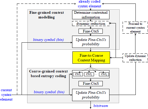
Framework of OBUF. This framework consists of three stages: Fine-grained context modelling, Fine-to-Coarse Context Mapping and Coarse-grained context based entropy coding.
Framework of OBUF. This framework consists of three stages: Fine-grained context modelling, Fine-to-Coarse Context Mapping and Coarse-grained context based entropy coding.
2.1 Fine-grained Context Modeling
In the octree occupancy coding with OBUF, the context information is derived from the occupancy states of 19 already-coded neighbours, which are selected based on their spatial proximity to the current node being encoded. Priority is given to neighbors that shares the face, edge, and vertex in space. Subsequently, considering the requirements for encoding efficiency and memory constraints, G-PCC selects 19 encoded neighbors for further processing. For example, for node bP0, 10 neighbors sharing face, 8 neighbors sharing edge and 1 neighbor sharing vertex are selected. Typically, the number of occupancy states for each node, which has 8 sub-nodes is 8 × 219. These occupancy states obtained directly from the occupancy of neighboring nodes, are termed fine-grained context states (Fine-CtxS). The resulting set of occupancy states remains extensive.
To estimate the probabilities of these numerous Fine-CtxS, OBUF employs an 8-bit unsigned integer to represent the probability of each Fine-CtxS. Theoretically, the probability is adapted to the binary sources through an analysis of the memory channel, which retains L previously encoded symbols. The probability of symbol s from the binary sources is estimated using the Krichevsky-Trofimov formula, as shown in Equation (1) [10]:
where L is a dynamically adjusted memory channel, defined as L = max(5, 1/p, 1/(1 – p)) and capped at 200 symbols to ensure stability.
Following the encoding or decoding process, the 8-bit probability of each Fine-CtxS is updated to pupdate, which is the value closest to as calculated by Equation (1).
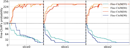
However, the initial probability of each Fine-CtxS is currently set to 127 (corresponding to p = 0.5), which is not conducive to the coding of successive multi-coding units, such as intra-coding of a single frame point cloud or inter-coding of a multi-frame point cloud sequence. As depicted in Figure 2, the Fine-CtxS probability for the “loot” sequence is reset to the default at the beginning of each slice, thereby disrupting the continuity of entropy. Each slice is a specific partition of the point cloud and serves as a fundamental coding unit that is fed into the coder for compression. This practice impedes the rapid convergence of Fine-CtxS’s probability and is not optimal for adapting to diverse binary source distributions.
2.2 Fine-to-coarse Context Mapping
Fine-CtxS’s 8-bit probability divides the probability space into 256 asymmetric ranges. The index of these probability ranges is counted by Idx which is equal to the integer representation of p. The probability quantization technique is employed to condense the probability space into 32 distinct ranges, thereby merging Fine-CtxS instances with closely related probabilities. This consolidation reduces the total number of Fine-CtxS categories without compromising the accuracy of context probability estimation.
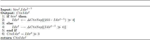
Consequently, thousands of Fine-CtxS are mapped onto a fixed set of N = 32 coarse-grained context states (Coarse-CtxS). The index of each Coarse-CtxS, denoted by CtxIdx, evolves in accordance with the updates to p, as shown in Algorithm 1. The superscript represents the index of symbols to be coded. The probability update mechanism leverages a look-up table, ΔCtxSap, to facilitate this process. From the procedure we can see that when the encoded symbol (i.e., binj) referred by the j-th symbol is 1, the CtxIdx of the adopted Coarse-CtxS increases. Based on the probability updating rule of CABAC, when the previous encoded symbol is 1, the probability of the current symbol to be encoded being 1 will increase. Due to the entropy coding of G-PCC actually uses the probability of 0 to encode the symbol sequence, the probabilities maintained by the Coarse- CtxS decreases monotonically with its index (i.e., CtxIdx).
2.3 Coarse-grained Context-based Entropy Coding
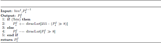
Each Coarse-CtxS possesses an internally maintained probability, denoted by a 16-bit unsigned integer, which is updated in accordance with a probability look-up table: diracLut [1]. This table supplies values for adjusting the probability of zero, contingent upon the first 8 bits of the current value. The process of updating the coder probability is delineated in Algorithm 2, which operates in the inverse updating direction compared to that of Fine-CtxS. We also denote the i-th Coarse-CtxS and its probability as Coarse-CtxS(i) and P (i = 1, 2,32), respectively.
However, when the initial probability is set to 32768 (p = 0.5), Coarse-CtxS encounter a similar issue as Fine-CtxS. In essence, more precise encoding/decoding is imperative to assign distinct initial probabilities to context states, grounded in the principle of entropy continuity.
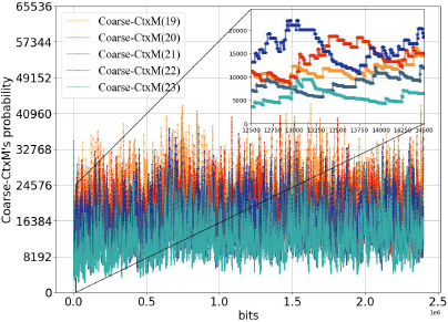
Furthermore, while each Coarse-CtxS encapsulates the low-accuracy probability of a Fine-CtxS, it also possesses its own probability update mechanism. However, these update processes are asynchronous, and there is an absence of a predefined probability range for each Coarse-CtxS. Consequently, the probability of various Coarse-CtxS may fluctuate significantly or update beyond anticipated bounds, as illustrated in Figure 3.
2.4 Dynamic OBUF
Dynamic OBUF is an adaptive mechanism designed to reduce the number of context states dynamically. It leverages the correlation with syntax nodes, classifying the context information derived from previously coded syntax elements into primary and secondary information. The secondary information is then pruned by invoking an update to the dynamic reduction function.
Given that Dynamic OBUF retains the Fine-to-Coarse context mapping procedure and the associated probability updating processes, it is imperative to properly initialize and define the probability range for each context state. This initialization ensures that the mapping and updating operations are conducted within a well-defined probability framework, thus maintaining the integrity and efficiency of the coding scheme.
3 Proposed Method
Building upon the analysis of OBUF, this section introduces a suite of targeted improvements to the existing approach. The challenges identified in Section 2 including the potential discontinuity in entropy due to the reset of probabilities at the beginning of each coding unit, the lack of precision in encoding/decoding that arises from setting initial probabilities to a default value, and the redundant sets in fine-grained context states have directed the development of our method. We address these issues by introducing a statistical-based initialization for independent coding units, establishing upper and lower bounds for Coarse-CtxS probabilities to ensure monotonic decrease, and optimizing the inter-frame context states by considering the occupancy states of both compensated and uncompensated predicted nodes.
3.1 Initialization
For multiple coding, there are two coding units: independent coding units and dependent coding units. Independent coding units do not depend on the entropy state of preceding slices or frames. In contrast, dependent coding units inherit the entropy state from the last update performed in the previous coding unit.
During the initialization phase, the initial probability for a dependent coding unit is ascertained based on the updated probabilities of both Fine-and Coarse-CtxS from the preceding coding unit. In the case of independent coding units, the initialization of their Fine- and Coarse-CtxS’ probabilities is conducted according to the following procedure:
3.1.1 Initialization for Fine-CtxS
We establish a series of statistic-based initial probabilities for the Fine-CtxS of independent coding units. This approach not only underscores the pivotal role of independent coding units in parallel processing but also ensures the rapid convergence of the entropy model’s probability.
3.1.2 Initialization for Coarse-CtxS
For independent coding units, we assign initial probabilities to the 32 Coarse-CtxS individually, derived from theoretical probabilities as illustrated in Equation (2).
where E denotes the entropy error with respect to pi. We consider pi+1 as the smallest probability ensuring this error is confined within ε, calculated using Equation (3).
Commencing with an arbitrarily small p1 and a value of ε = 1.0870 × 10⁻⁴, 256 probabilities spanning the interval [0, 1] are generated through iterative computation using Equation (2). The theoretical probabilities presented in Equation (1) constitute an optimal set of ε-contexts.
Post the mapping process, the optimal initial probability for each Coarse-CtxS is obtained, as shown in Equation (4).
3.2 Upper/Lower Probability Bounds Limitation
A well-initialized probability for each Coarse-CtxS does not inherently guarantee that the probability maintained by Coarse-CtxS(i) decreases monotonically with its index CtxIdx as mentioned in Section 2.2, which can impact the accuracy of Fine-CtxS’s probability estimation.
To address this, we introduce Upper and Lower bounds to constrain the probability of Coarse-CtxS(i). Moreover, the bounds of the probability range for each Coarse-CtxS can be adaptively adjusted, as depicted in Figure 4.
The initial Upper and Lower bounds for each Coarse-CtxS are predicated on the 256 theoretical probabilities pi from OBUF, as defined in Equation (2).
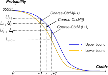
The initial Upper/Lower bounds for Coarse-CtxS(i) are set as follows:
There are three cases for setting the upper/lower bounds of Coarse-CtxS(i)’s probability:
Case1: If the updated probability exceeds the predetermined upper bound of Coarse-CtxS(i), we modify Pi with the upper bound value and adaptively adjust the upper bound .
Case2: If the updated probability falls below the predetermined lower bound of Coarse-CtxS(i), we modify Pi with the lower bound value and adaptively adjust the lower bound .
Case3: If the updated probability lies within the predefined range , no modifications are applied in this iteration.
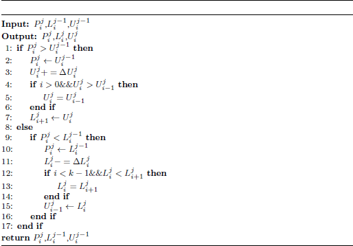
The adjustment of probability boundaries is outlined in Algorithm 3. The adjustments for the Upper/Lower bounds of each Coarse-CtxS during the j-th round are capped at the value of the probability update, i.e., and are less than the updated probability . For implementation simplicity, the adjustments are defined as:
The relationship between probLut and diracLut is given by:
3.3 Dynamic OBUF Context Optimization for Octree Coding
In point cloud geometry inter-frame coding, the octree serves as a crucial coding tool and is an integral part of the coding process based on interframe prediction in current technology. In this section, we first introduce the inter-frame octree geometry coding in G-PCC in Section 3.3.1 and details the proposed improvements in Section 3.3.2, Section 3.3.3 and Section 3.3.4, respectively.
Framework of inter-frame octree geometry coding. It shows how occupancy bo to br are coded and outlines the decision-making of different Fine-CtxS based on the sparsity and the state of inter-frame prediction (i.e., isSparse and isInter2), and the application of corresponding coders with probability updating. Specially, in the proposed improvements, InterNSparse Fine-CtxS and InterSparse Fine-CtxS will be mapped to corresponding Coder based the value of predicted occupancy bPi.
Framework of inter-frame octree geometry coding. It shows how occupancy bo to br are coded and outlines the decision-making of different Fine-CtxS based on the sparsity and the state of inter-frame prediction (i.e., isSparse and isInter2), and the application of corresponding coders with probability updating. Specially, in the proposed improvements, InterNSparse Fine-CtxS and InterSparse Fine-CtxS will be mapped to corresponding Coder based the value of predicted occupancy bPi.
3.3.1 Preliminary: Inter-frame Octree Geometry Coding in G-PCC
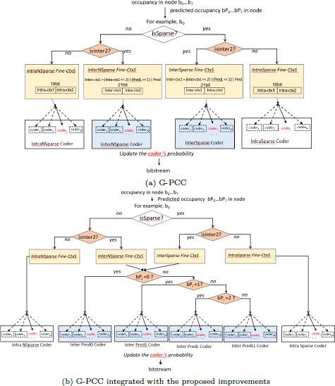
Figure 5a illustrates the existing workflow of octree geometry coding based on inter-frame prediction. The used notations in this section are summarized in Table 1. Here, isSparse refers to the local sparsity of the child nodes to be encoded, determined by the occupancy states of neighboring nodes that have already been encoded. The method for determining the value of isSparse can be referred in [18]. Based on the value of isSparse (0 or 1), two sets of Fine-CtxS are defined: Sparse Fine-CtxS and NSparse Fine-CtxS. Further division is made based on the value of isInter2 (0 or 1), categorizing them into four sets: IntraNSparse Fine-CtxS, InterNSparse Fine-CtxS, IntraSparse Fine-CtxS, and InterSparse Fine-CtxS. isInter2 is calculated as,
Notation of symbols in inter-frame octree geometry coding.
| Notation | Definition |
|---|---|
| isSparse | the local sparsity of the sub-nodes to be encoded |
| isInter | the flag of enabling inter-frame prediction |
| predOcc | the occupancy of predicted nodes in reference frames |
| bi | the occupancy of the sub-node |
| bPi | the occupancy of the sub-node in predicted nodes |
where predOcc indicates whether the predicted node is occupied. The predicted node is the node in the corresponding reference frame that matches the current node. Specifically, if any sub-node bPi of the predicted node is occupied, set predOcc to 1; otherwise, if unoccupied, set predOcc to 0. Furthermore, if inter-frame prediction is enabled, isInter is set to 1; if disabled, isInter is set to 0. Based on the occupancy states of the predicted node, the reference frame octree node occupancy information and the occupied sub-node number information are abstracted into two flags: pred and predL. There are several cases of these flags:
Case1: When the predicted sub-node i is empty (i.e., bPi = 0), we set pred = 0.
Case2: When the predicted sub-node i is non-empty (i.e., bPi = 1), we set pred = 1. In this case, depending on the number of points within the predicted node, two sub-cases are considered:
- (a)
Subcase1: When the number of points exceeds the threshold th, it is strongly occupied and predL = 1.
- (b)
Subcase2: When the number of points does not exceed the threshold th, it is not strongly occupied and predL = 0.
- (a)
The above pred and predL are used as 2-bit inter-frame information, plus 19 bits of intra-frame information, and finally constitute a total of 21 bits of information for the InterNSparse Fine-CtxS and InterSparse Fine-CtxS. The 19 bits of intra-frame information refer to the primary and secondary information mentioned in Section 2.4, denoted as intra-ctxl and intra-ctx2 respectively. When a node utilizes the InterNSparse Fine-CtxS and InterSparse Fine-CtxS, the number of the original occupancy states for each node of 8 sub-nodes is about 8 × 221. For IntraNSparse Fine-CtxS and IntraSparse Fine-CtxS, they consist of only 19 bits of information. The number of the original occupancy states for each node of 8 sub-nodes is about 8 × 219.
In summary, the multi-frame point cloud entropy coding process begins with the evaluation of the isSparse variable, which is based on the sparsity of the sub-nodes within the frame. This is followed by the determination of the isInter’2 variable, which considers the inter-frame enabling flag and the occupancy states of predicted nodes. Depending on the values of isSparse and isInter2, the corresponding Fine-CtxS set is determined, which is then linked to their corresponding group encoders. The group encoders have their respective dynamic OBUF models as described in Section 2.1. Subsequently, The group encoder is mapped to a binary encoder, and the resulting encoder coderi performs entropy coding on the symbols. This streamlined approach ensures an efficient coding process that is sensitive to both intra-frame and inter-frame contexts.
Current octree-based inter-frame coding scheme as described in Section 3.3.1, which multiply the number of inter-frame context states fourfold compared to intra-frame models, leading to excessive storage requirements and hardware strain. Moreover, they neglect the correlation between sparse and non-sparse states across frames, thereby limiting the coding efficiency. To address these issues, we propose three enhancements, including the determination of inter-frame context enabling, improvement of the inter-frame context states based on the occupancy states of predicted of nodes, and mapping of a shared encoder group for sparse and non-sparse inter-frame context states, as depicted in Figure 5b.
3.3.2 Determination of the Inter-Frame Context Enabling
Contextualization significantly influences the probability models employed within CABAC, thereby directly impacting the compression efficiency. Currently, the enabling of the inter-frame context only depends on the compensated reference node information (i.e., predOcc). To consider the inter-frame information more comprehensively, the information of uncompensated reference nodes predOccUnComp is also considered to determine isinter2. predOccUnComp indicates whether the predicted node in the reference frame without motion compensation is occupied. The determination of its value is similar to predOcc. If any sub-node of the predicted node in the reference frame without motion compensation is occupied, set predOccUnComp to 1; otherwise, if unoccupied, set predOccUnComp to 0. As such, isinter2 is calculated as follows:
3.3.3 Improvement of the Inter-frame Context States
The occupancy states of uncompensated predicted nodes, denoted as bPiUn-Comp, is calculated:
where NodePointsUnComp[i] represents the number of points in the uncompensated predicted sub_node[i]. Based on the number of points in uncom-pensated prediction nodes, we propose that the uncompensated inter-frame predicted information is classified into the following two cases:
Case1: Uncompensated sub_node[i] is predicted as unoccupied and bPiUnComp = 0.
Case2: Uncompensated sub_node[i] is predicted as occupied and bPiUn-C omp = 1.
Further, we use the 1-bit information bP iUnComp to replace the 2-bit information of pred and predL in InterSparse Fine-CtxS and InterNSparse Fine-CtxS mentioned in Section 3.3.1. Specifically, we replace
into
This approach improves the inter-frame context state by reducing half of the memory footprint from storing 221 states to 220 states without decreasing the coding efficiency of the system.
3.3.4 Encoder Group Mapping
Based on the number of points in predicted nodes, Lasserre et. al [19] proposes to represent the occupancy states of predicted nodes as,
where NodePoints[i] is the number of points in predicted sub_node[i], and thj denotes the threshold. thj depends on the size of the node. If NodeSize represents the size of the node, then:
Further, the occupancy states of predicted nodes is categorized into the following four cases:
Casel: sub_node[i] is predicted as unoccupied when bPi = 0.
Case2: sub_node[i] is predicted as occupied when bPi = 1.
Case3: sub_node[i] is predicted as strongly occupied when bPi = 2.
Case4: sub_node[i] is predicted as very strongly occupied and bPi = 3.
Based on these cases, we propose to map different inter-frame contexts to different encoder group as shown in Table 2. The encoder groups correspond to their respective dynamic OBUF models. This method utilizes the inter-frame non-motion compensation node information to the greatest extent, thereby further enhancing the geometry coding efficiency of G-PCC.
Mapping of Inter-frame Contexts to Encoder Groups in Inter-frame Octree Coding.
| Context | Encoder Group |
|---|---|
| IntraNSparse Fine-CtxS | IntraNSparse Encoder |
| IntraSparse Fine-CtxS | IntraSparse Encoder |
| InterNSparse Fine-CtxS | bPi= 0: InterPredO Encoder |
| bPi= 1: InterPred1 Encoder | |
| bPi= 2: InterPredL Encoder | |
| bPi= 3: InterPredLL Encoder | |
| InterSparse Fine-CtxS | bPi= 0: InterPredO Encoder |
| bPi= 1: InterPred1 Encoder | |
| bPi= 2: InterPredL Encoder | |
| bPi= 3: InterPredLL Encoder |
3.4 Dynamic OBUF Context Optimization for Trisoup Coding
In point cloud inter-frame geometry coding, trisoup coding, as another important geometry coding tool, has rapidly developed and is widely applied in the current G-PCC standard [15, 14, 16]. In this section, we first introduce the inter-frame trisoup geometry coding in G-PCC in Section 3.4.1 and details the proposed improvements in Section 3.4.2 and Section 3.4.3, respectively.
3.4.1 Preliminary: Inter-frame Trisoup Geometry Coding in G-PCC
Trisoup geometry coding is mainly used to process vertex information, including the existence and the positions of vertices.
Both intra-frame and inter-frame coding use the OBUF technique for entropy coding. Compared to intra-frame coding, the context construction method of inter-frame coding has some particularities. Specifically, the interframe context states take into account the current intra-frame context states of the symbol to be encoded and the current vertex prediction information. The vertex prediction information refers to the vertex information of the reference frame obtained through frame matching.
Figure 6a illustrates the coding process of trisoup vertex existence information. The used notations in this section are summarized in Table 3. The variable islnterGood is an indicator of the quality of inter-frame prediction. When inter-frame prediction is enabled, isInterGood takes a binary value (0 or 1), signifying the prediction of neighboring compensated and uncompensated vertices is well-predicted or poorly predicted. Depending on the value of isInterGood, the contexts are bifurcated into two primary sets: intra-frame Fine-CtxS and inter-frame Fine-CtxS.
Notation of symbols in inter-frame trisoup geometry coding.
| Notation | Definition |
|---|---|
| isInterGood | an indicator of the quality of inter-frame prediction |
| T riSoupV erticesPred | the position information of the compensated vertice |
| nBadPredRef | the count of inaccurately predicted uncompensated vertices among neighboring vertices |
| colocatedV ertex | the uncompensated reference vertex information |
Further subdivision of the inter-frame context is determined by TriSoup-V erticesPred, which denotes the position information of the compensated vertices. This leads to the creation of two subsets within the inter-frame context: Inter context 1 for well-predicted compensated vertices and Inter context 2 for poorly predicted ones.
The categorization of inter-frame prediction information is contingent upon the prediction quality of neighboring uncompensated vertices (i.e., nBadPredRef) and the uncompensated reference vertex information (i.e., colocatedVertex). The classification is as follows:
- NoPred: When the prediction of neighboring uncompensated vertices is poor (i.e., nBadPredRef ≤ 0), the information from the uncompensated reference vertex is not utilized and the vertex to be encoded is not predicted.Figure 6
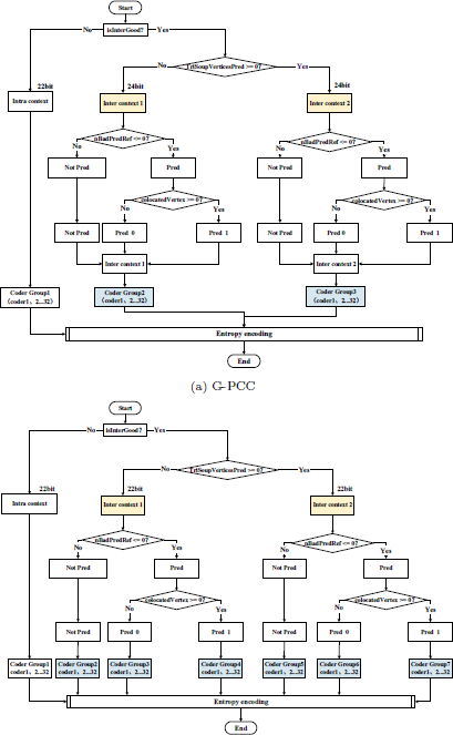
Framework of inter-frame trisoup geometry coding. It goes through a series of conditional branches based on the inter-frame enabling, the position information, the prediction quality of uncompensated vertices and the presence of co-located vertices (i.e., isInterGood, TriSoupVerticesPred, nBadPredRef and colocatedV ertex). Each branch maps different contexts to corresponding coder group for entropy coding. Specially, in the proposed improvements, nBadPredRef and colocatedV ertex are no longer contained in Inter context 1 and Inter context 2, instead of guiding the mapping of contexts to the corresponding Coder Groups.
Figure 6Close modalFramework of inter-frame trisoup geometry coding. It goes through a series of conditional branches based on the inter-frame enabling, the position information, the prediction quality of uncompensated vertices and the presence of co-located vertices (i.e., isInterGood, TriSoupVerticesPred, nBadPredRef and colocatedV ertex). Each branch maps different contexts to corresponding coder group for entropy coding. Specially, in the proposed improvements, nBadPredRef and colocatedV ertex are no longer contained in Inter context 1 and Inter context 2, instead of guiding the mapping of contexts to the corresponding Coder Groups.
PredO: In cases where the prediction of neighboring uncompensated vertices is satisfactory (i.e., nBadPredRef > 0), and the value of the uncompensated reference vertex information is less than zero (i.e., colocatedVertex ≤ 0), the vertex to be encoded is predicted to be zero.
Pred1: Similarly, when the neighboring uncompensated vertex prediction is good (i.e., nBadPredRef > 0), and the value of the uncompensated reference vertex information is zero or greater (i.e., colocatedVertex ≥ 0), the vertex to be encoded is predicted to be one.
Ultimately, both intra-frame and inter-frame information are consolidated into three distinct sets of group encoders, each aligned with their respective dynamic OBUF models. This structured approach ensures an coding process that adapts to the varying degrees of prediction accuracy encountered in multi frames.
Following our enhancements to the context states optimization for octree-based geometry coding, which alleviates the excessive proliferation of context states, we turn our attention to the trisoup-based inter-frame coding. Similar to the octree approach, the current trisoup geometry coding (i.e., Section 3.4.1) faces challenges with an inflated number of inter-frame context states being six times that of intra-frame models, which leads to significant storage demands and potential interference among shared coding resources. To streamline this process, we propose two straight improvements: a reduction in the number of inter-frame context states and a subsequent mapping of encoders as shown in Figure 6b. These improvements, detailed in the following sections, are designed to harmonize with our previous optimizations, thereby creating a unified strategy to enhance the efficiency of geometry coding across both octree and trisoup inter-frame coding.
3.4.2 Reduction of the Number of Inter-frame Context States
Current intra-frame context states use an independent set of models, which can be constructed using existing methods [32, 3O, 6]. For inter-frame context states as described in Section 3.4.1, Inter context 1 and Inter context 2 are distincted by the variable T riSoupVerticesPred. Compared to this scheme, we propose to no longer add 2-bit inter-frame information of nBadPredRef and colocatedVertex to generate new context states. In this time, the interframe contexts are the same as the intra-frame contexts. Therefore, the memory footprint is one-fourth of the original by reducing 224 states to 222 states. The saved 2 bits are used to classify the context states and the subsequent encoder group mapping are described in the next subsection.
3.4.3 Encoder Group Mapping
Intra-frame context states are mapped to Coder 1 and inter-frame context states are mapped to Coder 2 to Coder 7. Detailed mapping are shown in Table 4. Based on the above information, the context states and encoder group are determined. This method properly utilizes the inter-frame nonmotion compensation node information to reduce the redundancy of inter-frame context states, reducing the memory footprint without decreasing the coding efficiency of the system.
4 Experimental Results
The performance of the proposed methods is assessed utilizing the G-PCC reference software TMC13v20, within a simulation environment constructed following the Common Test Conditions (CTC) guidelines [2][4]. The evaluation spanned two compression scenarios: lossless-geometry-lossless-attribute, denoted as CW, and lossy-geometry-lossy-attribute, denoted as C2. The test content for the integration of the refined initialization strategy and the Upper/Lower Probability Bounds Setting includes Static Objects and Scenes with subcategories of Solid, Dense, Sparse, and Scant; and Dynamic Acquisition with subcategories of Am. Frame spinning, Am. Frame non-spinning, and Am. Fused.
For inter-frame coding, the test content includes multi-frame Dynamic Humans [5] classified as categories A (loot, redandblack, soldier and queen), B (longdress), and C (basketball player and dancer player).
The metrics of bits per input point (bpp) and Bjøntegaard delta bit rate (BD-rate) are adopted to assess the efficiency of our compression algorithms. The distortion of the geometry was further evaluated through point-to-point PSNR (D1 PSNR) and point-to-plane PSNR (D2 PSNR) measurements.
As shown in Table 5 and Figure 7, the integration of the refined initialization strategy and the Upper/Lower Probability Bounds Setting has yielded distinct improvements in coding efficiency across different conditions. Specifically, in Figure 7, we show the R-D curves of G-PCC and the proposed mothod of loot. Due to the same PSNR across various bpps, the values of bpps are labeled in the figure. We can see that the bpps of the proposed methods are all lower than those of G-PCC, showing its effectiveness. In Table 5, under the lossless-geometry-lossless-attribute condition, the average bpp has demonstrated a gain of 0.3%. Under the lossy-geometry-lossy-attribute condition, the BD-rate for D1 and D2 has achieved average gains of 1.67% and 1.43% for octree-based geometry coding, respectively. For trisoup-based geometry coding, the BD-rate for D1 and D2 has achieved average gains of 4.08% and 4.06%, respectively. For the integration of the refined initialization strategy and the Upper/Lower Probability Bounds Setting for Fine- and Coarse-Context states, the gains show differences based on the sparsity of point cloud. Generally, under the lossy geometry compression condition, the point cloud will be quantized to some extent before them are fed into the codec, showing more denser distribution compared with lossless geometry compression condition. Therefore, the correlation between nodes is stronger and thus the proposed optimization of nodes’ occupancy-based context modelling shows more gains. Furthermore, for all conditions, the gains of the proposed method also become more evident with denser test point clouds.
Bpp and BD-rate reduction results of the integration of the refined initialization strategy and the Upper/Lower Probability Bounds Setting v.s. existing G-PCC geometry coding.
| Experimental conditions | |||||
|---|---|---|---|---|---|
| category | Octree Geom.CW | Octree Geom.C2 | Trisoup Geom.C2 | ||
| geometry bpip | D1 BD-rate | D2 BD-rate | D1 BD-rate | D2 BD-rate | |
| Solid average | 98.52% | -2.60% | -2.62% | -4.61% | -4.63% |
| Dense average | 99.07% | -2.11% | -2.09% | -4.05% | -4.01% |
| Sparse average | 99.55% | -1.49% | -1.49% | -4.12% | -4.04% |
| Scant average | 99.82% | -0.55% | -0.55% | -3.79% | -3.79% |
| Am-fused average | 99.79% | -0.85% | -0.84% | ||
| Am-frame spinning average | 99.78% | -0.97% | -0.96% | ||
| Am-frame non-spinning average | 99.81% | -6.02% | |||
| Overall average | 99.72% | -1.67% | -1.43% | -4.08% | -4.06% |
| Avg.Enc Time | 100.91% | 101.28% | 100.58% | ||
| Avg.Dec Time | 102.08% | 103.03% | 100.55% | ||
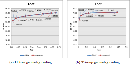
R-D curve comparison of Loot with G-PCC and the proposed improvements of integration of the refined initialization strategy and the Upper/Lower Probability Bounds Setting.
R-D curve comparison of Loot with G-PCC and the proposed improvements of integration of the refined initialization strategy and the Upper/Lower Probability Bounds Setting.
The dynamic OBUF context state optimization, when applied to octree-based geometry coding, has resulted in a BD-rate reduction of 2.41% for D1 and 2.41% for D2 under the C2 condition as shown in Table 6 and Figure 8. For trisoup-based geometry coding, the respective BD-rate improvements stand at 0.14% for D1 and 0.15% for D2 under C2. As the motion amplitude of different test sequences increases, the gains from proposed dynamic OBUF context state optimization become more significant. This is because larger motion amplitudes lead to more inaccurate motion estimation and compensation in G-PCC, thus the proposed dynamic OBUF context using information of uncompensated reference nodes provides more gains. To demonstrate this relationship, we offer the gains of all test sequences in Table 6. Furthermore, we utilized the motion estimation in G-PCC to check motion amplitudes of test point cloud sequences. For the sequences with less significant motion amplitudes (i.e., queen and solider) have less gains compared with other sequences with more significant motion amplitudes. Moreover, the memory footprint for storing the context is reduced to one-fourth of the original consumption as mentioned in Section 3.4.2.
BD-rate reduction results of proposed dynamic OBUF context state optimization v.s. existing G-PCC geometry coding.
| Experimental conditions | ||||
|---|---|---|---|---|
| category | Octree Geom.C2 | Trisoup Geom.C2 | ||
| LU BD-rate | U2 BD-rate | D1 BD-rate | U2 BD-rate | |
| loot | -2.57% | -2.61% | -0.35% | -0.34% |
| redandblack | -2.52% | -2.57% | -0.19% | -0.20% |
| soldier | -2.25% | -2.22% | -0.12% | -0.16% |
| queen | -1.84% | -1.86% | 0.35% | 0.26% |
| A average | -2.30% | -2.27% | -0.08% | -0.11% |
| B (i.e., longdress) average | -2.45% | -2.50% | -0.17% | -0.17% |
| basketball player | -2.69% | -2.72% | -0.30% | -0.29% |
| dancer player | -2.54% | -2.57% | -0.18% | -0.18% |
| C average | -2.62% | -2.65% | -0.24% | -0.23% |
| Overall average | -2.41% | -2.41% | -0.14% | -0.15% |
| Avg.Enc Time | 101.45% | 100.18% | ||
| Avg.Dec Time | 102.33% | 100.65% | ||
4.1 Ablation Study
In this section, We design the ablation study to evaluate the performance of the refined initialization strategy and the Upper/Lower Probability Bounds Setting, respectively. The dynamic OBUF context state optimization is integrated in G-PCC as an intact component, which can not be separated to implement the ablation study. As shown in Table 7, the integration of the refined initialization strategy has yielded improvements in coding efficiency across different conditions. Specifically, under the lossless-geometry-lossless-attribute condition, the average bpp has demonstrated a gain of 0.01%. Under the lossy-geometry-lossy-attribute condition, the BD-rate for D1 and D2 has achieved average gains of 0.37% and 0.18% for octree-based geometry coding, respectively. For trisoup-based geometry coding, the BD-rate for D1 and D2 has achieved average gains of 2.40% and 2.38%, respectively. Table 8 shows the integration of the Upper/Lower Probability Bounds Setting also yielded improvements in coding efficiency across different conditions. Specifically, under the lossless-geometry-lossless-attribute condition, the average bpp has demonstrated a gain of 0.3%. Under the lossy-geometry-lossy-attribute condition, the BD-rate for D1 and D2 has achieved average gains of 1.00% and 1.00% for octree-based geometry coding, respectively. For trisoup-based geometry coding, the BD-rate for D1 and D2 has achieved average gains of 0.58% and 0.59%, respectively.
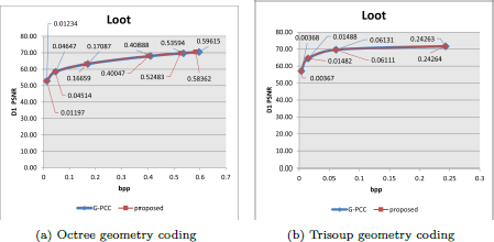
R-D curve comparison of Loot with G-PCC and the proposed improvements of dynamic OBUF context state optimization.
R-D curve comparison of Loot with G-PCC and the proposed improvements of dynamic OBUF context state optimization.
5 Conclusions
This research introduces enhancements to the MPEG G-PCC standard, specifically addressing the limitations of the original OBUF design. The refinements to context state initialization and the introduction of adaptive probability bounds have significantly improved the accuracy and convergence of probability estimations. Additionally, the paper presents innovative approaches to inter-frame geometry coding, optimizing the use of reference frame information and reducing memory footprint. The experimental results validate the performance improvements achieved by integrating these enhancements into the G-PCC standard.
Bpp and BD-rate reduction results of the integration of the refined initialization strategy v.s. existing G-PCC geometry coding.
| Experimental conditions | |||||
|---|---|---|---|---|---|
| category | Octree Geom.CW | Octree Geom.C2 | Trisoup Geom.C2 | ||
| geometry bpip | D1 BD-rate | D2 BD-rate | D1 BD-rate | D2 BD-rate | |
| Solid average | 99.95% | -0.39% | -0.40% | -2.47% | -2.49% |
| Dense average | 99.99% | -0.35% | -0.34% | -2.26% | -2.25% |
| Sparse average | 100.00% | -0.16% | -0.15% | -2.61% | -2.53% |
| Scant average | 100.00% | -0.01% | -0.01% | -2.33% | -2.34% |
| Am-fused average | 100.00% | -0.02% | -0.02% | ||
| Am-frame spinning average | 99.97% | -0.16% | -0.16% | ||
| Am-frame non-spinning average | 99.98% | -3.87% | |||
| Overall average | 99.99% | -0.37% | -0.18% | -2.40% | -2.38% |
| Avg.Enc Time | 99.99% | 100.11% | 100.98% | ||
| Avg.Dec Time | 99.56% | 101.03% | 100.12% | ||
Bpp and BD-rate reduction results of the integration of the Upper/Lower Probability Bounds Setting v.s. existing G-PCC geometry coding.
| Experimental conditions | |||||
|---|---|---|---|---|---|
| category | Octree Geom.CW | Octree Geom.C2 | Trisoup Geom.C2 | ||
| geometry bpip | D1 BD-rate | D2 BD-rate | D1 BD-rate | D2 BD-rate | |
| Solid average | 98.61% | -1.40% | -1.40% | -0.69% | -0.70% |
| Dense average | 99.07% | -1.37% | -1.37% | -0.66% | -0.66% |
| Sparse average | 99.55% | -1.19% | -1.19% | -0.44% | -0.48% |
| Scant average | 99.82% | -0.55% | -0.55% | -0.52% | -0.53% |
| Am-fused average | 99.79% | -0.84% | -0.84% | ||
| Am-frame spinning average | 99.83% | -0.73% | -0.73% | ||
| Am-frame non-spinning average | 99.83% | -0.93% | |||
| Overall average | 99.72% | -1.00% | -1.00% | -0.58% | -0.59% |
| Avg.Enc Time | 101.56% | 101.08% | 98.97% | ||
| Avg.Dec Time | 102.23% | 100.90% | 100.19% | ||
