


Kleibergen and Zhan (2020) propose a new approach to test consumption-based asset pricing models that is robust to the “useless” factor problem, i.e., concluding too often that a factor is priced when the factor is actually uncorrelated with the test assets and is not priced. I show that even when factor correlation is economically large and significant (think of 0.40 and larger), their testing approach lacks power in small samples to detect sufficient factor correlation or to find that a factor is priced. I propose simple remedies that help to achieve robust and powerful asset pricing tests.
Kleibergen and Zhan (2020) worry that recently proposed alternative consumption measures (Jagannathan and Wang, 2007; Kroencke, 2017; Parker and Julliard, 2005; Savov, 2011) are only poorly correlated with stock returns. They claim that the popular textbook methods (Campbell, 2017; Campbell et al., 1997; Cochrane, 2005; Ferson, 2019) cannot be trusted when risk factors are “useless” (i.e., uncorrelated with stock returns) and when the sample size is small (as is often the case in consumption-based pricing). In considering these claims, they propose a new testing methodology that is robust to “useless” factors. They illustrate their method on a short sample of the dataset studied in Kroencke (2017). Using this new methodology, they can neither confirm nor reject the idea that the consumption factor helps explain stock returns (Kleibergen and Zhan, 2020, p. 547).
For the empirical application they consider, I show that their methodology lacks the power to provide inference on the factor correlation, the coefficient of relative risk aversion, or the price of risk. At the same time, traditional inference using GMM-based tests of the non-linear model, or Fama–MacBeth/Shanken t-statistics for the linearized model, perform considerably better than is stated in Kleibergen and Zhan (2020). The textbook methods are often (but not always) trustworthy and are always more powerful in detecting “useful” factors. Furthermore, simple bootstrap confidence intervals are always trustworthy and remain powerful. This paper aims to illustrate the properties of the different methods in empirically relevant cases so that applied researchers can make informed decisions on which method to use in consumption-based asset pricing.
GMM-based tests of the non-linear model:Kleibergen and Zhan (2020) consider GMM-based tests (Hansen, 1982) of the non-linear version of the consumption-based model when the market excess return is the only test asset. If an estimate of the coefficient of relative risk aversion is significantly different from zero, in an economically plausible range, and the pricing error is small, such a finding is interpreted as evidence that the consumption factor helps to explain the equity premium. The core of the problem is that the coefficient of relative risk aversion cannot be identified when the factor is “useless.” Estimates will come with a non-standard distribution, which is also wider than the distribution of a “useful” factor. Because GMM standard errors assume that a factor is “useful,” one might too often conclude that the factor helps to explain the equity premium when the factor is actually “useless.”
Kleibergen and Zhan (2020) claim that the correlation of alternative consumption measures is indeed insufficient to trust GMM standard errors, even though factor correlation is economically and statistically significant for several of the consumption measures considered.1 My paper shows that their test for sufficient factor correlation (called the GMM-rank test) is almost impossible to pass, regardless of whether a factor is “useless” or “useful” and highly correlated with asset returns.
I illustrate the issue in Figure 1, where I report simulation results of the GMM-rank test executed with the same code and the same settings as in Kleibergen and Zhan (2020). The y -axis shows the simulation-based probability to reject the null hypothesis that a factor is “useless.” The x -axis varies the population factor correlation coefficient with the consumption factor from zero (“useless”) up to 1.00 (the “most useful” factor one can hope for).2The flat line shows that the GMM-rank test is unable to detect sufficient factor correlation for any amount of factor correlation, even when factor correlation is perfect.3Insufficient factor correlation cannot bethe problem.
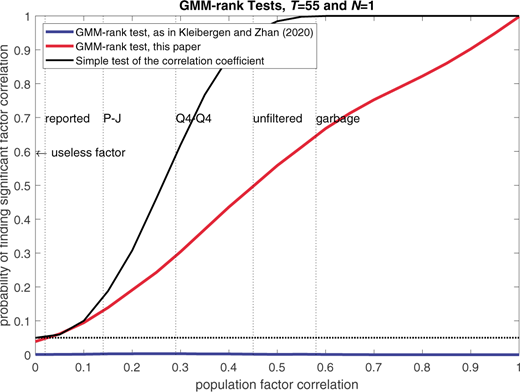
The Power of GMM-Rank Tests.
The Power of GMM-Rank Tests.
Instead, I show that the failure to detect “useful” factors is due to a bad GMM objective function. It has two corner solutions, where the statistical software used reaches the limit of numerical precision and rounds the GMM objective functions arbitrary to zero. Because the test statistic is arbitrary set to zero somewhere, it is impossible to find a test statistic larger than the critical value and reject the hypothesis that there is a lack of factor correlation. The situation is known as the “GMM trap” (see Figure 2 for an illustration with the empirical data).4
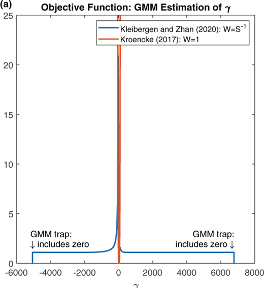
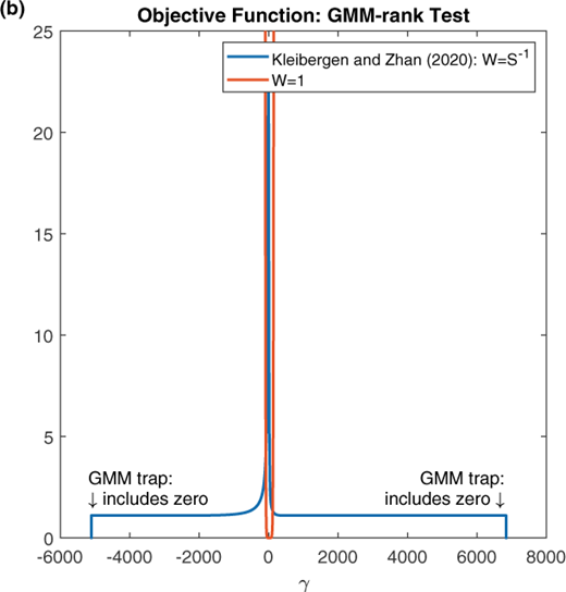
GMM Objective Functions and the GMM Trap.
GMM Objective Functions and the GMM Trap.
The “GMM trap” also plagues the novel method for robust estimation of the coefficient of relative risk aversion in consumption-based asset pricing models. Kleibergen and Zhan (2020) propose replacing standard GMM-based inference with the GMM-Anderson-Rubin (GMM-AR) test to obtain a “useless” factor robust test. The GMM-AR test searches for all possible values of the coefficient of relative risk aversion where a test of a zero moment condition (the “J-test”) cannot be rejected. This region is then used to determine confidence intervals for the coefficient of relative risk aversion.
When the factor is “useful,” and the sample is large enough, there should be a single parameter region where the J-test cannot be rejected, which results in a bounded confidence interval. Unbounded (or disjointed) confidence intervals mean that the J-test cannot be rejected in a single region, which is interpreted as evidence of insufficient factor correlation. Again, because the objective function is arbitrarily set to zero at multiple regions, the GMM-AR confidence intervals are likely to appear unbounded. But these unbounded confidence sets do not necessarily reflect poor factor correlation but rather the ill-conditioned GMM objective function. While the GMM-AR test is robust to the “useless” factor problem, this approach lacks the power to detect “useful” factors in empirical applications Figure 3). This brings me to the main critique of this paper. A “useless” factor robust test procedure is not helpful for applied research if the test does not allow for the detection of a “useful” factor.
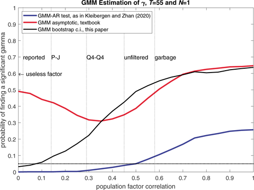
The Power of GMM-Based Inference on the Coefficient of Relative Risk Aversion.
The Power of GMM-Based Inference on the Coefficient of Relative Risk Aversion.
I discuss remedies that allow one to conduct inference that is “useless” factor robust and powerful. (1) I propose to use a modified test for sufficient factor correlation (GMM-rank test). This version does not weight the moment condition(s) and has no corner solutions. A simulation experiment shows that the corrected GMM-rank test is more accurate and can differentiate between “useless” and “useful” factors (see Figure 1). A direct test of the correlation coefficient, similar to the one reported in Savov (2011), is even more powerful in detecting “useful” factors (see Figure 1). (2) I show that applying the GMM-AR test to the linearized version of the consumption-based asset pricing model limits the risk of encountering an ill-conditioned GMM objective function. However, the confidence intervals of the GMM-AR test are large, which indicates a relatively low power of this approach. (3) I point out that there is an easy-to-implement alternative available. Bootstrapped confidence intervals, as implemented in Burnside (2011) for linear models, are robust to the “useless” factor problem and come with more power to detect “useful” factors (Figure 3). If a factor is “useful,” the bootstrapped confidence interval will be comparable to those based on asymptotic inference (if the sample size is large enough). If a factor is “useless,” the bootstrapped estimates will be non-standard distributed but still centered around zero (Figure 4). Confidence intervals based on the bootstrap distribution are large and likely to include the value of zero. Importantly, the bootstrap confidence intervals do not over-reject the coefficient of relative risk aversion being different from zero as one benchmarks the point estimate with the distribution of a “useless” factor and not with that of a “useful” factor (as would be the case when relying on asymptotic standard errors).
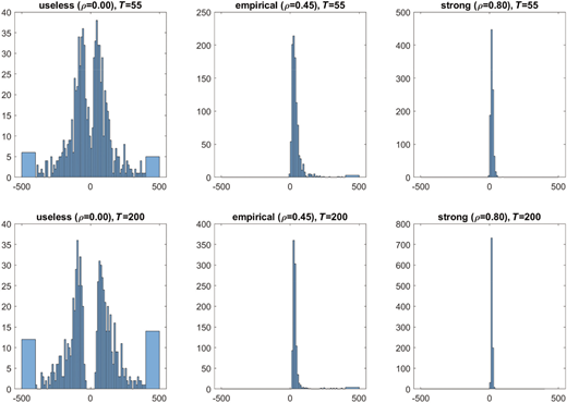
Monte Carlo Simulation: Distribution of GMM Point Estimates.
Monte Carlo Simulation: Distribution of GMM Point Estimates.
There is a shortcoming to using bootstrap confidence intervals from an econometric point of view. This method is not identification robust, as it is explained by Burnside (2011). If the factor is “useless,” the parameter of interest cannot be identified from the data. This means that the bootstrap confidence interval is uninformative about the parameter and does not tell us so directly. I believe that this is a minor issue in applied research in the case of consumption-based asset pricing. When results indicate that a factor is not priced with an economically reasonable coefficient of relative risk aversion, such an outcome is usually interpreted as evidence against the model. For example, in the case of reported consumption, it is well known that unreasonably large point estimates of the coefficient of relative risk aversion are required to fit the equity premium due to a lack of factor correlation. At least since Mehra and Prescott (1985), the usual conclusion taken from this finding is that the model does not explain the equity premium. They did not conclude that the model does a good job in explaining the equity premium but that investors have a large coefficient of relative risk aversion. This example illustrates that it is advisable to look at the test results in the context of economic theory and not confine the interpretation to a purely econometric perspective. Statistical inferences should go hand in hand with economicinference.5
Fama-MacBeth methodology and the linear model: In another set of results, Kleibergen and Zhan (2020) consider methods that evaluate whether a factor can help explain a cross-section of 31 portfolio excess returns using a linearized version of the consumption-based model. To this end, Kleibergen and Zhan (2020) propose replacing inference on the price of risk based on the standard Fama and MacBeth (1973)/Shanken (1992) methodology with the GRS-Factor Anderson-Rubin (GRS-FAR) test (which works analogous to the GMM-AR test).
I mainly criticize two aspects of their discussion: First, they overstate the “useless” factor problem in the context of the Fama-MacBeth/Shanken approach when the sample size is small. In line with Kan and Zhang (1999), I show that the “useless” factor problem is a large sample issue and not a small sample one. But the considered consumption factors are annually sampled and are a prime example of a small sample.
Second, if the asset pricing model is “misspecified” and cannot explain the data perfectly, the GRS-FAR test is expected to be unable to provide inference on the price of risk and cannot be expected to detect “useful” but imperfect factors (Figure 5). However, previous research has concluded that the model does not explain the data perfectly and is at best regarded as “misspecified” (Kroencke, 2017; Savov, 2011). Again, I argue that a test procedure that is robust against “useless” factors is not helpful for applied research if the test does not allow for the detection of “useful” factors.
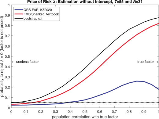
FMB/Shanken and GRS-FAR Power Curves With Varying the Risk Factor (Betas): Misspecified Model.
FMB/Shanken and GRS-FAR Power Curves With Varying the Risk Factor (Betas): Misspecified Model.
As before, an easy-to-implement alternative is to report bootstrap confidence intervals of the price of risk, as has been done by Burnside (2011). However, the same caveats described above regarding identification robustness apply.
What this paper is not about: This paper is not a general defense of the consumption-based asset pricing model and the alternative consumption measures. I do not think this is necessary. The alternative consumption measures are unlikely to explain all of the equity premium, and are unable to explain the cross-sectional dispersion in mean excess returns of many anomaly portfolios (e.g., Kroencke, 2017; Savov, 2011). The alternative consumption measures are also unable to capture the time-series variation in the price-dividend ratio (e.g., Kroencke, 2017, 2022). Recent survey-based evidence that has emerged at the investor level has been disappointing (Chinco et al., 2022; Choi and Robertson, 2020). But when we want to point out the weaknesses of the simple consumption-based model, we want do so based on powerful tests.
Outline: The outline of the paper is as follows. Section 1 describes the consumption-based model and the data, and offers a preliminary analysis that comes with a minimum of assumptions. Section 2 studies GMM-based inference for the nonlinear model, while Section 3 compares the Fama-MacBeth methodology with the proposed alternatives for the linearized version of the model. I conclude in Section 4. I skip a repetition of most of the formulas used for the econometric tests. These are provided in detail in the Online Appendix to Kroencke (2017) and the paper by Kleibergen and Zhan (2020).6
1 Model, Data, Preliminary Analysis
1.1 The Consumption-Based Model
The basic model: The central pricing equation in asset pricing is
where Mt+1 is the stochastic discount factor (SDF) and is an asset return in excess of the risk-free rate. A large part of the asset pricing literature tests how well different SDFs “fit” the pricing equation.
In the classic consumption-based asset pricing model, the non-linear SDF is7
where Ct+1/Ct = 1 + ΔCt+1 is consumption growth, δ is a time preference parameter that should be around one, and γ is the coefficient of relative risk aversion.8
A log-linearized version of the SDF is
In this equation, is de-meaned consumption growth.9Using the linearized SDF, the pricing equation can be re-formulated so that the expected excess return is on the left-hand side of the equation
The coefficient of relative risk aversion is not a free parameter. It describes investors’ willingness to take a risk. For risk-averse investors, this parameter must be strictly positive. It also cannot be arbitrarily large. As pointed out by Grossman and Shiller (1980) and Mehra and Prescott (1985), among many others, large values imply an implausibly large degree of risk aversion.10Grossman and Shiller (1980) consider values for γ up to 6 as plausible. Mehra and Prescott (1985) argue that γ = 10 is the highest level of risk aversion that can be considered as economically plausible. captures the riskiness of an asset. A large covariance suggests that the asset has low returns in bad times when consumption growth is also low (and marginal utility is high), for example, during recessions. Such an asset will have a low price and a high expected excess return, everything else being equal. It is probably this simple prediction that gives the model its appeal.
In empirical work, the return-beta representation is popular for testing
where βC is the consumption beta, and λ is the “price of risk.” is the same for all assets and is determined by investor preferences for risk (γ) and the amount of fundamental (non-diversifiable) risk in the economy .βC can vary between assets and is also called factor loading.
It is worth noting what the model does not predict. In particular, it does not predict that βC ≠ 0 holds for all assets. An asset with βC = 0 just earns a zero excess return (i.e., the risk-free rate): . Therefore, a test that indicates βC = 0 does not necessarily contradict the model or indicate a “useless” factor in the economic sense.11The model also does not predict a particularly large timeseries regression R2, as it describes a relationship between mean excess returns and consumption covariances. However, in line with Eq. (4), the time-series regression R2 should be distinct from zero if the mean excess return is different from zero.
The alternatives: The basic model is a strong simplification of the real world and it is reasonable to think about possible alternatives. A more realistic SDF might be written as
where f (st+1) captures a function over a vector of additional drivers (st+1) of the SDF. Setting ζ= 1 and ϕ= 0 nests the basic model. In fact, there is a rich and fruitful literature that provides evidence in favor of the existence of additional (or alternative) drivers of the SDF. Examples include Campbell and Cochrane (1999), Bansal and Yaron (2004), Yogo (2006), Piazzesi et al. (2007), Wachter (2013), Schreindorfer (2020), and many more, including models that incorporate investor heterogeneity, ambiguity, learning, institutional frictions, and outright irrationality.12
From an empirical point of view, consumption growth is already challenging to measure. But the potential other factors st+1 are arguably even more challenging to capture in an empirical analysis. Importantly, according to many advanced models, the consumption factor is not unrelated with the additional factors st+1. Often, f (st+1) captures some mechanism that amplifies basic consumption growth risk. For example, in the habit model of Campbell and Cochrane (1999), a slow-moving habit changes investors’ attitude toward risk. It can amplify the price reaction to large drops in dividends and consumption. Bansal et al. (2012) propose a calibration of the long-run risk model that requires a significant portion of “shortrun” consumption risk. A test of the basic model can also be interpreted as a “partial” test of a more advanced model.
For that reason, it is economically interesting to empirically test the basic model even if one does not think that it is literally true. Because a researcher can be almost sure that the model is misspecified, it might be better to write for asset i
where ai reflects an asset-specific component of the expected return that is not captured by short-run consumption risk. In empirical tests, this component should show up as a pricing error, a part of the mean excess return unexplained by the model. Accordingly, I argue that it is of utmost importance to use statistical methods that allow a researcher to draw reliable conclusions when the model is misspecified.
1.2 Some Preliminary Results
Table 1 reports some preliminary asset pricing results for the data used in Kroencke (2017) and Kleibergen and Zhan (2020). The consumption measures are the “reported” consumption from the NIPA accounts (Mehra and Prescott, 1985; Shiller, 1981), ultimate consumption (Parker and Julliard, 2005), fourth-quarter consumption (Jagannathan and Wang, 2007), “garbage” (Savov, 2011), and “unfiltered” consumption (Kroencke, 2017).13 Stock returns are sampled at the end of December (Dec.) or time-aggregated (T.A.) to account for the time-aggregation bias (e.g., Breeden et al., 1989; Cochrane, 1996; Kroencke, 2017). Details on the data sources and construction are provided in Kroencke (2017).
The Equity Premium and Alternative Consumption Measures.
| Short Sample (1960-2014) | Full Sample (1928-2014) | ||||||
|---|---|---|---|---|---|---|---|
| Reported Dec. | Garbage Dec. | P-J Dec. | Q4-Q4 Dec. | Unfiltered T.A. | Reported Dec. | Unfiltered T.A. | |
| Panel A: Identification | |||||||
| Covariance | 0.39 | 26.04 | 7.29 | 7.09 | 19.64 | 4.87 | 48.54 |
| Btrp c.i.95% | (−6.8,8.2) | (11.2,45.2) | (−7.6,24.8) | (−0.4,15.8) | (6.2,35.8) | (−7.0,17.4) | (24.5,79.4) |
| Correlation | 0.02 | 0.58 | 0.14 | 0.29 | 0.45 | 0.11 | 0.60 |
| Btrp c.i.95% | (−0.3,0.3) | (0.3,0.7) | (−0.2,0.4) | (−0.0,0.5) | (0.2,0.6) | (−0.2,0.4) | (0.4,0.7) |
| Beta | 0.23 | 3.21 | 0.72 | 3.32 | 2.95 | 1.03 | 3.00 |
| Btrp c.i.95% | (−3.2,3.6) | (1.9,4.5) | (−0.7,2.1) | (0.4,6.2) | (1.4,4.5) | (−0.9,2.9) | (2.2,3.9) |
| Panel B: Implied Economic Quantities | |||||||
| Rel. Risk Aversion, γ | 1,465.83 | 20.16 | 79.16 | 81.45 | 29.38 | 149.35 | 14.98 |
| Btrp c.i.95„% | (−2,598.8,2,365.5) | (1.8,70.2) | (−993.5,920.1) | (−424.2,807.7) | (4.6,123.2) | (−1,650.4,1,570.2) | (4.8,38.3) |
| Price of Risk, λ% | 25.07 | 1.63 | 8.07 | 1.74 | 1.96 | 7.07 | 2.42 |
| Btrp c.i.95„% | (−37.3,45.5) | (0.2,4.1) | (−89.7,99.0) | (−6.0,16.2) | (0.3,6.2) | (−71.3,63.8) | (1.0,4.4) |
| Equity Premium, % | 0.04 | 2.60 | 0.73 | 0.71 | 1.96 | 0.49 | 4.85 |
| Btrp c.i.95% | (−0.7,0.8) | (1.1,4.6) | (−0.7,2.4) | (−0.0,1.6) | (0.6,3.6) | (−0.7,1.7) | (2.4,8.0) |
Description: Panel A reports the covariance, correlation and beta of alternative consumption measures with the market excess return (T = 55, N = 1). Panel B shows the implied coefficient of relative risk aversion (γ) exploiting the linearized relationship. The price of risk is defined as λ = γ ∕Var(ΔCt). The implied equity premium imposes γ = 10, the maximum level of risk aversion considered plausible by Mehra and Prescott (1985). The dataset is the same as in Kroencke (2017) and Kleibergen and Zhan (2020); equity returns below Dec. (TA.) are measured at the end of December (Time-Aggregated). Bootstrap re-samples are used to determine 95% confidence intervals.
Interpretation: Reported consumption is insignificantly correlated with the market excess return (and might be regarded as a “useless” factor) and does not explain the equity premium; also known as the equity premium puzzle (Mehra and Prescott, 1985). Alternative consumption measures like garbage or unfiltered consumption have large and significant correlation coefficients and explain a part but not all of the equity premium. Estimated parameters (γ and λ) are later used to benchmark with other methods.
Panel A shows the covariances, correlation coefficients, and consumption betas in the post-war sample from 1960–2014. A significant factor correlation implies that the textbook methods allow to identify the coefficient of relative risk aversion or the price of risk. I use bootstrap re-sampling to compute 95% confidence intervals, similar to Savov (2011). The reported consumption measure has an insignificant consumption covariance of 0.0039%. On the other hand, the alternative consumption measures come with covariances in the range from 0.07 to 0.26%, and the covariances for unfiltered consumption and garbage are significantly different from zero. The overall conclusion does not change when considering the correlation coefficient or the beta. In the full sample, there are no data for garbage available. As pointed out in Kroencke (2017), an advantage of unfiltered consumption over garbage is that a longer time-period going back to 1928 is available. The full sample is studied in detail in Kroencke (2017) but is not considered by Kleibergen and Zhan (2020). In the full sample, the covariance is 0.49% for unfiltered consumption and is significantly different from zero.
Panel B provides some back-of-an-envelope calculations exploiting the approximate pricing (Eq. (4)). Following Campbell (2003), I divide the mean excess return of the market portfolio by the consumption covariance to get the implied coefficient of relative risk aversion. I use bootstrap re-sampling of this ratio to determine 95% confidence intervals. In the case of reported consumption, this leads to a division of 5.8% by something close to zero. Thus, the resulting coefficient of risk aversion is large and imprecisely measured as indicated by a large 95% confidence interval.
The same does not apply to the garbage measure or unfiltered consumption, which are significantly correlated with stock returns. For garbage (unfiltered consumption), the point estimate of the coefficient of relative risk aversion is 20 (29). The bootstrap confidence intervals are wide but indicate that is significantly different from zero for garbage and unfiltered consumption. In the full sample, unfiltered consumption gives a point estimate γ = 15, which comes with a relative tight 95% confidence interval of {5, 38}.
I also consider estimates of the price of risk λ based on Eq.(5). The results for reported consumption indicate that this consumption measure is not priced. Garbage gives a significant price of risk of 1.6% (95 c.i.: {0.2%, 4.1%}). Unfiltered consumption leads to a point estimate of about 2.0% (95 c.i.: {0.3%, 6.2%}).
For factors with insignificant factor correlation (e.g., reported consumption), it is not expected that the parameters λ and γ can be identified, because one might “divide by zero” in the absence of estimation errors. As a result, the bootstrap percentiles cannot be regarded as informative about the true parameter. Due to the lack of identification, the true parameter can have any value. As can be seen for reported consumption, a factor with lack of correlation is likely to come with an unreasonable large point estimate of γ and a very wide bootstrapped confidence interval, far away from the economically reasonable range (between zero and ten).
A simple solution to the “division by zero problem” of “useless” factors is not to divide. To this end, I impose an economically reasonable value for and then conduct inference on the expected excess return implied by the factor covariance multiplied with γ (Eq.(4)). This approach only requires multiplication and is comparable to the original Mehra and Prescott (1985) tests. In the bottom rows of Table 1, I impose γ = 10, the largest value considered plausible by Mehra and Prescott (1985), and I then ask how big the equity premium is given the consumption covariance. For reported consumption, the implied equity premium is a meager four basis points and is insignificant. Garbage, by contrast, can explain a significant amount of 2.60% (95 c.i.: {1.1%, 4.6%}) of the equity premium. Unfiltered consumption can explain 1.96% (95 c.i.: {0.6%, 3.6%}). Thus, in the most optimistic case ( γ = 10), the alternative consumption measures explain around 44% (2.6/5.8) and 33% (1.9/5.8) of the equity premium in the short sample. The full sample point estimates indicate a somewhat larger share of 66% (4.8/7.3) explained by unfiltered consumption. A zero consumption-based equity premium can be rejected according to the 95% confidence interval.
To sum up, this section illustrates that alternative consumption measures and the market excess return are statistically significantly correlated. These correlations are economically relevant and imply that alternative consumption measures can explain part of the equity premium. However, this correlation is not large enough to fully explain the equity premium with an economically reasonable coefficient of relative risk aversion. The results also do not rule out alternative models (e.g., when consumption growth happens to correlate with alternative drivers of the SDF). At best, the consumption-based model is misspecified. In the remainder of the paper, I show that powerful tests confirm the preliminary results reported in Table 1.
2 GMM Estimation and the Non-Linear Model
2.1 Moment Conditions
It is common in the literature to test the non-linear version of the classic consumption-based asset pricing model as stated in Eq.(2). The GMM approach allows to estimate the parameters of interest (δ, γ) by exploiting the pricing equation for N test asset excess returns,. Accordingly, the GMM objective function is
where W is a N N weighting matrix and are 1 × N moment conditions
Because the time preference parameter does not affect the equity premium, Savov (2011) and Kroencke (2017) fix this parameter to δ = 0.95.14Thus, there is only one parameter to be estimated, and a single moment condition is sufficient to estimate . It is common in the literature to use the market excess return as the only test asset (N = 1) to obtain a baseline estimate. In the following, I focus the discussion on this case.
The weighting matrix: As discussed in detail by Cochrane (2005), a different weighting matrix W might be preferred in different situations, but it should be picked with care. Kroencke (2017) uses W = 1. Kleibergen and Zhan (2020) prefer W = Ŝ−1, where15
Using W = 1 (in the case of one moment condition) means that the GMM objective function compares how different γ reduce the “pricing error” measured by gT. In contrast, gTŜ−1g'T, compares the impact of different γ on the ratio of the squared pricing error to its variance. The second specification comes with one potential disadvantage. Specific parameter values of γ might blow up estimates of S rather than reducing gT, as Cochrane (2005, p. 279), warns. When the estimation is conducted with only one moment condition, the specification W = Ŝ−1 loses its potential advantage to utilize the available moment conditions efficiently.
I show both objective functions for unfiltered consumption on the left-hand side of Figure 2. The objective function studied in Kroencke (2017) is steep for large absolute values of γ, indicating large pricing errors, while the objective function of Kleibergen and Zhan (2020) is flat and even slightly decreasing. This must come from S increasing even faster than the pricing errors (this is the only difference between the two curves). Now, looking at the moment condition, it is apparent that this is a power function of γ. Thus, it might not be surprising that S(γ) eventually is a very large number for large enough values of. In fact, I find that for example at γ = −5092 , Ŝ is computed to be infinity in the statistical software package used, which leads to, even though gT is a pricing error as large as 1.16e+153 (in words, around one quinquagintillion). This is a race of a large pricing error versus a large S, where S eventually wins.16As a result, the objective function of Kleibergen and Zhan (2020) has multiple minima, one reported at 22.5, as well as several others for γ s somewhere around −5,000 and +7,000. In the following, I refer to such a GMM objective function as an “ill-conditioned” GMM objective function.
The J-test: The J-test is a test of whether the moment conditions are jointly equal to zero, in general · The same test statistic can be used for both specifications for the weighting matrix W = 1 and W = Ŝ−1, as it can be verified using the formulas provided by Cochrane (2005), p. 255.17
2.2 The GMM-Rank Test
If the factor and the test asset return are uncorrelated, it is not possible to identify the parameter of interest (γ). Asymptotic inference is derived under the assumption that there is factor correlation, which can lead to an over-rejection of the hypothesis that the factor is not priced, that is, the H0: γ = 0.
Savov (2011) shows that the correlation between garbage and stock returns is economically large, about 0.58 (he reports a bootstrapped standard error of 0.11). Kroencke (2017) finds a similarly large correlation for unfiltered consumption. Table 1 shows that these correlation coefficients are highly statistically significant. Nevertheless, Kleibergen and Zhan (2020) are concerned about an insufficient correlation between consumption and stock returns such that cannot be identified and GMM standard errors cannot be trusted.
To provide evidence for their claim of insufficient factor correlation, Kleibergen and Zhan (2020) report a test of the first derivative of the moment condition
where Δct+1 is log-consumption growth. The GMM-rank condition is that hT ≠ 0. Rejection of the H0: hT = 0 would indicate that there is sufficient factor correlation, which suggests that the usual GMM-based inference is reliable. But for hypothesis testing, they re-estimate γ using the moment function of the rank condition. They do not simply use the GMM estimates coming from gTŜ−1 g'T, but rely on a new J-test that is based on hTŜ−1h'T.
I plot this new objective function on the right-hand side of Figure 2. I find that this GMM estimate is certain to fall into the “GMM trap.” There is always a solution for γ around −5,000 and +7,000 because S is computed to be infinity at some point. The problem renders the GMM-rank test meaningless, because there are only corner solutions for this objective function and no (local) minimum is even close to the economically reasonable region or the initial GMM estimate. Because the objective function divides by infinity at the corner solutions, the test of H0: hT = 0 cannot reject. The problem is not an insufficient correlation but an ill-conditioned GMM objective function.
Size and power of the GMM-rank test: I illustrate the implications for empirical work in Figure 1. I run a Monte Carlo simulation that imposes normal and i.i.d. returns and consumption growth to generate 10,000 samples with T = 55 (results for T = 200 are reported in the Appendix).18I calibrate the simulation to the market excess return and unfiltered consumption, except that I vary the population correlation coefficient between zero (the “useless” factor) and 1.00 (the “most useful” factor one can hope for), which is reported on the x -axis. Unfiltered consumption and garbage correspond to the middle area of the figure (correlation between 0.40 and 0.60). The y-axis shows the percentage of the simulations where I can reject the hypothesis that there is no factor correlation (more precisely, the H0: hT = 0).
I consider three different tests: (i) the GMM-rank test, as reported in Kleibergen and Zhan (2020), with the ill-conditioned GMM objective function, (ii) a modified version of the GMM-rank test that imposes the identity matrix (i.e., W = 1), such that the GMM objective function is well-behaved (see Figure 2), and (iii) a direct test of the hypothesis that the correlation coefficient is equal to zero (similar to Savov, 2011).19 which is likely to increase the small sample power of the test.
Figure 1 shows that the probability to reject the GMM-rank test is virtually zero no matter how large the correlation with the market factor is. The rank test as conducted by Kleibergen and Zhan (2020) does not allow one to make a meaningful conclusion about the rank condition. The corrected GMM-rank test proposed in this paper has the power to detect “useful” factors. However, I find that a direct test of the correlation coefficient is considerably more powerful in small samples.
To sum up, the GMM-rank condition does not fail because of insufficient factor correlation, as claimed by Kleibergen and Zhan (2020).20The rank condition fails because the GMM objective function used by Kleibergen and Zhan (2020) is numerically ill-conditioned.
2.3 The GMM-AR Test
I now turn to GMM-based inference on the coefficient of relative risk aversion. I run a Monte Carlo simulation that imposes normal and i.i.d. returns and consumption growth to generate 1,000 samples with T = 55. As before, I vary the population correlation coefficient between zero (the “useless” factor) and 1.00, which is reported on the x -axis. I then count the fraction of simulations in which asymptotic GMM standard errors indicate that the coefficient of relative risk aversion is estimated to be significant at the 5% level.21
Figure 3 shows the probability of finding a significant coefficient of relative risk aversion. For a useless factor, is not identified and this probability should not exceed 5%. As can be seen, the GMM-based standard errors over-reject the “useless” factors.
To avoid this issue, Kleibergen and Zhan (2020) propose using the GMM-AR test instead of the GMM-based standard errors. To this end, they calculate the p-value for the test H0: JT = 0 at various hypothesized values γ = γ0. The 100 × (1 − 0.05)% confidence set for γ then contains the bounds where JT = 0 cannot be rejected. The confidence set is unbounded when JT is insignificant at the entire set of possible values of γ. It is disjointed when the confidence set is open from one side. The confidence set is empty when JT is always significantly different from zero. It is not possible to conduct inference on γ when the confidence interval is unbounded, disjointed or empty. Accordingly, these cases count in the simulation as “the H0: γ = 0 is not rejected.”
The GMM-AR test is robust to “useless” factors, as can be seen in Figure 3. However, I find that the GMM-AR test has a low power to detect “useful” factors. For example, a hypothetical factor with a population correlation coefficient of 0.90 would be detected with a probability of less than 30%. For a factor with an economically large correlation coefficient of 0.50, the probability is 5%.
3.4 GMM Bootstrap Confidence Intervals
An alternative to the GMM-AR test is to conduct a pairwise bootstrap and to report the confidence interval of the bootstrapped GMM estimates of the coefficient of relative risk aversion. Figure 3 illustrates that such bootstrap confidence intervals do not over-reject “useless” factors and, at the same time, remain powerful for detecting “useful” factors.
To illustrate why bootstrap confidence intervals do not over-reject, I report in Figure 4 the distribution of GMM estimates from the Monte Carlo simulation for selected population correlation coefficients. For the “useless” factor, the distribution is centered around zero and is non-standard. When I consider the simulation results with increased time-series observations (T = 200), the distribution becomes even wider instead of narrower, which shows that it is not possible to identify the parameter. Intuitively, sample covariances are closer to zero in the larger sample, resulting in more γ estimates that are further from zero. However, the bootstrap confidence interval will take the non-standard shape and the width of the distribution into account and, therefore, avoids an over-rejection problem. From the figure, it is clear that bootstrap standard errors (or t-statistics) do not work, as they require a distributional assumption. For the linear version of the model, Burnside (2011) provides bootstrap confidence intervals in his analysis to mitigate the risk of over-rejecting “useless” factors. He stresses that the bootstrap confidence interval is not identification robust. From the confidence intervals alone, a researcher cannot infer that a factor is “useless” and the parameter cannot be identified, or that the true parameter is around zero.22
3.5 Empirical Results Revisited
The non-linear model: In Table 2, I show the GMM results for the short sample (as in Kleibergen and Zhan, 2020) and the full sample (not shown in Kleibergen and Zhan, 2020). The reported consumption measure requires an unreasonably large coefficient of relative risk aversion of 137 and is not able to set the single moment condition (the pricing error) to zero (JT = 0.85). While the estimate for is significant, the unreasonably large point estimate and the non-zero pricing error allow to conclude that reported consumption has no explanatory power for the equity premium (e.g., Kroencke, 2017; Mehra and Prescott, 1985; Savov, 2011). The garbage measure allows for an estimate of the coefficient of relative risk aversion of 16. Unfiltered consumption provides an estimate of 23. Both estimates are significant at the 10% level based on GMM standard errors. These two estimates also come close to the economically reasonable range between zero and ten. All of the alternative consumption measures allow to set the single moment condition to zero (JT = 0.00). In the full sample, unfiltered consumption provides an estimate of 10, which is significant at the 5% level.
GMM Estimates for the Coefficient of Relative Risk Aversion: Non-Linear Model.
| Short Sample (1960–2014) | Full Sample (1928–2014) | ||||||
|---|---|---|---|---|---|---|---|
| T = 55 and N = 1 | T = 87 and N = 1 | ||||||
| Reported Dec. | Garbage Dec. | P-J Dec. | Q4-Q4 Dec. | Unfiltered T.A. | Reported Dec. | Unfiltered T.A. | |
| γ | 137.14 | 15.63 | 42.35 | 64.05 | 22.53 | 36.86 | 10.32 |
| se(γ) | 52.82 | 8.30 | 23.60 | 40.41 | 12.13 | 13.36 | 4.55 |
| Btrp c.1.9m | (−2,806.2,1,030.9) | (1.5,92.7) | (−1,185.6,1,644.7) | (7.6,1,798.9) | (2.8,131.6) | (-181.5,592.9) | (4.3,206.3) |
| GMM-AR c.i.950∕0 | unb./disjointed | unb./disjointed | unb./disjointed | unb./disjointed | unb./disjointed | unb./disjointed | unb./disjointed |
| JT | 0.85 | 0.00 | 0.00 | 0.00 | 0.00 | 0.00 | 0.00 |
| p(rank), KZ | 1.00 | 0.29 | 0.29 | 0.50 | 0.29 | 0.30 | 0.31 |
| p(rank), corrected | 1.00 | 0.00 | 0.14 | 0.14 | 0.00 | 0.00 | 0.00 |
| p(corr) | 0.90 | 0.00 | 0.32 | 0.03 | 0.00 | 0.30 | 0.00 |
Description: This table shows estimates of the coefficient of relative risk aversion (γ) using the non-linear GMM moment condition:
The market excess return is the single test asset. Below the GMM estimate of γ is the GMM standard error, and the 95% confidence interval of γ according to a pairwise bootstrap or the GMM-AR test. JT is the value of the objective function, p(rαnk), KZ, is the p-value to the GMM-rank test as in Kleibergen and Zhan (2020), which leads to an ill-conditioned objective function (Figure 2). p(rαnk), corrected, is the p-value for an alternative version of the GMM-rank test where the objective function is well-behaved (also shown in Figure 2). p(cor), is the p-value for a direct test of the correlation coefficient. The short sample is considered by Kleibergen and Zhan (2020) but not the full sample period.
Interpretation: According to the GMM-rank test, as implemented by Kleibergen and Zhan (2020), no consumption factor is significantly correlated with the market excess return. The unbounded/disjointed GMM-AR confidence intervals do not allow to conclude that consumption has explanatory power for the equity premium. However, the direct test of the correlation coefficient indicates that garbage, Q4-Q4, and unfiltered consumption are significandy correlated with the market excess return. The bootstrap confidence intervals do not include zero and indicate that garbage, Q4-Q4 and unfiltered consumption help to explain the equity premium.
The difference in the test outcomes are in line with the power curves shown in Figures 1 and 3. The GMM-AR and the GMM-rank tests suffer from the “GMM trap” problem and have low or no power to detect “useful” factors. The modified GMM-rank test, or testing the correlation coefficient directly, is considerably more powerful in detecting “useful” factors (Figure 1). Bootstrap confidence intervals do not over-reject “useless” factors and are powerful in detecting “useful” factors (Figure 3). Kleibergen and Zhan (2020) attribute the difference between GMM-AR test and GMM standard errors to an incorrect size of the textbook approach in the presence of a “useless” factor. Except for reported consumption, the extended results in this paper show that the difference in the two tests can be attributed to the low power of the GMM-AR test.
In contrast, the GMM-AR test is for all specifications unbounded/disjointed. Kleibergen and Zhan (2020) argue that the unbounded GMM-AR test is symptomatic of insufficient factor correlation for all of the considered consumption measures. To provide evidence for this claim, they report the p-value of the GMM-rank test (p(r ank), KZ), which indeed does not allow one to reject the null hypothesis of insufficient factor correlation.
However, as shown in Figure 1, this GMM-rank test has no power to detect “useful” factors and will also indicate insufficient correlation for a perfectly correlated factor. A similar issue plagues the GMM-AR test (Figure 3). When I impose the identity matrix for the GMM-rank test, the test is well-behaved and powerful (Figure 1). In the table, I find that garbage and unfiltered consumption have p-values below 0.05 and pass the “corrected” version of the GMM-rank test. The direct test of factor correlations (p(corr)) corroborates this conclusion; the Q4-Q4 measure now also passes. This suggests that traditional GMM-based inference is actually trustworthy when using alternative measures of consumption.
In Table 2, I also report 95% bootstrap confidence intervals for . As shown in Figure 3, the bootstrap confidence intervals do not over-reject “useless” factors and are powerful for detecting “useful” factors. They are large and include the value of zero for the consumption measures that fail the simple factor correlation test (e.g., reported consumption), and they do not include zero for the consumption measures that pass this direct test for sufficient factor correlation (garbage, Q4-Q4, and unfiltered consumption).
The linearized model: If a researcher still wants to perform the GMM-AR test for consumption-based asset pricing, a potential solution could be to consider the linearized version of the model (Eq.(4)), which means that we are back to the model analyzed in Section 1. Because this function is linear in γ, it is less likely that S will grow faster than the pricing error. In addition, the GMM-rank test of this specification has the desirable economic interpretation of testing directly consumption covariances, H0: which is also invariant of . Rejection of this hypothesis indicates that factor correlation is sufficient and that GMM standard errors are reliable.
The results are reported in Table 3. I find that the same consumption measures that pass the more powerful rank tests in Table 2 now also pass the rank test of the linear model. The GMM-AR test also leads to a bounded confidence set in these cases and indicates that consumption is priced. Point estimates are similar to Table 1. Bootstrap confidence intervals are somewhat tighter compared to the GMM-AR counterparts but allow for the same conclusions in this application.
GMM Estimates for the Coefficient of Relative Risk Aversion: Linearized Model.
| Short Sample (1960–2014) | Full Sample (1928γ2014) | ||||||
|---|---|---|---|---|---|---|---|
| T = 55 and N = 1 | T = 87 and N = 1 | ||||||
| Reported Dec. | Garbage Dec. | P-J Dec. | Q4-Q4 Dec. | Unfiltered T.A. | Reported Dec. | Unfiltered T.A. | |
| γ | 1,465.83 | 20.16 | 79.16 | 81.45 | 29.38 | 149.35 | 14.98 |
| se(γ) | 10,010.85 | 13.09 | 89.35 | 59.62 | 20.36 | 192.99 | 8.38 |
| Btrp c.i.95% | (−350.3,2,784,373.2) | (3.6,81.2) | (−103.6,1,687,182.3) | (12.7,958.1) | (4.6,142.3) | (−415.5,2,032,094.4) | (4.4,47.8) |
| GMM-AR c.i.95o∕0 | unb./disjointed | (4.4, 115.9) | unb./disjointed | (18.3, 4359.1) | (4.9, 201.6) | unb./disjointed | (4.4, 66.0) |
| JT | 0.00 | 0.00 | 0.00 | 0.00 | 0.00 | 0.00 | 0.00 |
| p(rank) | 0.88 | 0.01 | 0.28 | 0.04 | 0.01 | 0.38 | 0.01 |
| p(corr) | 0.90 | 0.00 | 0.32 | 0.03 | 0.00 | 0.30 | 0.00 |
Description: This table shows estimates of the coefficient of relative risk aversion (γ) using the linear GMM moment condition:
The market excess return is the single test asset. Below the GMM estimate of γ is the GMM standard error, and the 95% confidence interval of γ according to a pairwise bootstrap or the GMM-AR test. JT is the value of the objective function, p(rαnk), is the p-value for the GMM-rank test which is equivalent to test the hypothesis HO:, is the p-value for a direct test of the correlation coefficient.
Interpretation: A linearized version of the model is robust to the “GMM trap” problem. Now both the bootstrap and GMM-AR confidence intervals allow for the same conclusion that garbage, Q4-Q4 and unfiltered consumption help to explain the equity premium. GMM standard errors require testing at a higher significance level to come to the same conclusion.
The benefit of the GMM-AR test is that unbounded/disjointed confidence intervals directly indicate a lack of identification. The economically reasonable range is often described as being from zero to ten (Mehra and Prescott, 1985). Against this backdrop, a bootstrap confidence interval of {−350, 2,784,373} for reported consumption is, in practical terms, very much the same thing as an unbounded/disjointed confidence interval.
Summary of GMM estimates: The GMM-rank test and the GMM-AR test as they are implemented in Kleibergen and Zhan (2020) are not in line with the general idea of providing robust inference. Both suffer from the GMM trap and are inconclusive even when factor correlation is strong. If low factor correlation is a concern, it is more useful to test the factor correlation directly and to rely on GMM standard errors. A reliable alternative is to report bootstrap confidence intervals.
3 The Fama-MacBeth Method and the Linearized Model
Kleibergen and Zhan (2020) also consider methods to test linear cross-sectional asset pricing models (Eq.(5)) for a large cross-section of stock returns (N = 31). In this context, I mainly criticize two points: First, they overstate the “useless” factor problem of the Fama-MacBeth/Shanken methodology. In particular, they claim that the textbook approach cannot be trusted and suffers from a “malfunction,” such that a researcher is likely to over-reject the hypothesis that a “useless” factor cannot price a cross-section of stock returns. I show that this claim is false and that a researcher will not over-reject a “useless” factor if the sample size is small, as in their empirical application. The over-rejection problem of “useless” factors is a large sample problem and not a small sample one, as it is also stated in the classic study by Kan and Zhang (1999).
Second, the proposed alternative procedure, the GRS-FAR test, is not useful for inference on the price of risk (λ) when a model is misspecified. In this case, the expected confidence interval is “empty” and it is not possible to reject the H0:λ= 0. The problem is not a numerical issue, as for the GMM-based tests, but simply that the GRS-FAR test is expected to be unable to provide inference on the price of risk when the model is misspecified.23From the discussion provided by Kleibergen and Zhan (2020), I think it is possible (but not straightforward) to see that the GRS-FAR test cannot be expected to allow for inference on the price of risk for misspecified models.24Importantly, Kleibergen and Zhan (2020) claim that the GRS-FAR test is appealing for inference on the price of risk in consumption-based asset pricing. I disagree because this claim does not recognize that the literature regards the consumption-based asset pricing models as misspecified (Kroencke, 2017; Savov, 2011).
Moreover, a better alternative is available for testing the linearized model. As shown in a more general setting by Kroencke and Thimme (2020), bootstrap confidence intervals (as applied by Burnside, 2011) are robust to the “useless” factor problem independently of the sample size and even account for model misspecification. Moreover, Kroencke and Thimme (2020) show that the bootstrap confidence intervals are more powerful compared to a wide range of other methods that have been proposed in the literature.
3.1 Cross-Sectional Estimation of the Price of Risk
Here, I provide a brief review of the Fama-MacBeth/Shanken methodology and the GRS-FAR test.25
The Fama-MacBeth Shanken: This methodology provides a simple way to estimate the price of risk (λ) in the expected excess return-beta relationship
It rests on the following three steps:
Estimate the factor betas (βC,i) using time-series regressions for the i = 1, . . . ,N test asset returns that are tested.
Run a cross-sectional regression of the sample means of the excess returns of the N test assets on the N estimated factor betas to get an estimate of the price of risk λ.
Compute Shanken (1992)-standard errors for λ that account for the betas being estimated in the first step.26
A popular alternative is to estimate the model with a cross-sectional intercept (λ0) which can be interpreted as a “common” pricing error
In this case, the common pricing error (λ0) is the part of the expected return not explained by the model (e.g., Burnside, 2011). An economic argument can be, for example, that the subtracted risk-free rate includes a safety/liquidity premium, and λ0 allows one to account for this.27 Statistically, the additional degree of freedom (λ0) makes it easier to fit mean returns in the data. But it also means that an additional parameter needs to be identified from the data, which can reduce the power of empirical tests in small samples (see Kroencke and Thimme, 2020 for a detailed analysis).
GRS-FAR test: The GRS-FAR test proposed by Kleibergen and Zhan (2020) can be implemented according to the following steps:
De-mean the risk factor and add back a hypothesized price of risk.
Estimate the factor alphas (ai, or pricing errors) using time-series regressions for the i = 1, . . . ,N test asset returns using the modified risk factor.
Compute the GRS-test (Gibbons et al., 1989) on the joint significance of the N alphas.
Repeat the steps one to three for a wide range of values for the hypothesized price of risk.
The GRS-FAR confidence set is the region of the price of risk where the GRS-test does not reject that the alphas are jointly significantly different from zero at a given significance level.
Kleibergen and Zhan (2020) show how to adapt the GRS-FAR test to a test with a common pricing error (λ0).
The GRS-FAR test produces bounded confidence sets when there is a single region where the pricing errors are insignificant according to the GRS-test. In this scenario, it is possible to conduct inference on the price of risk (λ). The confidence set is unbounded when the pricing errors are insignificant at the entire set of possible values of the price of risk. It is disjointed when the confidence set is open from one side. The confidence set is empty when the pricing errors are always significant. It is not possible to conduct inference on the price of risk when the confidence interval is unbounded/disjointed or empty.
With increasing sample size, the power of the GRS-test will increase. The implication for applied research is that only a correctly specified model (all assets have a population pricing error of exactly zero) is expected to provide a bounded confidence interval in a large enough sample. If the model is misspecified (at least one single pricing error is non-zero), the expected result from the GRS-FAR test is an empty confidence interval. In other words, with an increasing sample size, the GRS-FAR test is expected to allow for inference on the price of risk only if the model is expected to explain all mean excess returns perfectly.
3.2 Are Fama-MacBeth Estimates “Trustworthy”?
Kleibergen and Zhan (2020) state that they are worried about inference based on Fama-MacBeth regressions in the usually rather small samples observed in consumption-based asset pricing. They mainly refer to the earlier literature, in particular the studies by Kan and Zhang (1999) and Kleibergen (2009) to motivate their worries.28 Surprisingly, I cannot find evidence in this literature that Fama-MacBeth regressions cannot be trusted in small samples. Kan and Zhang (1999) show that Fama-MacBeth regressions over-reject “useless” factors in (very) large samples. But they also show that Fama-MacBeth regressions under-reject “useless” factors in small samples, which is the relevant case in consumption-based asset pricing when T = 55. The over-rejection problem of “useless” factors is a large sample problem and not a small sample problem.
The evidence provided in Kleibergen and Zhan (2020) is based on power curves that can be also found in Kleibergen (2009). However, these power curves vary the price of risk (λ) and not the population factor betas (i.e., the population correlation coefficients). By construction, these power curves do not include the “useless” factor case where the population correlation coefficients are exactly zero. In the Appendix, I report the results of a replication and extension of this type of analysis. I find that the Kleibergen and Zhan (2020) power curves for unfiltered consumption actually indicate no problem with the Fama-MacBeth approach.
Moreover, when I construct power curves that take empirically relevant cases of misspecified models into account, the traditional Fama-MacBeth approach is arguably more “trustworthy” in small samples than the GRS-FAR test.
3.2.1 Power Curves with a “Useless” Factor
In this section, I fill this gap and study the properties of the Fama-MacBeth method and alternatives when a “useless” factor is actually present. To this end, I closely follow (and extend) the simulation design conducted by Kan and Zhang (1999). In line with Kan and Zhang (1999) and Kleibergen and Zhan (2020), I use a Monte Carlo simulation that imposes normal and i.i.d. returns and consumption growth to generate 10,000 samples. I consider the short sample period with T = 55 and N = 31 test assets. The true factor imposes the sample correlation of unfiltered consumption as the population correlation, Ft,true. In order to study a misspecified model, I impose the sample pricing errors of unfiltered consumption as the population pricing errors in the simulation. The “useless” factor has the same mean and standard deviation as unfiltered consumption, but I impose a zero correlation on all stock returns, Ft,useless . To construct a power curve, I form a portfolio of the “useless” factor (Ft,useless) and the true factor (Ft,true) and determine the correlation to the true factor using the equation
where ρ is the population correlation coefficient of the “measured” factor Ft with the true factor. I then use the Fama-MacBeth methodology with Shanken standard errors and the GRS-FAR confidence intervals to test the hypothesis that the price of risk (λ) is zero, H0: λ= 0, at the 5% significance level. Estimation is without
an intercept.29 I then count how often I can reject the null hypothesis across the 10,000 samples.
The results for ρ = 0 match with the simulation experiment by Kan and Zhang (1999). The results for ρ > 0 extend the analysis by Kan and Zhang (1999) and illustrate how powerful a method is in detecting “useful” factors that vary in their correlation to the test assets. For ρ = 1.0, the population properties of the factor are equal to the sample estimates of unfiltered consumption.
Figure 5 summarizes the results. Similar to Kan and Zhang (1999), I find that the Fama-MacBeth/Shanken standard errors do not over-reject “useless” factors ( x -axis: ρ = 0) in the small sample with T = 55 years. For the empirical factor ( x -axis: ρ = 1.0), the Fama-MacBeth/Shanken methodology finds a significant price of risk in about 80% of the simulations and is relatively powerful. The GRS-FAR test does not “over-reject” useless factors. However, this test has an almost flat power curve for misspecified models and usually does not detect a factor that helps to explain some of the mean returns.
The results presented apply to the considered set of test assets, the sample size, and the estimation without an intercept. For a different set of test assets, when the sample size is larger, or when the estimation is with an intercept, the Fama-MacBeth approach might over-reject “useless” factors. Examples are provided in the Appendix. For this reason, it is generally advisable to consider a method which is robust to the “useless” factors problem.
Bootstrap confidence intervals:Kroencke and Thimme (2020) provide a comprehensive comparison of various alternative “robust” approaches for cross-sectional asset pricing tests of linear models. A method that stands out is the pairwise bootstrap confidence interval, as reported by Burnside (2011). The bootstrap confidence interval does not over-reject “useless” factors. At the same time, this method accounts for model misspecification and is powerful in detecting “useful” factors. For this reason, I also report results for the bootstrap confidence interval for consumption-based asset pricing in Figure 5. The bootstrap confidence interval has the correct size and is powerful in detecting “useful” consumption factors. In the Appendix, I show that this is also the case when the Fama-MacBeth approach is not size correct, for example, in large samples.
Mirroring the discussion for GMM above, the bootstrap confidence interval comes with the disadvantage that this is not an identification robust method, as explained by Burnside (2011). When the factor is useless, the confidence interval will not indicate that the price of risk is around zero but rather that the price of risk cannot be identified from the data. I cannot see that this is a major problem in consumption-based asset pricing. An insignificant price of risk is usually interpreted as evidence against the model and is, therefore, not used for inference on the “true” price of risk.
3.3 Rank Tests, Univariate Factor Tests, and Tests of Mean Returns
Kleibergen and Zhan (2020) propose pre-testing risk factors to gauge whether the Fama-MacBeth/Shanken method is expected to provide valid inference. However, the proposed rank tests are not necessarily powerful in detecting useful factors in small samples when N is close to T . Testing with both a larger T and a smaller N can help improve power. In addition, the required normal-i.i.d. assumption is violated in the empirical data and the test is potentially inaccurate. I propose to apply a rank plausibility test on a shrunken cross-section with N = 1.
3.3.1 Multivariate Rank Tests
Inference based on the Fama-MacBeth method can be expected to be valid when the factor betas of the test assets are in the population different from zero (estimation without constant) or different from each other (estimation with a constant). Multivariate asymptotic Wald-tests, which are heteroskedasticity and autocor-
relation robust, are straightforward to conduct but are prone to over-rejection when T is small, and N is relatively large, as pointed out by Kleibergen and Zhan (2020).30To avoid this problem, Kleibergen and Zhan (2020) propose conducting a finite sample F-test that requires the data to be normal-i.i.d. They show that the F-test does not over-reject “useless” factors when N is close to T . But they do not investigate the power to detect useful factors (particularly when the normal-i.i.d. assumption is violated).
3.3.2 Univariate Factor Tests as a Rank Plausibility Test
The empirical data are not normal-i.i.d. and in such a setting a multivariate F-test is not necessarily powerful for detecting “useful” factors when N is close to T.31For this reason, I propose a simple rank plausibility test. More specifically, I shrink the cross-section to two portfolios formed on the test assets mirroring the two respective F-tests suggested by Kleibergen and Zhan (2020). The first portfolio invests equally in all (“ALL”) test assets, RALL,t . Motivated by financial theory, I use a t-test of the hypothesis that the beta of the “ALL” portfolio is significantly larger than zero
The beta of this portfolio is equal to the average of the betas of the test assets. A significant beta of the “ALL” portfolio suggests that there should be sufficient covariation in the cross-section to determine the price of risk in Fama-MacBeth regressions that impose a zero intercept.32
The second portfolio constructs a standard Fama and French (1993) high-minus-low (“HML”) portfolio based on the characteristics of the test assets. It goes long in the 50% of test assets that are predicted by a lagged characteristic to have a high mean return and short in the 50% of the test assets that are predicted by a lagged characteristic to have a low mean return.33Once again, motivated by finance theory, I use a t-test of the hypothesis that the beta of the “HML” portfolio is significantly larger than zero
The beta of this portfolio can be used to test whether there is a spread in betas that lines up with predicted mean excess returns. For univariate testing, it is far more likely that I can rely on asymptotic but heteroskedasticity robust (HC), or heteroskedasticity robust and autocorrelation (HAC) robust tests even when T is small.
While the univariate tests do not replace rank tests in the econometric sense, they help to detect cases where the F-test is inaccurate and/or has low power (e.g., because the normal-i.i.d. assumption is invalid, or when the inverse of the variance-covariance matrix is numerically inaccurate when N is close to T). For example, if the multivariate rank tests do not indicate sufficient factor betas, but the univariate tests do indicate sufficient factor betas, a researcher might want to reduce N (or increase T) to elevate the power of the multivariate test.
On the other hand, if the multivariate rank tests indicate sufficient factor betas but the univariate tests do not line up, it might indicate that just a few test assets drive the multivariate test result. Such a finding would suggest that the conclusions based on the Fama-MacBeth/Shanken methodology are technically valid (the price of risk can be econometrically identified), but that the estimate of the price of risk is not “robust” if some test assets are excluded from the analysis. A researcher can avoid such a pitfall by also reporting the individual betas of all test assets. If the goal is to conduct robust inference, the multivariate rank test should not be used as a substitute for an analysis of individual betas (or correlations).
3.4 Empirical Results Revisited
3.4.1 Baseline Results
Table 4 provides Fama-MacBeth estimates of the price of risk (λ) when the intercept is restricted to zero.34The Fama-MacBeth method is not generally well-behaved,even though it is unlikely to over-reject in small samples. For this reason, I add bootstrap confidence intervals (Burnside, 2011) as they do not over-reject “useless” factors in more general cases (see Kroencke and Thimme, 2020). Finally, I report the GRS-FAR confidence intervals as proposed by Kleibergen and Zhan (2020).
Price of Risk Estimates: Estimation Without Intercept.
| Short Sample (1960–2014) | Full Sample (1928–2014) | ||||||
|---|---|---|---|---|---|---|---|
| T = 55 and N = 31 | T = 87 and N = 21 | ||||||
| Reported Dec. | Garbage Dec. | P-J Dec. | Q4-Q4 Dec. | Unfiltered T.A. | Reported Dec. | Unfiltered T.A. | |
| λ | 0.31 | 2.09 | 10.14 | 2.28 | 2.44 | 7.87 | 2.66 |
| t(λ)sh | 0.57 | 2.51 | 1.05 | 1.87 | 2.59 | 1.00 | 3.32 |
| Btrp c.i.95% | (−4.8,4.9) | (0.6,4.6) | (−10.8,13.6) | (−1.8,5.4) | (0.9,5.4) | (-9.2,9.3) | (1.2,4.3) |
| GRS-FAR c.i.95% | unbounded | (−0.8, 7.8) | unbounded | unbounded | disjointed | empty | (0.9, 5.5) |
| implied γ | 17.64 | 25.25 | 97.75 | 104.84 | 35.95 | 164.24 | 16.26 |
| # signif. positive | 0 | 31 | 0 | 25 | 31 | 1 | 21 |
| t(βALL) p-value | 0.50 | 0.00 | 0.21 | 0.04 | 0.00 | 0.28 | 0.00 |
| F(β = 0), p-value | 0.27 | 0.01 | 0.53 | 0.27 | 0.21 | 0.00 | 0.00 |
Description: The test assets are 31 portfolios in the short sample (ten size, value, and investment decile portfolios, plus the market excess return) and 21 test assets in the full sample (size and value decile portfolios, plus the market excess return), λ is the cross-sectional Fama-MacBeth estimate of the price of risk when the cross-sectional intercept is restricted to zero
t(λ)sh is the Shanken (1992)-corrected t-statistic for the price of risk. Angle brackets report the 95% bootstrap confidence interval for the price of risk, as in Burnside (2011). Brackets report the 95% confidence interval for the price of risk according to the GRS-FAR test, as in Kleibergen and Zhan (2020). γ is the coefficient of relative risk aversion implied by . The bottom of the table reports number of significant individual betas, the univariate rank robustness test t(βALL) and the multivariate rank test F(β = 0). Table A.l in the Appendix reports results with estimation of the intercept.
Interpretation: Short sample: according to the GRS-FAR test, no consumption measure has a significant price of risk. However, the bootstrap confidence intervals indicate that garbage and unfiltered consumption have a significant price of risk. Full sample: The GRS-FAR test and the bootstrap confidence interval suggest that unfiltered consumption has a significant and positive price of risk. The full sample evidence is not shown in Kleibergen and Zhan (2020).
The difference in the test outcomes in the small sample are in line with the power curves shown in Figure 5. The bootstrap approach and the GRS-FAR test do not over-reject “useless” factors. The Fama-MacBeth t-statistics over-reject “useless” factors in large samples and not in small samples. Fama-MacBeth t-statistic and the bootstrap approach are considerably more powerful than the GRS-FAR test in detecting “useful” factors. Kleibergen and Zhan (2020) attribute the difference between Fama-MacBeth t-statistics and the GRS-FAR test to an incorrect size of the textbook approach in the presence of a “useless” factor. Instead, the extended results in this paper show that the difference in the two tests can be attributed to a low power of the GRS-FAR test.
The point estimates for the price of risk (λ) are the same as in Kroencke (2017) and Kleibergen and Zhan (2020). For reported consumption and the P-J measure, small t-statistics indicate that consumption does not help to explain stock returns. The t-statistic is larger for the Q4-Q4 measure, but the price of risk is not significantly different from zero at the 5% significance level or when assessed based on the 95% bootstrap confidence interval.
For the garbage and unfiltered consumption, I find t-statistics for the price of risk (λ) above 2.5, which indicates that consumption helps explain the mean excess returns of the considered test assets.35The estimated s are also close to the reported values provided in Table 1. The implied coefficients of relative risk aversion are discussed in Savov (2011) and Kroencke (2017) but are not considered by Kleibergen and Zhan (2020). As can be seen, these coefficients are larger than ten and thus indicate that the model can explain only a part of the mean excess returns. The bootstrap confidence intervals do not include zero and corroborate the conclusion based on the Fama-MacBeth/Shanken t-statistics.
As in Kleibergen and Zhan (2020), I also report the results for the GRS-FAR test and show the 95% confidence set by searching for all possible s that lead to rejection of the GRS-test that all pricing errors are zero. At first glance, these results seem to contradict the Fama-MacBeth/Shanken t-statistics. For example, the GRS-FAR test is unbounded (the model is never rejected) for reported and unfiltered consumption, and the confidence interval includes zero for garbage. From these results, Kleibergen and Zhan (2020) conclude that there is no evidence that the alternative consumption measures can explain mean excess returns.36However, this conclusion is not surprising, because the GRS-FAR test has almost no power to differentiate between “useless” and “useful” factors when the model is misspecified (as shown in Figure 5).
At the bottom of the table are the relevant rank tests. Rejection of the multivariate rank test means that the Fama-MacBeth t-statistics are trustworthy from an econometric point of view and would not over-reject the H0:λ= 0 for a “useless” factor. Except for the garbage measure, the alternative consumption factors do not pass the multivariate rank test. However, the univariate rank robustness test draws a different picture. Garbage, Q4-Q4 and unfiltered consumption come with significant betas in the shrunken cross-section. This finding is indicative of a lack of power for the multivariate test.37It is, therefore, reasonable to consider a larger T and/or a smaller cross-section N .
3.4.2 Larger T
The garbage data are only available from 1960 onward. In contrast, reported and unfiltered consumption is available for the full 1928-2014 sample (Kroencke, 2017). Despite the available data, Kleibergen and Zhan (2020) do not study or mention the full sample in their analysis.38However, studying the full sample of the same dataset is reasonable when low power is a concern.
Compustat balance sheet information is not available for the full 1928-2014 sample, and thus it is not possible to construct investment portfolios for the full sample. For that reason, the cross-section is limited to size and value portfolios, plus the market factor and the cross-section is reduced to N = 21.39
Table 4 provides the full sample results to fill this gap. First, the multivariate rank tests and the univariate rank robustness tests now come to very similar conclusions. For example, both tests indicate significant betas for unfiltered consumption.40I find that Fama-MacBeth t-statistics, the bootstrap approach, and the GRS-FAR test allow one to conclude that unfiltered consumption has a significant price of risk.
3.4.3 Smaller N
In Table 5, I shrink the cross-section of test assets by considering the well-known “6 Fama-French Portfolios” double-sorted by size and value. Notice that these are simply more rough sorts of the size and value decile portfolios, or the popular “25 Fama-French Portfolios” (i.e., I look at economically comparable test assets as before).41,42
Price of Risk Estimates: Small Cross-Section.
| Short Sample (1960–2014) | Full Sample (1928–2014) | ||||||
|---|---|---|---|---|---|---|---|
| T = 55 and N = 7 | T = 87 and N = 7 | ||||||
| Reported Dec. | Garbage Dec. | P-J Dec. | Q4-Q4 Dec. | Unfiltered T.A. | Reported Dec. | Unfiltered T.A. | |
| λ | 4.01 | 2.17 | 7.20 | 1.96 | 2.63 | 8.32 | 2.91 |
| t(λ)sh | 1.35 | 2.44 | 1.46 | 2.06 | 2.79 | 1.02 | 3.63 |
| Btrp c.i.95% | (−4.5,5.8) | (0.6,4.9) | (−6.7,12.8) | (0.4,5.2) | (1.0,6.1) | (−9.7,11.5) | (1.5,4.7) |
| GRS-FAR c.i.95% | disjointed | (2.1, 15.0) | disjointed | disjointed | (3.6, 6.6) | disjointed | empty |
| implied γ | 230.19 | 26.16 | 69.37 | 90.46 | 38.79 | 173.67 | 17.76 |
| # signif. positive | 0 | 7 | 2 | 6 | 7 | 0 | 7 |
| t(βALL), p-value | 0.41 | 0.00 | 0.11 | 0.01 | 0.00 | 0.27 | 0.00 |
| F(β = 0), p-value | 0.60 | 0.01 | 0.09 | 0.07 | 0.00 | 0.10 | 0.00 |
Description: The test assets are six portfolios sorted by value and size (from Ken French’s website), plus the market excess return. The reported statistics are the same as in Table 4. Table A.2 in the Appendix reports results with estimation of the intercept.
Interpretation: The small cross-section further mitigates concerns of low power. Garbage and unfiltered consumption (short and full sample) pass the multivariate rank test. Results based on the univariate rank robustness test now align in most cases. In the short sample, garbage and unfiltered consumption have a significant price of risk according to the GRS-FAR test. In the full sample, the GRS-FAR confidence interval is empty for unfiltered consumption. When comparing these results with the different specifications in the previous tables, I find that the Fama-MacBeth Shanken t-statistics and the bootstrap confidence intervals allow for very similar conclusions across the different specifications. On the contrary, the GRS-FAR test offers unbounded, bounded and empty confidence sets across the different specifications, which illustrates the poor power problem in practice.
In the short sample, I find that garbage and unfiltered consumption pass the multivariate rank tests. The p-value for the Q4-Q4 and P-J measures are 0.07 and 0.09.43 Garbage and unfiltered consumption are now priced factors according to the GRS-FAR test. The bootstrap confidence intervals are narrower and allow one to conclude that the Q4-Q4 measure is also priced.
In the full sample, a major drawback of the GRS-FAR test becomes visible when looking at the results for unfiltered consumption. Factor correlation is now too strong and the GRS-test is rejected at all regions of . Thus the confidence set of the GRS-FAR test is empty. Because the precision of the pricing error estimates increases, the GRS-test correctly indicates that no sets all pricing errors to exactly zero and the model is misspecified. That the model is misspecified is very much expected. Therefore, such a result is not surprising. In this light, the recommendation by Kleibergen and Zhan (2020) to only conduct the GRS-FAR test is problematic because it must be expected that one finds an empty confidence interval for misspecified models, which does not allow for any inference on the price of risk.
Finally, I highlight that the conclusions based on the Fama-MacBeth estimates, or bootstrap confidence intervals, are consistent across the different specifications reported in Tables 4 and 5, as well as the preliminary analysis in Section 1 and the non-linear GMM-based tests reported in Tables 2 and 3. If robustness is indeed a concern in these applications, one would expect widely varying point estimates for the price of risk (and the coefficient of relative risk aversion) across the different specifications. But this is not the case.
The test that provides widely different results across the different specifications is the GRS-FAR test: the confidence intervals are unbounded, bounded, and empty.
3.4.4 Fama-MacBeth Estimation With or Without an Intercept?
Estimation without intercept is a classic textbook recommendation by Cochrane (2005). A researcher might hypothesize that a specific asset pricing model comes with a common pricing error, and then it is reasonable to estimate the intercept (e.g., Parker and Julliard, 2005). Reporting both specifications does no harm and helps draw the full picture. To save space and facilitate the discussion, I provide the results with an intercept in the Appendix to this paper. A simulation experiment in the Appendix shows that the Fama-MacBeth estimation with an intercept comes with relative low power for all considered methods when the sample size is small. The specification with an intercept requires the full sample period to allow for meaningful inference or a stronger cross-sectional relationship in the short sample.
4 Conclusion
Kleibergen and Zhan (2020) argue that the textbook methods are prone to an “over-rejection” problem in small samples and propose new approaches to test consumption-based asset pricing models.
I show that the GMM-rank test and the GMM-AR tests, as implemented in Kleibergen and Zhan (2020), are plagued by the “GMM trap” problem and do not allow for the detection of “useful” factors. The problem is numerical and not a problem of the method itself. When using a single moment condition (e.g., the market excess return), I offer simple remedies that make the method work. However, the modified GMM-rank and GMM-AR tests still have relatively low power.
When testing the linearized version of the model and a large cross-section of test assets, I show that the Fama-MacBeth/Shanken method actually under-rejects “useless” factors in small samples (in line with Kan and Zhang, 1999) and does not over-reject them. The GRS-FAR test proposed by Kleibergen and Zhan (2020) works well when the asset pricing model is correctly specified. However, when the asset pricing model is misspecified, the GRS-FAR test is not expected to be able to provide inference on the price of risk. The simple consumption-based model is an imperfect model at best and should be considered a misspecified model.
Bootstrap confidence intervals are an easy-to-implement alternative method. They do not over-reject “useless” factors and are powerful in detecting “useful” factors in non-linear and linear specifications of the consumption-based asset pricing model. They even allow for inference when the model is misspecified.
Appendix
Additional Analysis for GMM Estimation
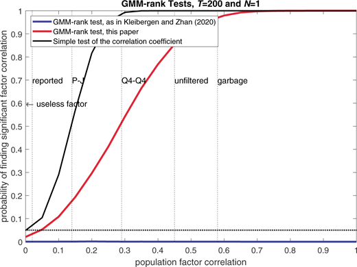
The Power of GMM-Rank Tests:T = 200.
The Power of GMM-Rank Tests:T = 200.
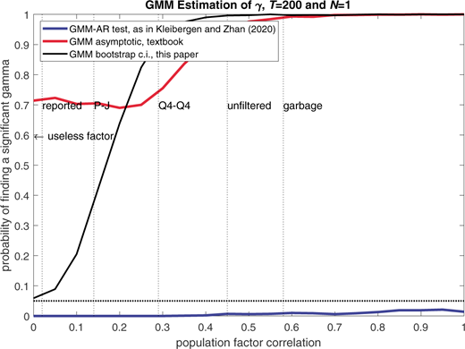
The Power of GMM-Based Inference on the Coefficient of Relative Risk Aversion: T = 200.
The Power of GMM-Based Inference on the Coefficient of Relative Risk Aversion: T = 200.
Analysis of Alternative Power Curves for the Fama-MacBeth Method
Kleibergen and Zhan (2020) provide power curves to “briefly illustrate the malfunction” (p. 524) of the Fama-MacBeth method (their Figures 3 and 4). These power curves show the probability to reject the true hypothesis λ= 2 at various hypothetical values. A test with a correct size should reject with a probability of 5% at λ= 2 and ideally 100% of the time at all other values. Whenever testing the power of a test, however, the assumed alternative matters. Kleibergen and Zhan (2020) assume the following data generating process:
where is the de-meaned risk factor, et,i is the idiosyncratic risk, and λ varies between −1 and 5 across the alternatives. They then check the probability of the Fama-MacBeth t-test, or the simple GRS-test, to reject λ = 2. Surprisingly, they do not report the GRS-FAR test, even though this is claimed in the caption to the according figure.
In economic terms, this data generating process has the feature that the asset pricing model is assumed to be correctly specified. The pricing errors (in excess of λ0) are always zero at one particular value λ.
It is important to think about in which kind of situations this is a relevant case. First, a researcher has to believe that the consumption-based model is literally true (except for λ0) and is concerned about finding the correct price of risk, . But in this setting, the risk factor will always be equally correlated with the returns for all tested s. Even when λ= 0. For the chosen data generating process, it is easy to verify that Corris independent of λ. For all tested alternative hypotheses, the population correlation with the test assets is identical. In the case of the alternative consumption measures, this correlation is about 40% and more for the market excess return.
Second, by changing λ, we also change the mean returns of the test assets . For negative values of λ, the test asset excess returns (in excess of the common pricing error, λ0) will be negative.44They will be around zero for λ= 0. They will be about 2.5 times as large (!) as in the empirical data for λ= 5. These are hypothetical test assets that are not encountered in applied research. While potentially interesting from an econometric perspective, they are mainly irrelevant scenarios from the view of applied research. The test assets are (to a large extend) given and we want to know how risk factors with different strength compare, and not the other way around.
I replicate their power curve (red/grey dotted) in Figure A.3 for the 31 test assets and unfiltered consumption.45In their according Figure 4 (“Power curves of the GRS-FAR Test”), they only show the power curve of the GRS-test, assuming that λ= 2 is known to the researcher.46 I complement these earlier results by adding the actual GRS-FAR test to the picture (red/grey solid). Even more importantly, Kleibergen and Zhan (2020) do only show results when the factor explains the mean returns perfectly (left sub-figure). But this case is empirically irrelevant. Therefore, I add a sub-figure to the right that imposes the empirical pricing errors in the population. In this scenario, I find that the GRS-FAR test will usually not reject the null λ= 2, the power curve is mainly flat.
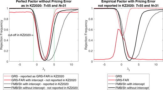
FMB-Shanken and GRS-FAR Power Curves with Varying the Test Assets (Lambda): T = 55.
FMB-Shanken and GRS-FAR Power Curves with Varying the Test Assets (Lambda): T = 55.
One can observe a hump in the power curve around λ= 0. The reason is that the data generating process changes the mean returns of the test assets. Around λ= 0, there is not much mean return left to explain, and as a result the alphas in the GRS-test are tiny and often insignificant. But such test assets do not exist in applied research; or they are avoided, as there would be literally nothing to explain in the first place. Put differently, this data generating process does not capture a situation that can be expected to be found in applied research.
Turning to the Fama-MacBeth/Shanken t-statistics, the black dotted line shows rejection frequencies of the H0: λ= 2 when estimation is with an intercept.
These are the results that are reported by Kleibergen and Zhan (2020). The solid black line shows the according rejection frequencies when estimation is without the intercept; these results are not reported by Kleibergen and Zhan (2020). I also notice that Kleibergen and Zhan (2020) restrict in their figures the displayed area of λ to the range −1 to +5. The restriction on the displayed parameter space changes the interpretation of the figure. While the figure shown in Kleibergen and Zhan (2020) indicates a flat power curve, the power curve is actually sharply increasing just outside the reported area on the right. In addition, when the intercept is not estimated, the power curve is even similar to the GRS-FAR test. When the model is misspecified (right sub-figure), the FMB/Shanken t-statistics remain useful for statistical inference while the GRS-FAR test is clearly not useful for inference on . To the best of my judgment, I am not able to see an obvious “malfunction” of the Fama-MacBeth/Shanken approach in this setting.
Fama-MacBeth Estimation without Intercept
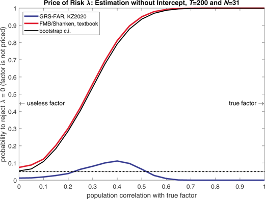
FMB-Shanken and GRS-FAR Power Curves With Varying the Risk Factor (Betas): Misspecified Model, T = 200.
FMB-Shanken and GRS-FAR Power Curves With Varying the Risk Factor (Betas): Misspecified Model, T = 200.
Fama-MacBeth Estimation with Intercept
Additional Simulation Results
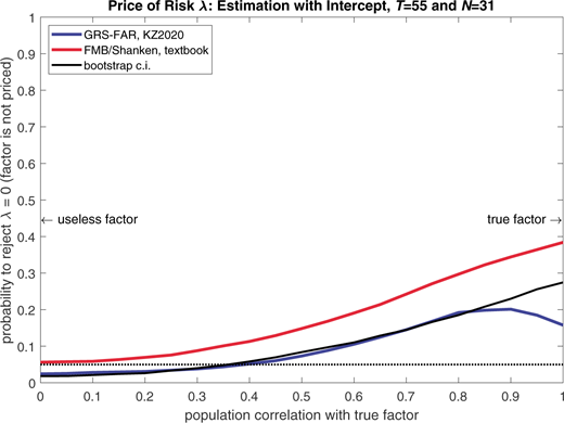
FMB-Shanken and GRS-FAR Power Curves With Varying the Risk Factor (Betas): Misspecified Model, Estimation with Intercept, T = 55.
FMB-Shanken and GRS-FAR Power Curves With Varying the Risk Factor (Betas): Misspecified Model, Estimation with Intercept, T = 55.
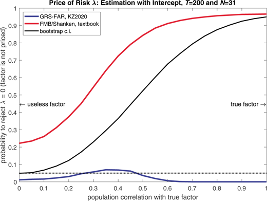
FMB-Shanken and GRS-FAR Power Curves With Varying the Risk Factor (Betas): Misspecified Model, Estimation with Intercept, T = 200.
FMB-Shanken and GRS-FAR Power Curves With Varying the Risk Factor (Betas): Misspecified Model, Estimation with Intercept, T = 200.
Additional Empirical Results
Price of Risk Estimates: Estimation with Intercept.
| Short Sample (1960−2014) | Full Sample (1928−2014) | ||||||
|---|---|---|---|---|---|---|---|
| T = 55 and N = 31 | T =87 and N = 21 | ||||||
| Reported Dec. | Garbage Dec. | P-J Dec. | Q4-Q4 Dec. | Unfiltered T.A. | Reported Dec. | Unfiltered T.A. | |
| const | 7.40 | 1.24 | 4.57 | 0.94 | 1.27 | 9.56 | -0.30 |
| t(const)sh | 3.14 | 0.28 | 1.19 | 0.21 | 0.36 | 3.72 | -0.08 |
| Btrp c.i.95% | (-0.1,11.8) | (-6.5,13.0) | (-2.2,11.7) | (-4.7,11.5) | (-3.4,9.1) | (1.0,14.0) | (-7.0, 6.3) |
| λ | 0.37 | 1.71 | 4.42 | 2.00 | 2.04 | 0.02 | 2.74 |
| t(λ)sh | 0.70 | 1.05 | 1.83 | 1.81 | 1.75 | 0.04 | 2.10 |
| Btrp c.i.95% | (-1.1,1.7) | (-2.1,4.2) | (-1.3,5.2) | (-0.6,2.3) | (-0.4,3.1) | (-2.9,2.6) | (0.7,4.6) |
| GRS-FAR c.i.95% | unbounded | unbounded | unbounded | unbounded | unbounded | (-0.6, 1.2) | (-0.1, 5.0) |
| implied γ | 21.48 | 20.69 | 42.56 | 92.16 | 30.06 | 0.34 | 16.75 |
| t(βALL), p-value | 0.23 | 0.30 | 0.09 | 0.10 | 0.05 | 0.30 | 0.00 |
| F(βi = βj), p-value | 0.26 | 0.47 | 0.49 | 0.53 | 0.37 | 0.00 | 0.00 |
Description: This table complements Table 4 in the main paper and provides results for estimation with an intercept λ0.
Interpretation: When estimation is with an intercept, the Fama-MacBeth/Shanken as well es bootstrap confidence intervals do not indicate a significant price of risk at the 5% level for any of the alternative consumption measures. This result is in line with the lack of power of this specification, as indicated in Figure A.5.
Price of Risk Estimates: Estimation with Intercept, Small Cross-Section.
| Short Sample (1960-2014) | Full Sample (1928-2014) | ||||||
|---|---|---|---|---|---|---|---|
| T = 55 and N = 7 | T = 87 and N = 7 | ||||||
| Reported Dec. | Garbage Dec. | P-J Dec. | Q4-Q4 Dec. | Unfiltered T.A. | Reported Dec. | Unfiltered T.A. | |
| const | 6.98 | 7.29 | 3.24 | −1.33 | −2.73 | 7.10 | −3.50 |
| t(const)sh | 1.87 | 1.67 | 0.72 | −0.23 | −0.61 | 1.60 | −0.73 |
| Btrp c.i.95% | (−6.3,14.7) | (−7.6,23.0) | (−7.9,12.3) | (−15.8,11.0) | (−6.9,11.9) | (−4.1,14.4) | (−11.8,7.7) |
| λ | 1.41 | 0.07 | 4.57 | 2.28 | 3.64 | 2.58 | 4.03 |
| t(λ)sh | 1.57 | 0.05 | 2.10 | 1.92 | 2.18 | 1.63 | 2.21 |
| Btrp c.i.95% | (−1.2,3.6) | (−5.1,4.8) | (0.7,7.9) | (0.1,4.3) | (−2.2,4.8) | (−3.0,4.9) | (0.2,6.2) |
| GRS-FAR c.i.95% | disjointed | disjointed | disjointed | disjointed | (2.3, 5.7) | disjointed | empty |
| implied γ | 80.98 | 0.85 | 44.03 | 104.93 | 53.59 | 53.90 | 24.62 |
| t(βHML), p-value | 0.01 | 0.88 | 0.00 | 0.02 | 0.20 | 0.11 | 0.09 |
| F(βi = βj), p-value | 0.49 | 0.49 | 0.06 | 0.22 | 0.00 | 0.28 | 0.00 |
Description: This table complements Table 5 in the main paper and provides results for estimation with an intercept λ0.
Interpretation: P-J, Q4-Q4, and unfiltered consumption are significandy priced according to bootstrap confidence intervals even in the short sample, when testing with an intercept is likely to become more powerful than with N = 31∕N = 21.
For example, the garbagemeasure (Savov, 2011) comes with a correlation coefficient as large as 0.58, with a bootstrapped 95% confidence interval of h0.3, 0.7i.For unfiltered consumption (Kroencke, 2017) the correlation coefficient is 0.45 h0.2, 0.6i (see Table 1).
The model does not even predict a correlation of 1.00. Individual assets are allowed to have (large) idiosyncratic risk. It is the optimum one can hope for from a purely statistical perspective.
Increasing the sample size to a hypothetical 200 years does not change this conclusion (Appendix, Figure A.1).
See also Cochrane (2005), Chapter 11.5, for a detailed discussion of this frequent problem in the context of asset pricing.
Identification robust inference might be a considerably more critical property in other applications, for example, when there is little theoretical guidance on what magnitude of the parameter to expect.
In addition, the replication code and data used in this paper can be found on the website of the author and the journal.
See, for example, Breeden et al. (1989), Cochrane (2005), Jagannathan and Wang (2007), Burnside (2011).
In empirical work, consumption growth is usually measured as real per capita andreturns are real. In principle, one could also test a nominal version of the model.
Depending on the type of approximation chosen, consumption growth can be measured as simple (e.g., Jagannathan and Wang, 2007) or in logs (e.g., Breeden et al., 1989). The difference between both approximations is usually small in empirical data. I use simple growth rates.
Another way to illustrate the problem of a large is to report the implied risk-free rate, as proposed by Savov (2011),. Because consumption variance is relatively small, large usually implies an unrealistically large risk-free rate, which is also known as the risk-free rate puzzle of Weil (1989). Lengwiler (2004) provides a detailed discussion and a review of the literature.
In principle, small betas might indicate “useless” test assets and not a “useless” factor. The mean excess returns or the dispersion of mean excess returns may be too small for the identification of or . Tests for identification are not tests of asset pricing models.
Among others, Adrian and Shin (2014), Adam et al. (2016), Cujean and Hasler (2017), and Andrei et al. (2019).
Parker and Julliard (2005) proposed a quarterly version of ultimate consumption in their paper. The annual version of ultimate consumption shown in this paper is, therefore, not a fair comparison with the originally proposed measure.
Instead, they report the implied risk-free rate as an indication of how well the model fits the (real) risk-free rate. These estimates are (see Kroencke, 2017), for example, 94%, 30% and 17% for reported consumption, unfiltered consumption and garbage. This shows that the alternative consumption measures can better explain the risk-free rate than reported consumption but still imply too large numbers. The risk-free rate puzzle pointed out by Weil (1989) is mitigated but not resolved. This differs from the statement in Kleibergen and Zhan (2020), Footnote 21.
Kleibergen and Zhan (2020) do not describe the weighting matrix they use for their GMM estimator in the main paper. Instead, they refer to their estimate as “the GMM estimate.” However, one can find the specification of W in their replication code.
This problem is not new in the literature. For example, Cochrane (2005, pp. 215−216) warns about this trap.
For W = 1, the formula for the covariance of gT collapses to S in this special case.
This data generation process is also used in large parts of the analysis by Kleibergen and Zhan (2020).
The direct test is based on the t-statistic: which has N−2 degrees of freedom.
Kleibergen and Zhan (2020, p. 542): “. . . , this rank condition is jeopardized due to the weak correlation between consumption growth and asset returns.”
I use the objective function gTŜ−1 g'T as in Kleibergen and Zhan (2020) to allow for comparisons with their analysis.
Zhan (2010) proposes to utilize the fact that the bootstrap distribution of estimates is quite different between “useless” and “useful” factors to detect a lack of identification. A researcher concerned about weak identification (and not just the over-rejection problem) could conduct such a test or one of the powerful tests reported in Figure 1.
This problem also emerges in the GMM-based tests of the non-linear model, when N > 1.
In the introduction of Kleibergen and Zhan (2020) the following is stated (p. 508): “In this paper, we propose two straightforward asset pricing tests that, unlike traditional tests, are valid for all possible strengths of identification of the risk premia.” One has to digest the paper to find the information that the empirically relevant case of misspecified models does not count as “all possible strengths of identification.”
For a more detailed and complete discussion, see Cochrane (2005), Burnside (2011), and Kleibergen and Zhan (2020).
Shanken (1992) provides the correction term for the standard errors when estimation is with the intercept. When the intercept is imposed to be zero, the correction term for the standard errors can be found in Cochrane (2005), or Burnside (2011), and the replication code to this paper. Kleibergen and Zhan (2020) only include the Shanken correction when they estimate the model with the intercept and omit it when they estimate the model without an intercept.
See, for example, Parker and Julliard (2005).
Kleibergen and Zhan (2020. p. 508): “For instance, Kan and Zhang (1999a) and Kleibergen (2009) warn that the t-test in the FM two-pass procedure can spuriously favor risk factors that are independent of or weakly correlated with asset returns, respectively.”
The results for the estimation with an intercept can be found in the Appendix.
Kroencke (2017) reports a multivariate asymptotic test on the joint significance of consumption betas. Kleibergen and Zhan (2020) show that this test over-rejects and is not reliable.
In additional tests (provided in the replication code to this paper), I find that the multivariate rank test would be powerful for detecting sufficient factor correlation for unfiltered consumption when the data satisfy the normal-i.i.d. assumption. However, I do not provide evidence on the power when the normal-i.i.d. assumption is relaxed.
Alternatively, one could also use the value-weighted market factor, as in Table 1, of course. In fact, Kan and Zhang (1999, p. 228) report that the labor income factor of Jagannathan and Wang (1996) is significantly correlated with the market factor. They state that it is for that reason inappropriate to conclude that labor income is a “useless” factor. However, the “ALL” portfolio better reflects that the Fama-MacBeth regression (or the GRS-FAR test) equally weights the test assets.
For example, for size, book-to-market ratio, and investment decile portfolios, the HML portfolio is long in the five small portfolios, the five high book-to-market ratio portfolios, and the five low total assets growth portfolios and short in the other 15 portfolios. The market portfolio is not included in any of the HML legs. Sorting by the lagged characteristics is equivalent to the formation of the test asset portfolios and does not require forward looking information. However, it is subject to a publication look-ahead bias (we predict stocks before the predictability was discovered), which also applies to the selection of test assets and the multivariate F-test.
I report tests where the cross-sectional intercept is estimated in the Appendix.
My Fama-MacBeth/Shanken t-statistics differ substantially from Table 3 in Kleibergen and Zhan (2020). They do not correct their “NW t-statistics” for the errors in variables problem. Their t-statistics are indeed inflated, but the reason is a problem unrelated to the “useless” factor problem. This fact can be seen from the function “FM_nointercept.m” in the replication code of their paper.
Kleibergen and Zhan (2020, p. 547): “With such limited information in the data, we cannot conclude whether the consumption growth factor explains part of the variation in the cross-section of expected asset returns, nor can we reject the possibility that consumption growth explains all of the variation.”
I also conduct a multivariate test for the significance of the mean excess returns of the test assets. The results are provided in the replication code and do not allow me to conclude that mean returns differ from zero (p-value = 0.39). An analogous univariate test is passed (p-value = 0.00). The multivariate test is also not powerful enough to detect a significant equity premium when N is close to T in the empirical data.
Instead, they switch to a different dataset when analyzing larger T.
These data come directly from Ken French’s website.
The fact that even reported consumption passes the multivariate rank test in the full sample can be attributed to a few test assets. All except one individual beta are insignificant. As mentioned before, the multivariate rank test should not be used as a substitute for a more careful analysis of individual betas to avoid the asset pricing test results being influenced by only a few test assets.
Fama and French (1996) use these six portfolios to construct their SMB and HML factors. It is well known that the decile portfolios and the 25 Fama-French portfolios have a strong factor structure. For that reason, explaining a larger or smaller cross-section of these portfolio sorts is a priori not more or less challenging for a model (see Cochrane, 2011; Daniel and Titman, 2012; Lewellen et al., 2010).
Kleibergen and Zhan (2020) report in their Online Appendix C.3 results for six corner portfolios and the market portfolio. By construction, this cross-section heavily weights the 10% of the smallest companies. In addition, they report results (estimation with intercept) which are not in line with their table caption (estimation without intercept). For example, in the case of unfiltered consumption, the correct results are a p-value for the multivariate rank test of 0.00 and a bounded GRS-FAR c.i. of (1.1, 10.8).
As mentioned before, Parker and Julliard (2005) analyze quarterly sampled three-year consumption and not annual sampled data.
Which would violate the consumption-based asset pricing model and the standard assumption of risk-averse investors (Campbell, 2017).
These are ten decile portfolios sorted by size, book-to-market ratio, and investment plus the market portfolio.
See their replication code, replication_sim.m, lines 83-174. The actual GRS-FAR test has an additional layer of uncertainty, as it accounts for the fact that is unknown to the researcher. The GRS-FAR test is likely to come with less power, as it frequently generates unbounded/disjointed confidence sets and is inconclusive.

