

We estimate the interest rate demand sensitivity of capital goods demand, exploiting a unique dataset and identification method.
High-frequency loan data allow identifying the demand curve using Brazilian data. Institutional setting suggests that interest changes were exogenous to credit demand variation. Promotion effects influence estimates significantly and should be considered when designing credit subsidies and countercyclical investment policies.
Our results indicate a capital good demand sensitivity of −0.40 to −0.50 in credit volume given a 1p.p. increase in interest rates or an elasticity of −2.0 to −2.5. The average loan size elasticity is much smaller, about −0.50, suggesting that the extensive margin is much more sensitive to interest rate changes.
This is one of the few papers in the literature to estimate the elasticity of capital goods credit demand and the first one for Brazil.
Introduction
Demand models provide key inputs in public policy, from tax policy to subsidies. For consumption goods and more acutely for durable goods, temporary price reductions (promotions) are a frequently used marketing tool. This should generate biases in the price elasticity of demand estimates as consumers shift their consumption over time to take advantage of the temporary lower prices (stockpiling, see, e.g. Dubé, 2018). Coglieanese, Davis, Kilian, and Stock (2017) provide a simple dynamic model solution to the promotion bias under the assumption of known, exogenous to the relevant market, promotion shifts. We use this method in a case study of capital goods demand loans provided by BNDES, the Brazilian national development bank.
The PSI program we explore created a special, temporary, subsidy in the financial cost to some BNDES loans, including regular FINAME loans, the main BNDES line of credit for capital goods. The interest rate subsidy was coupled by expanded funding to BNDES from the Treasury to foster economic growth [1].
FINAME is a form of directed credit, where BNDES provides the funds to financial intermediaries (commercial banks and other financial institutions, such as credit cooperatives), also known as second tier public credit. These financial intermediaries provide credit screening and contract with the firm interested in purchasing a capital good from a list of BNDES suppliers. In regular FINAME loans BNDES charges a low interest rate (TJLP) plus a financial fee of up to 2.5p.p. a.a. and banks can mark-up on this rate. This mark-up responds to market forces and client risk profiles (banks bear the default risk). This margin is generally from 2 to 5p.p. (see, e.g. Grimaldi, Machado, & Albuquerque, 2014). The final rate to the firm could vary significantly from firm to firm and bank to bank. PSI loans interest rates were set by the government as fixed nominal rates and included the bank margins (fixed at 3p.p. or 1.7p.p. depending on the firm size). Credit takers knew in advance the financial costs over the course of the loan repayment.
PSI provides an opportunity to learn about the effect of interest rates on credit demand for capital goods investment. The interest rate was set by the government and not determined endogenously due to supply and demand shocks, providing an opportunity to identify the credit demand interest rate elasticity. The available funds for loans were determined by the government also, to meet the expected increases in investment, effectively providing a perfectly elastic supply curve. The Treasury provided ample funding for BNDES over that period and there was no information of credit shortage or rationing, even under the subsidized rates.
This government set credit rate imply that changes in the supply curve were not due to (possibly unobserved) funding decisions by banks, with adjusted market rates, nor did the rate adjusted for short term unobserved credit demand fluctuation. The federal government varied the PSI rate based on an aggregate, economy wide economic growth target, using PSI as an active macroeconomic tool, with ample funding by the Treasury to the credit amounts or the interest rate subsidy. Last but not least, there are a good number of interest rate changes to create time variation in interest rates for identification over time (9 program changes in 65 months).
Estimates of interest rate sensitivity of capital goods demand are rate in the literature. There is a large body of (older) literature on the interest rate elasticity of investment (total firm investment), traced up to Guiso, Kashyap, Panetta, and Terlizzese (2002). Investment demand equations from factor adjustment cost hypothesis would lead to an investment over capital stock demand equation. Investment equations are also studied with more complex adjustment dynamics as surveyed in Bond and VanReenen (2007), from a firm perspective. We have very detailed loan transactions, but no firm information, used in the credit demand literature.
Estimates of credit demand for the goods treated here are hard to find. Most of the recent literature on interest rates and investment by firms focus on reduced form natural experiments to measure the impact of the credit subsidy on outcome variables, as Criscuolo, Martin, Overman, and Van Reenen (2019). Karlan and Zinman (2019) find very large elasticity estimates (from −1.1. to −2.9) of credit interest rate elasticity, from a field experiment on microcredit lending dealing with 20p.p. reductions in level 100APR loans. Our APR rates are much lower, from 3 to 10APR (or 10%a.a.). General effects of BNDES credit, usually in the form of differences-in-differences regressions, are surveyed in Barboza, Pessoa, Roitman, and Ribeiro (2023).
A challenge to estimating the interest rate sensitivity is that the program was repeatedly announced to end, only to be expanded. This produced an anticipation effect in contracted credit, much similar to retail sales or promotions. Given the notice that the interest discounts available through PSI would be over (and given that the purchased capital good can be stocked), firms would anticipate their capital expenditures. Promotions and consumption anticipation would generate an upward bias in the absolute value of demand elasticity, as the period before an expected program end (before an increase in interest rates on loans) would see a rush towards purchases of capital goods and a sharp decrease in credit outlays after the interest rate increase.
Coglianese et al. (2017) explore the same anticipation bias in their demand for gasoline estimates. The proposed solution to the anticipation bias of purchases is simple, namely including lead price variables in the demand estimation. Lead values could be used as gasoline price hikes due to tax increases (used as instrumental variable to act as supply shifts to identify demand) would be known in advance, due to a lag between the legislative passing of the tax change and the inception of the change. We do not use instrumental variables here as the interest rates were determined exogenously by the government and we do not face a similar identification problem. In our case, the next month (lead) price is part of the investing firm information set at period t as BNDES would determine in advance the time frame for the special PSI conditions of the FINAME loans.
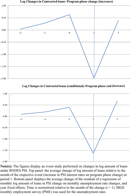
The anticipation effects are very large. An event study for a program phase end as the event, we estimate an average 0.60 log increase in contracted loans in the month before an interest rate hike, a −2.0 log decrease in the month after the program phase end, partially compensated by a 0.45 log increase in the second month after the program change.
Moving to the results, our estimates suggest that in the long run a 1p.p. increase in interest rate would lead to an expected decrease of −0.50 in log credit outlays for machinery and equipment and a −0.45 decrease in log credit outlays for trucks and buses. The effect of an interest rate increase is smaller for the average loan size (−0.10/-0.04, respectively), indicating that most of the sensitivity of credit to interest rate is on the extensive margin (more firms contracting). At mean interest rates these effects can be read as volume credit demand elasticity of −2.50 for machinery and equipment (−2.25 for trucks and buses) and smaller, inelastic −0.5 (−0.2) interest rate elasticity for average size loans.
The note is organized as follows. The next section presents descriptive statistics on PSI and the main program credit lines. The following section presents a preliminary event study that highlights the anticipatory behavior by firms in the face of expected PSI program end (or interest rate increases). The anticipation seems economically significant. The third section presents the credit demand elasticity estimates and the last section collects concluding comments.
The evolution of PSI operations for domestic capital goods
Data collected at BNDES provided information on each FINAME loan from 2002–2015, covering the PSI period September/2009-December/2015. The data on the more than a million loans tells us about whether it was a regular FINAME loan or under PSI conditions, the credit amount and the total financial cost of the loan [2].
We develop our analysis at the PSI sub-program level (for example, capital goods in general; buses and trucks). We compile information on rates and volumes of credit operations by sub-program and month, to estimate a credit interest rate demand semi-elasticity.
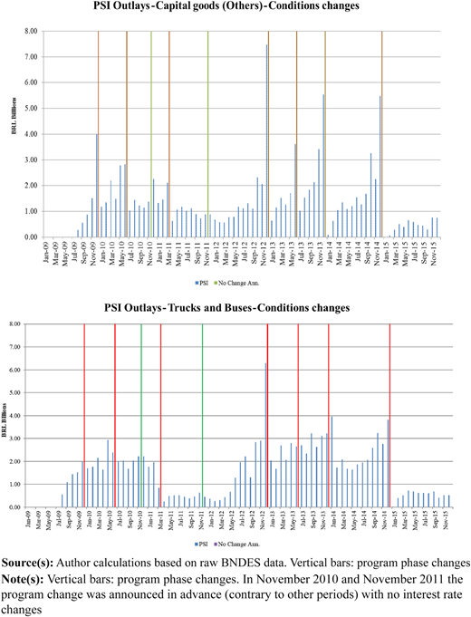
Figure 1 presents the monthly credit contracted totals from 2009–2015 on FINAME and FINAME-PSI loans. We highlight the dates with financial conditions changes, the so called “phases” of PSI. Information on these phases on loan terms and conditions were collected from BNDES public documents (“circulares”) [3]. In general the program/phase was announced well in advance (usually at the phase start) to end at month M. Only a few days before the phase deadline or, often, after month M the program extension and new conditions were announced. There are about nine major phases. See Frischtak, Pazarbasioglu-Dutz, Byskov, and Perez (2017) and WorldBank (2016) for a detailed description of the program. In every phase but for the start of the program in 2009 and in the March 2012 and September 2012 changes, interest rates rose with respect to the previous phase.
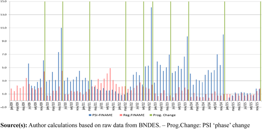
Monthly contracted loan totals under PSI/FINAME and regular FINAME and PSI phases – BRL billions
Monthly contracted loan totals under PSI/FINAME and regular FINAME and PSI phases – BRL billions
A first glance of Figure 1 highlights the anticipatory effect at program phase closing. For example, from August to November 2009, outlays hovered around BRL 2.5 billion a month. In December 2009, when the program was first expected to finish (or face conditions changes) loan contracting more than doubled, reaching BRL 6 billion. The highest level of contracting was in the last month of the lowest rate conditions (Dec. 2012). Interest rates were set to 2.5% in September 2012 and were simultaneously announced to increase to 7% by January 2013. The lack of anticipatory behavior associated with program phase end in March 2012 and November 2012 can be explained by announcements of program expansions in advance, i.e. before the phase deadline (February 2011 and 2012, respectively), contrary to other phases.
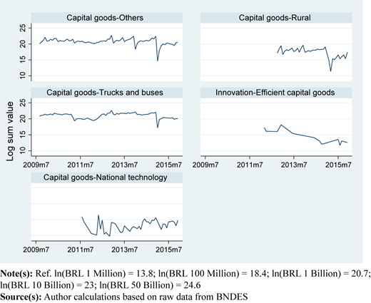
Breaking up the outlays by subprograms (Figure 2), we see that there is considerable heterogeneity in credit demand levels and dynamics across PSI/FINAME sub programs. The two main subprograms on indirect operations, that accounted for more than 95% of total outlays in PSI were trucks and buses and capital goods in general(other).
Interest rates varied significantly over the period, from the low of 2.5% (0.025) to a maximum of 10% (0.1), and across programs (Figure 3). Often the rates were differentiated between large firms and micro, small and medium firms (MSME). Short time variation within phases is due to the composition effect of loans. The mean rate is loan amount weighted.
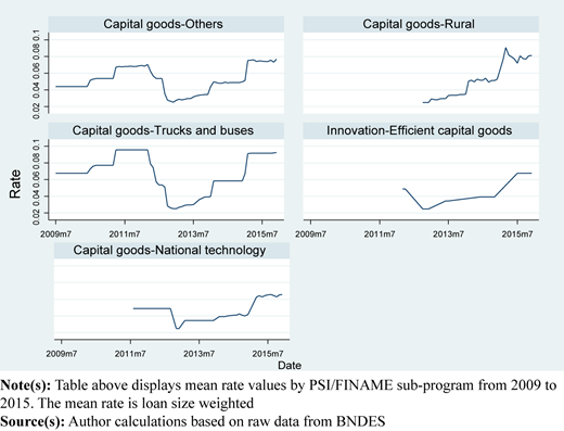
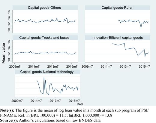
Figure 4 explores the mean loan value. The time evolution is much more stable than the total amount, suggesting that a significant part of the variation in subprogram outlays (Figure 2 above) is the number of loans, not the amount of a loan itself. The visible differences in the aggregate data between mean loan values and total loan values, by subprogram, raise the possibility of finding different effects of interest rates on the intensive and extensive margins, respectively.
Log mean value of capital goods – others and capital goods trucks and buses PSI sub-programs by month (2009–2015)
Log mean value of capital goods – others and capital goods trucks and buses PSI sub-programs by month (2009–2015)
Focusing on the main PSI sub-programs, “Capital goods – Other” and “Capital goods – Trucks and buses” we describe the anticipatory effects in Figure 5. Not surprisingly, the very month before a program phase end there is a surge in credit outlays, as seen in the aggregate data (Figure 1). “Capital goods – Trucks and Buses” display a relatively smaller variation. Note that interest rates for the latter were higher (smaller subsidy with respect to regular FINAME loans) and changed less often. We guide our further analysis on these two sub-programs.
Total monthly outlays for capital goods – others and capital goods trucks and buses PSI/FINAME sub-program (2009–2015) in BRL billions
Total monthly outlays for capital goods – others and capital goods trucks and buses PSI/FINAME sub-program (2009–2015) in BRL billions
Evidence on anticipation effects
The price elasticity of demand can be seriously biased due to an anticipatory behavior from agents as in Coglianese et al. (2017). The authors observe that before a gasoline tax hike came into effect, agents tended to anticipate their consumption. This would lead to biased OLS estimation of a price elasticity of gasoline demand. Coglianese et al. (2017) perform an event study to demonstrate the existence of this phenomena using gas tax changes as the events and observing how the gas consumption systematically increased in the period previous to the price change, only to fall significantly at the price increase period and to rebound in the period after the increase. We conduct a similar event study using as event announced increases in PSI interest rates (either as pre-announced interest increase in a new phase or the end of a phase with no announced extension of the program) and observing credit volume response in nearby periods.
We develop this event study in two ways. First, we observe how the growth of monthly log loan values in a period respond to increases in PSI interest rates. Time is normalized relative to the month of the change. The growth of log total contracted value at the eight recorded events of potential anticipatory behavior are averaged and presented in the top panel of Figure 6 below. In the bottom panel of Figure 6, similarly to Coglianese et al. (2017), we present the same averaged log loans changes conditional on market conditions. The conditional analysis is based on residuals of a regression of changes log values of PSI loans, by month, on the changes in unemployment rate and year fixed effects.
Event study of changes in PSI/FINAME program phases and interest rates growth on BNDES PSI loan amounts
Event study of changes in PSI/FINAME program phases and interest rates growth on BNDES PSI loan amounts
The anticipation seems concentrated on the month before the change, with a more than 0.50 log change (more than 50% increase) in contracted loan average size. The anticipation builds up from a 20% increase in the two months before the change. In a month when the new higher rate is in effect, loans fall by 85% (−2 in log change) on average. This dip is relatively transitory as the next month after the interest rate growth come into effect has an average 50% increase (0.4 in log change). The sum of the effect of the interest change across periods 0, 1 and 2 (the month before, the month of the change and the month following the change, respectively) is −0.94 in log change, half that observed at month 1, where the interest change came into effect. The difference between the observed fall in credit demand at period 1 is even larger in the conditional case, as the observed fall in period 1 of −1.63 in log change is reduced to −0.56 accounting for the anticipation at period 0 and the rebound in period 2.
The anticipation effect provided a misleading effect of the program on aggregate investment rates. As most program phase ends were in December, the fourth quarter aggregate investment rate were inflated with respect to the first quarter, as a large part of the monthly investment rates were anticipated from the first quarter to the last quarter of the previous year, only to generate a large dip in investment levels in the first quarter.
The above figures confirm the relevance of anticipation effects in the demand for credit in the case of PSI/FINAME. Following Coglianesi et al. (2017) we include in the demand estimation lags and also lead interest rates. The results are presented in the next section.
Interest rate sensitivity of capital goods investment
We run an investment demand equation to estimate the interest rate sensitivity. We use data at program level, although we have contract by contract information. As there is no variation in interest rates across contracts within a sub program (but for a few periods with interest rate differences by firm size – large/small firms) running contract or firm level regressions would artificially inflate significance tests in the well-known Moulton effect (Moulton, 1990). We also lack firm level information to estimate a firm level investment demand equation as in Bond, Elston, Mairesse, and Mulkay (2003). For our interest, we explore the high frequency contract data, using monthly data. This provides detailed match between credit amount and loan cost. In the extensive survey of Bond and VanReenen (2007) investment demand functions at the firm level seem the main thrust of the literature mostly for lack of loan data. Firm level data to measure cash flow and capital stocks, key in these firm level investment demand studies, on the other hand, is generally available only at yearly frequency (as in PIA in Brazil). Using more detailed firm data comes at a cost. Using annual data would require the use of average loan cost within a year, muting the interest rate sensitivity of loans. The nature of PSI/FINAME loans on capital goods (not investment projects) explains the repeated use of credit within a year for many firms in the sample. Nevertheless, profitability levels or expectations may be relevant as demand shifters and they are proxied by the unemployment rate and the aggregate Central Bank monetary policy (Inflation Targeting) main rate, the Selic rate. The Selic rate is relevant also to provide a measure of the relative subsidy of the PSI/FINAME loan interest rate. We test whether the model could be restricted to using the PSI loan rate difference over the Selic rate. Regression variables descriptive statistics are presented in the Appendix Table A1.
We choose a log-linear specification with log monthly values of contracted credit at PSI/FINAME in a specific subprogram explained by the financial cost of the loan (interest rate charged) and demand shifters such as the unemployment rate and the economy reference rate (Selic). The estimated coefficient on the loan interest rate is not an elasticity per se, as it measures the effect of a 1p.p. (p.a.) increase in loan cost on log (average) volumes. To explore the differences between the intensive and extensive margin effects we use total loan value and average loan value [4].
Namely, Table 1 presents estimates of regression specifications as
where yit is the dependent variable (log loan volume or log average loan in program i at time t), rit the interest rate of loans in the month, from program i in time t, with lag and lead, dt a dummy for end of phase month, ut the unemployment rate, it the base interest rate -Selic- and x a vector of yearly dummies. Long run effects of interest rates can be calculated with β0 + β−1 + β1.
Interest rate sensitivity on PSI/FINAME loans
| (1) | (2) | (3) | (4) | (5) | (6) | (7) | (8) | (9) | (10) | (11) | (12) | |
|---|---|---|---|---|---|---|---|---|---|---|---|---|
| Variables | Average loan vales | Sum of loan values | ||||||||||
| Samples | Pooled | General capital goods | Capital goods – trucks and buses | Pooled | General capital goods | Capital goods – trucks and buses | ||||||
| Rate | −0.233*** | −0.255*** | −0.310*** | −0.576*** | −0.0740*** | −0.0879*** | −0.145*** | −0.115 | −0.404** | −0.00143 | −0.414*** | −0.143 |
| (0.0217) | (0.0739) | (0.0550) | (0.0844) | (0.0207) | (0.0287) | (0.0535) | (0.162) | (0.177) | (0.273) | (0.0723) | (0.127) | |
| Lag rate | −0.0225 | 0.139** | −0.0190 | 0.357*** | 0.395* | 0.132 | ||||||
| (0.0532) | (0.0644) | (0.0226) | (0.117) | (0.208) | (0.0962) | |||||||
| Lead rate | 0.0600 | 0.334*** | 0.0630* | −0.368*** | −0.906*** | −0.436*** | ||||||
| (0.0548) | (0.0712) | (0.0334) | (0.120) | (0.230) | (0.101) | |||||||
| Dummy end of phase | 0.193* | 0.514*** | 0.133** | 1.070*** | 0.948*** | 0.620*** | ||||||
| (0.102) | (0.104) | (0.0569) | (0.224) | (0.338) | (0.204) | |||||||
| Unemployment rate | 0.00216 | 0.0402 | −0.0580 | 0.0308 | 0.0299 | 0.0547** | 0.126 | 0.142 | 0.264 | 0.194 | 0.105 | 0.0788 |
| (0.0473) | (0.0504) | (0.0574) | (0.0495) | (0.0321) | (0.0269) | (0.117) | (0.111) | (0.185) | (0.160) | (0.109) | (0.0971) | |
| Avg Selic rate | 0.207*** | 0.190*** | 0.210*** | 0.0570 | 0.0836** | 0.0489* | 0.155* | 0.101 | 0.501*** | 0.541*** | 0.294*** | 0.290*** |
| (0.0367) | (0.0374) | (0.0543) | (0.0511) | (0.0315) | (0.0261) | (0.0905) | (0.0821) | (0.175) | (0.165) | (0.107) | (0.100) | |
| Sum of coefficients: Rate + Lag rate + Lead rate | −0.23*** | −0.22*** | −0.31*** | −0.10* | −0.07*** | −0.04** | −0.15*** | −0.13** | −0.40** | −0.51*** | −0.41*** | −0.45*** |
| Rate and Selic coeff. Symmetry test (p-value) | 0.48 | 0.38 | 0.015 | 0.18 | 0.59 | 0.71 | 0.89 | 0.71 | 0.45 | 0.8 | 0.09 | 0.01 |
| AR test (p-value) | 0.00 | 0.00 | 0.18 | 0.64 | 0.00 | 0.013 | 0.00 | 0.00 | 0.67 | 0.98 | 0.764 | 0.95 |
| Observations | 152 | 148 | 76 | 74 | 76 | 74 | 152 | 148 | 76 | 74 | 76 | 74 |
| R-squared | 0.476 | 0.495 | 0.416 | 0.649 | 0.723 | 0.816 | 0.424 | 0.569 | 0.429 | 0.657 | 0.723 | 0.816 |
Note(s): Monthly data by the two main PSI/FINAME subprograms, General Capital Goods (Capital goods – others) and Capital goods – Trucks and Buses from September 2009 to December 2015. Dependent variable: ln(mean contract loan value) for columns 1–6 and ln(total loan contracted) for columns 7–12. Rate is the financial cost of the loan (in annual p.p.). Dummy end of phase is a dummy for a program phase with no pre-announced extension. Unemployment rate is from IBGE in % of the labor force and the Avg Selic rate is the monthly average of the daily reference Selic rate of public debt, used as benchmark rate in the Brazilian economy and monetary levy in the Inflation Targeting inflation policy by the Central Bank. AR test(p-value) is a first order autocorrelation Breush-Godfrey test. Autocorrelation robust standard errors are used when needed in non-pooled cases (column 3). Coefficient significant tests p-value: ***p < 0.01, **p < 0.05, *p < 0.1
Source(s): Author’s calculations based on raw data from BNDES
Results are presented in Table 1. Column 1 presents the pooled data across the two subprograms, Capital Goods in general (“other” in the original description) and Buses and Trucks and other (non-electric) transportation equipment. We see that the mean loan is sensitive to interest rates with the expected negative sign. The demand shifters seem significant, but autocorrelation tests suggest a need for standard error correction. Column 2 expands the simple model in column 1 including a one period (month) lead and lag rate, following Coglianese et al. (2017). The inclusion of these variables does not change the short run or long run (the sum of all rate coefficients) sensitivity.
In all specifications the reference interest rate Selic has the expected positive sign: a 1p.p. increase in the reference rate would make a subsidized loan cheaper, relatively, increasing loans by 0.20 to 0.50. A coefficient restriction hypothesis test does not reject the symmetry between the loan rate and Selic for both models. The unemployment rate effect is less robust, often insignificant or with an unexpected negative sign.
Columns 3 and 4 present the results for the General Capital Goods credit line. Interestingly serial correlation is not present according to a standard Breusch-Godfrey serial correlation test. Lag and Lead rate coefficients are significant and we see a short run estimate of −0.576 and a (significantly different from zero) long run estimate of −0.10, indicating that a 1p.p. increase in the cost of loans would decrease the average loan value by log 0.10, or a little less than 10%. This is much smaller than the short run effect of −0.58, as expected. Lead rate appears significant, although the lag rate is not. We explicitly model a program phase end for those cases where it was not announced the next moth rate. On average such program end would entail an average 0.50 increase in log mean loan size.
Columns 5 and 6 bring the results for the Buses and Trucks credit line. The short run interest rate sensitivity of the average loan in the lead-lag estimate is smaller than the other capital goods case (columns 3 and 4 respectively). Long run effects are below 1/10, i.e. a 1p.p. increase in interest rates would lead to an expected decrease of only 4% in the average loan value.
The next set of columns (7–12) repeat the specifications of columns 1–6 but now using total value of loans (in logs) as dependent variable. The coefficient significance pattern is similar, as well as the higher sensitivity of General Capital Goods compared to Buses and Trucks. The interest rate sensitivity of total loans is always larger than that of mean loan value. For General Capital Goods it increases (in absolute value) from −0.10 to −0.50 and for buses and trucks increases from −0.04 to −0.45, statistically significant in all cases. Phase end effects are very large, more than doubling contracted loans for general capital goods and increasing them more than 80% (log change of 0.62) for buses and trucks. Again, the phase end effects difference between mean loan effects and total (sum) loan effects highlight the intensive margin effect of aggregate investment.
Additional evidence on capital good credit interest rate sensitivity is provided in Tables A2 and A3 in the Appendix. Table A2 present specifications that do not include the program phase end adjustment and measure the effects as elasticities. Note that in this case, the explanatory interest rate is ln(1+rate/100), so a 1p.p. increase is approximately a 0,01 change, explaining the 100 factor increase in rate coefficients. The overall results of significant anticipation effects on interest rate changes, the relevance of the intensive margin to explain aggregate movements in investment and the higher sensitivity of general capital goods compared to buses and trucks are maintained. Table A3 re-estimates the same models with variables in differences. While specification tests indicate that serial correlation is not an issue (with stationary variables and residuals), we run the models in first differences as a worst case of lack of long run effects and nonstationarity. Coefficients change little and the main results listed above appear in these models as well.
Concluding comments
This paper used the case of PSI/FINAME, a credit line by BNDES, the Brazilian Development Bank to finance capital goods purchases (including transportation vehicles) to estimate the sensitivity of credit to interest rates. PSI provides an interesting opportunity to estimate this sensitivity as interest rates (and total financial cost) were set by the government, with additional funding to meet the demand, providing a perfectly elastic supply curve, that shifted over time for reasons unrelated to the demand of the credit line. These exogenous shifts provide the identification of the demand function using market data (prices and quantities). The fair number of rate changes of the program generates sufficient variation in rates to estimate coefficients with precision. The rates changes can be attributed to aggregate, economy wide growth targets, including political business cycles (as in the 2012 election).
Estimates of interest rate sensitivity of capital goods are rare in the literature for lack of identification and available data, with the exception of Guiso et al. (2002). They suggest an elasticity of −1, what would be comparable to a −0.2 coefficient in our models (under a benchmark rate of 5%a.a.). Most of the literature focuses on natural experiments on cost of credit changes in an impact evaluation framework, as in Criscuolo et al. (2019) or focus on total firm investment in Euler-equations/accelerator models as in Bond and VanReenen (2007).
The changes in credit cost, while exogenous with respect to demand, create an econometric issue as firms knew in advance an interest rate change and anticipated behavior accordingly. An expected interest rate increase (or a subsidized interest rate program end) would lead to a rush to tap on the better rates, only to meet a lower demand at the interest rate increase, as firms had anticipated the projected investment outlays. Coglianese et al. (2017) provide a simple solution to this problem, by the inclusion of lead and lag rates in the demand equation.
We document very large anticipation effects descriptively and in an event study framework. The month before a program end or interest rate increase lead to a 50% increase in contracting, with an average 85% decrease in the month of the interest change. In the following month to that of an increase in rates contracting increased by 40% on average.
Including these lead and lag and an indicator for expected program end our econometric estimates point to a long run interest rate sensitivity of circa −0.40/−0.50, with the upper value for General Capital Goods and the lower figure for the Buses and Trucks credit line for total loans contracted. We also estimate the effect on the average loan amount in a contract and the sensitivity is much smaller at −0.10/−0.04 respectively. This points to the relevance of the extensive margin to explain aggregate investment credit demand. The aggregate credit level is more sensitive to the number of firms taking a loan when facing an interest rate decrease than to firms contracting larger loans.
Long run loan interest rate sensitivity seems symmetric to base interest rate (Selic in the Brazilian acronym), suggesting that firms care about the subsidy level (difference between loan rate and the Selic rate) to contract. The PSI/FINAME program was based on strong subsidies to interest rates, over the regular BNDES loan rates. The program hinged on credit to be sensitive to interest rates, so to respond to the cost of capital decrease. It seemed successful in increasing contract levels as interest rates matter. Nevertheless, this interest sensitivity possibly came at the expense of a significant budget cost to the Brazilian Treasury, faced with covering the interest differential and the expanded funding to the loans. At the same time, the expansion in PSI/FINAME contracting could have come with a reduction in regular FINAME contracting. Evaluating whether the PSI/FINAME credit contracting due to the program lower rates only shifted investment from regular FINAME loans and from firms that would invest anyway using other funding (including own) are important questions for further analysis, with early evidence in Grimaldi et al. (2014).
Notes
Operational information on BNDES, including PSI and FINAME can be found in Frischtak et al. (2017).
The underlying microdata was obtained under a special request under the Lei de Acesso a Informação and cannot be shared. Since the original data request, BNDES has posted the loan information at the Central de Downloads part of the BNDES website, under operações indiretas. The data used at the regressions and graphs is available upon request.
The list of “circulares” was provided by BNDES staff. We collected the full text of each “circular” to characterize the phases and conditions on PSI. We acknowledge their support, but claim sole responsibility for the interpretation of the documents.
Denoting total loans at period t as Yt, average loan is given by Yt/n. Using logs is easy to see that ln(average value) = ln(total value) – ln(number of loans). Given that the right hand side has the same variables and values in both specifications, the effect on the number of loans can be measured by differences in the coefficient of ln(total value) and ln(average value).
This paper received funding from the WorldBank as part of a larger Project on Public Expenditures Brazil. Comments from Ceyla Pazarbasioglu, Antonio Nucifora and XXX SBE meetings participants are acknowledged. BNDES loan information was made available by a request for information (SIC). A previous version of the paper was presented at the 2019 CRESSE Conference. A similar data set is available at BNDES website (“operações indiretas” at “Central de Downloads”). BNDES staff provided guidance on the PSI phases on official documents. The interpretation of the results and information provided is my own and should not be associated with BNDES, the WorldBank group or UFRJ. Angelo Marcantonio Júnior provided superb research assistance.
References
The supplementary material for this article can be found online.
