


This paper evaluates the effectiveness of price incentives in reducing residential water demand during the 2014 water shortage.
We utilized a fixed effects panel data model and a diff-in-diff analysis.
The results revealed a significant decrease in water consumption during the early months of the water crisis in all municipalities, with a more pronounced effect in the MRSP compared to cities where price incentives were not applied. We estimate that the price incentives program reduced monthly water consumption by approximately 0.5 m3 per household. We also provide evidence that the impact of the water pressure reduction in pipelines was similar, while the financial burden program appears to have had a weaker effect. Finally, after all the adopted policies had ceased, the water consumption remained lower than the pre-crisis level in all municipalities.
Compared to the existing literature, we used a different control group, based on water consumption in municipalities outside the MRSP and achieved opposing results.
1. Introduction
From 2014 to 2016, the Metropolitan Region of São Paulo (MRSP), Brazil, experienced a “Water Crisis,” a severe water shortage. As a result, the region’s water reservoirs were severely depleted, forcing the semi-public São Paulo State Basic Sanitation Company (SABESP), which manages the reservoirs and operates the water and sewage system in almost all municipalities in the MRSP, to draw water from below the floodgates from the main reservoir, the Cantareira system, for the first time in history. The Cantareira system supplies water for nearly eight million people, 40% of the total population of the MRSP.
During the Water Crisis, the São Paulo State Water and Energy Services Regulatory Agency (ARSESP) authorized SABESP to establish economic incentives – a financial “bonus and burden” program – for reducing water consumption in the MRSP. The financial bonus was implemented in March 2014, and it consisted of a 10% cut in water and sewage tariffs to users who reduced from 10 to 15% of the monthly average water consumption. Those users who reduced consumption from 15 to 20% got a 20% tariff cut, and those who reduced by 20 or more got a 30% tariff cut. The baseline was the monthly average water consumption from February 2013 to January 2014 (ARSESP, 2014a, b, c; see Figure 1). These economic incentives covered over 17 m people and 31 municipalities in the state of São Paulo, mainly in the MRSP. The program started in February 2014 and was withdrawn in March 2016.
 The vertical bar chart is divided by a vertical dashed line into two sections titled “Bonus Tariff cut (negative) March 2014” on the left and “Burden Tariff increase (positive) January 2015” on the right, with the horizontal axis labeled “Water Consumption variation (monthly)” and category labels from left to right “less than negative 20 percent”, “From negative 15 percent to negative 20 percent”, “From negative 10 percent to negative 15 percent”, “From negative 10 percent to 0”, “From 0 to positive 20 percent”, and “greater than positive 20 percent”. The data for the bars are shown as follows: “Water Consumption variation (monthly)”: less than negative 20 percent, “Bonus Tariff cut (negative) March 2014”: negative 30 percent. “Water Consumption variation (monthly)”: From negative 15 percent to negative 20 percent, “Bonus Tariff cut (negative) March 2014”: negative 20 percent. “Water Consumption variation (monthly)”: From negative 10 percent to negative 15 percent, “Bonus Tariff cut (negative) March 2014”: negative 10 percent. “Water Consumption variation (monthly)”: From negative 10 percent to 0, a dashed vertical line is shown. “Water Consumption variation (monthly)”: From 0 to positive 20 percent, “Burden Tariff increase (positive) January 2015”: 40 percent. “Water Consumption variation (monthly)”: greater than positive 20 percent, “Burden Tariff increase (positive) January 2015”: 100 percent.
SABESP financial bonus and burden program. Baseline: average consumption for each household between February 2013 and January 2014. Source: SABESP (https://site.sabesp.com.br/site/interna/Default.aspx?secaoId=551 and ARSESP (2014a, b)
The vertical bar chart is divided by a vertical dashed line into two sections titled “Bonus Tariff cut (negative) March 2014” on the left and “Burden Tariff increase (positive) January 2015” on the right, with the horizontal axis labeled “Water Consumption variation (monthly)” and category labels from left to right “less than negative 20 percent”, “From negative 15 percent to negative 20 percent”, “From negative 10 percent to negative 15 percent”, “From negative 10 percent to 0”, “From 0 to positive 20 percent”, and “greater than positive 20 percent”. The data for the bars are shown as follows: “Water Consumption variation (monthly)”: less than negative 20 percent, “Bonus Tariff cut (negative) March 2014”: negative 30 percent. “Water Consumption variation (monthly)”: From negative 15 percent to negative 20 percent, “Bonus Tariff cut (negative) March 2014”: negative 20 percent. “Water Consumption variation (monthly)”: From negative 10 percent to negative 15 percent, “Bonus Tariff cut (negative) March 2014”: negative 10 percent. “Water Consumption variation (monthly)”: From negative 10 percent to 0, a dashed vertical line is shown. “Water Consumption variation (monthly)”: From 0 to positive 20 percent, “Burden Tariff increase (positive) January 2015”: 40 percent. “Water Consumption variation (monthly)”: greater than positive 20 percent, “Burden Tariff increase (positive) January 2015”: 100 percent.SABESP financial bonus and burden program. Baseline: average consumption for each household between February 2013 and January 2014. Source: SABESP (https://site.sabesp.com.br/site/interna/Default.aspx?secaoId=551 and ARSESP (2014a, b)
At the same time, the São Paulo State government launched a state-wide public campaign to make the population aware of the importance of saving water, targeting all municipalities in the state of São Paulo, not only those affected by the Water Crisis.
With the Water Crisis worsening at the end of 2014, SABESP officials announced in November 2014 a long-term water pressure reduction in the MRSP pipes [1]. Furthermore, in January 2015, SABESP also implemented a financial burden program consisting of a 40% increase over the tariff applicable to water consumption that exceeds up to 20% of the monthly average and a 100% increase for the part that exceeds this threshold.
The combination of these policies may have had both immediate and long-term effects. Households may have immediately reacted to the stimulus provided by the policies, reducing water consumption, and they may also have been encouraged to invest in water tanks and water-saving toilets and to make long-term behavioral changes regarding water consumption (Janmaat, 2018).
We use a diff-in-diff methodology to evaluate the effectiveness of the financial bonus program implemented in March 2014 in reducing residential water demand. It also provides evidence about the impact of other approaches used by SABESP in the MRSP to influence residential water demand, such as the water pressure reduction in the pipelines and the financial burden program. Additionally, we evaluate whether the water consumption level remained lower than the pre-crisis level after the end of the crisis and the end of the water-saving policies adopted.
Souza and Fouto (2019), Souza, Teixeira, and Fouto (2021) and Grover and Lucinda (2020) also studied the economic incentives for reducing water consumption adopted in the MRSP. Still, neither had information about municipalities outside the MRSP, where financial incentives were not implemented. Grover and Lucinda (2020) separated control and treatment groups among a sample of households in the MRSP to measure the effects of the financial bonus and burden program. We used a different control group, based on water consumption in municipalities outside the MRSP and achieved opposing results.
Analyzing the overall impact of water conservation policies tends to be more relevant as water shortage episodes become more frequent following increasing urbanization and the effects of climate change.
2. Water demand and the impact of policies to reduce water consumption.
The effectiveness of price and non-price incentives for water conservation has been the aim of several studies. Renwick and Archibald (1998) analyzed the extent to which price and alternative policy instruments (such as use and quantity restrictions and subsidies for water-efficient technologies) reduce residential demand and their distributional implications by type of household. Their study utilized detailed household-level panel data for two California communities. Their findings suggest that the effectiveness of demand-side management policies in reducing aggregate demand and distributing water savings among household classes depends on the selected policy instrument and aggregate demand composition. Price responsiveness was found to vary by income group, with lower-income households being more price-responsive than relatively wealthy households [2]. These results suggest that, with all other factors held constant, price policy will significantly reduce residential demand in a lower-income community than in a higher-income community.
Corral, Fisher, and Hatch (1999) developed a model of residential water demand to study the influence of pricing and non-price conservation programs on consumption and conservation behavior in three water districts in the San Francisco Bay Area over 10 years, including drought and average years. Price strategies included nonlinear or block pricing; non-price programs included water conservation education, supply restrictions and low-flow plumbing. Contrary to Renwick and Archibald, they utilized aggregated or district-level data. Their findings showed that pricing could effectively reduce water consumption, particularly during the annual dry season and longer drought episodes. The effect is mitigated when non-price conservation programs are included in the analysis. Among these, use restrictions and landscaping audits are particularly effective in inducing conservation.
Olmstead and Stavins (2009) also compared price to non-price approaches to urban water conservation. The non-price (or command and control) policies considered were rationing in the short run and adopting technology standards in the long run. Their analysis emphasizes the emerging theoretical and empirical evidence that using prices to manage water demand is more cost-effective than implementing non-price conservation programs. Price-based approaches may also compare favorably to command-and-control approaches regarding monitoring and enforcement. However, they also emphasize equity and distributional considerations, concluding that neither policy instrument has a natural advantage in terms of equity [3].
Lu, Deller, and Hviid (2018) review the international evidence on increasing block tariffs (IBTs) and behavioral interventions to manage residential water demand. They highlight the challenges of implementing effective IBTs and discuss how behavioral interventions may be adopted as a substitute or complement to price interventions. Furthermore, they assess whether the evidence is still valid in settings beyond drought-prone areas.
Still, regarding non-price incentives, Wang, Chiang, and Liou (2019) studied the effectiveness of a water-saving educational program on consumers’ behavior, assessing the effectiveness and the learning achievements of public participation in water-saving activities in a museum exhibition. For that purpose, museum visitors completed pre-test and post-test questionnaires upon arrival at the exhibition’s end. The questionnaires asked respondents directly about their knowledge of water and habits. Researchers gathered 620 valid questionnaires for those over 18. The results showed a medium-small but significant improvement in the water literacy of the subjects after the water-saving activities. Still, there was no significant correlation between water knowledge and water attitude before or after the activities.
Meyer, Jacobs, Westman, and McKenzie (2018) discuss the effect of pressure adjustments on individual consumer water demand in South Africa. They monitored water pressures and flow rates at a few strategic locations and 44 separate homes during controlled pressure adjustments. Their findings showed a positive relationship between the average pressure change (P) and median consumer demand (Q), where reduced pressure led to reduced demand. The linear model suggested a relationship of ΔQ ≈ 0.5ΔP between the change in average pressure and the change in median consumer demand at a consumer connection. They also noted practical limits to the level of pressure reduction that can be attained, beyond which the consumers become unsatisfied with the pressure.
In Brazil, Souza and Fouto (2019) and Souza, Teixeira, and Fouto (2021) analyzed policies for water consumption reduction during the 2014–2016 Water Crisis in the MRSP. The former details the SABESP “bonus and financial burden” program and analyzes its impact on the monthly average consumption per household in 25 districts of São Paulo. They used a panel data model with data ranging from January 2013 to July 2015, and time variables (month and year) were used as controls. They concluded that the SABESP program could be considered “a valid solution for lowering water demand” since “(1) the implementation was effective in encouraging water consumption reduction and more efficient than the contingency tariff, and (2) consumption reduction was more meaningful in districts that used water originating from springs under more critical conditions but were adopted by citizens from all analyzed districts” (Souza & Fouto, 2019, p. 1277). The econometric analysis also demonstrated that “income was relevant for water demand reduction; ” that is, “districts in higher social classes were more willing to reduce consumption” (Souza & Fouto, 2019, p. 1277). Interestingly, the authors noted a decrease in water consumption in all districts, even those without the financial bonus. They called this movement the “awareness effect,” which influenced the severity of the water crisis in the city (p. 1272).
Two years later, Souza et al. (2021) investigated whether the scarcity period and the SABESP program had a persistent impact on consumer behavior after the water crisis was over. They used a hierarchical linear model with three levels (HLM3) to verify whether the reduction effect remained in the midterm and a panel data regression model to understand which factors influenced water consumption behavior changes before, during and after the local severe water drought. Once again, their study used the monthly average consumption of districts in São Paulo; however, this time, the data ranged from January 2013 to September 2019. The explanatory variables included the average household income and the percentage of women living in each district. According to the authors, the latter variable was included “since the literature points out that women tend to act more environmentally consciously (Meinzen-Dick, Kovarick, & Quisumbing, 2014) and, therefore, may consume water more rationally” (Souza et al., 2021, p. 5). They concluded that the average water consumption level after the rain scarcity period was significantly lower than before and that, in addition to the economic incentives, the severity of the scarcity event explained the behavior change verified in water consumption [4].
Grover and Lucinda (2020) also evaluated the policy response to the 2014–2015 drought in São Paulo. They used very detailed microdata on household water consumption and a difference-in-difference design, which allowed them to infer causality. They concluded that the financial burden instrument induced household conservation behavior, but the bonus did not. The authors then turned to the political budget cycle theory to explain why the reward-based instrument, which was deemed both “ineffective and expensive,” was implemented. Grover and Lucinda (2020) used a sample of 340 households in the city of São Paulo, 157 of them were served by the Cantareira System and were exposed to the bonus program since March 2014, while the others were exposed to the program only two months later. Interestingly, the authors used information on which neighborhoods were fitted with pressure reduction valves (PRVs), trying to filter out the effect of the water pressure reduction, which could confound the impact of the bonus program on water consumption.
However, neither Souza and Fouto (2019), Souza, Teixeira, and Fouto (2021) nor Grover and Lucinda (2020) analyzed the effect of the price incentives on water consumption, controlling for the impact of the state-wide public campaign and using other municipalities outside MRSP as a control group. Our contribution complemented their analysis with a different control group and new results.
3. Methodology
Differing from the approaches taken by Souza and Fouto (2019), Souza, Teixeira, and Fouto (2021) and Grover and Lucinda (2020), our study incorporates water consumption data from all municipalities in the State of São Paulo served by SABESP, rather than solely focusing on districts within the city of São Paulo. This enables us to test the causal relation between the price incentives program implemented exclusively in the MRSP and water consumption while controlling other factors, such as the effects of the educational campaign initiated by the State of São Paulo government targeting all municipalities.
We adopted a diff-in-diff (DiD) methodology using a fixed effects panel data model to measure the effect of the price incentives program (financial bonus program), implemented exclusively in the MRSP, on water consumption. The treatment group consisted of the 38 MRSP municipalities that experienced a severe water crisis. The control group consisted of 324 municipalities served by the same State of São Paulo water operator, which did not participate in the SABESP program. The treatment and the control groups’ municipalities are shown in Figure 2.
 The image shows a map with labeled regions including “Sao Paulo”, “Campinas”, “Ribeirao Preto”, “Rio de Janeiro”, “Juiz de Fora”, “Contagem”, “Londrina”, “Curitiba”, “Parana”, and “Grosso do Sul”, with numerous small markers distributed across the map where green markers represent the control group and red markers represent the treatment group. Green markers are spread widely across areas around Sao Paulo, Campinas, Ribeirao Preto, Londrina, and Curitiba, while red markers are concentrated near the coastal region around Rio de Janeiro and parts of Sao Paulo. A legend appears in the bottom right corner labeled “Control Group” with a green color and “Treatment Group” with a red color.
The treatment group (the Metropolitan Region of São Paulo) and the control group (all other SABESP municipalities). Source: Elaborated by the authors
The image shows a map with labeled regions including “Sao Paulo”, “Campinas”, “Ribeirao Preto”, “Rio de Janeiro”, “Juiz de Fora”, “Contagem”, “Londrina”, “Curitiba”, “Parana”, and “Grosso do Sul”, with numerous small markers distributed across the map where green markers represent the control group and red markers represent the treatment group. Green markers are spread widely across areas around Sao Paulo, Campinas, Ribeirao Preto, Londrina, and Curitiba, while red markers are concentrated near the coastal region around Rio de Janeiro and parts of Sao Paulo. A legend appears in the bottom right corner labeled “Control Group” with a green color and “Treatment Group” with a red color.The treatment group (the Metropolitan Region of São Paulo) and the control group (all other SABESP municipalities). Source: Elaborated by the authors
Water consumption data from SABESP shows the monthly volume of water consumed in each municipality by categories (social-residential, residential, commercial and industrial) and by consumption ranges (blocks). In this study, we used only the “Residential” category since we aim to study the impact of price incentives on residential water demand. The water tariff is considerably lower in the “social-residential” category of households [5].
The price incentives program started in March 2014. A few months later, SABESP also announced additional policies, including a long-term reduction in water pressure in the MRSP’s pipelines in November 2014 and a financial burden program in January 2015. Between March 2014 and October 2014, the price incentives program operated while the water pressure in pipes in the MRSP was marginally reduced compared to the pre-crisis level [6].
The São Paulo State’s Regulatory Agency for Energy and Water Services (ARSESP) authorized the SABESP “bonus and financial burden” program in February 2014. The program started in March 2014 and ended in March 2016. We collected data from January 2012 to December 2018. We used the 25 months of the “bonus and financial burden” program as a proxy for the water crisis period and its end as a proxy for the end of the water pressure reduction in pipes. Table 1 specifies the periods observed before and after the water crisis and the dates when each policy adopted in the MRSP began and ended. The financial bonus program was implemented in March 2014, marking the beginning of the Water Crisis. The water pressure reduction in pipes was announced in November 2014, and the financial burden program was implemented in January 2015. These three policies ended in March 2016, marking the end of the water crisis.
Periods before and after the water crisis and periods in which the policies were active
| Before the water Crisis | First period | Second period | Third period | After the water crisis |
|---|---|---|---|---|
| 26 Months (Jan 2012 - Feb 2014) No water conservation policy was active | 8 Months (Mar 2014 - Oct 2014) Only the financial bonus program is active | 2 Months (Nov 2014 - Dec 2014) Pressure reduction in water pipelines is also active | 15 Months (Jan 2015 - Mar 2016) The financial burden program is also active | 33 Months (Apr, 2016 - Dec 2018) All policies ended in March 2016. No policies active |
Note(s): The statewide public campaign started in the first period and remained active until the end of the third period
Source(s): Elaborated by the authors
The DID is a double difference method. The first difference is between the average dependent variable post- and pre-experiment for the treatment () and the control groups (). The second difference is between the observed differences in the treatment and the control groups () [7]. However, the treatment effect can also be assessed using a fixed-effects model for panel data, which controls all characteristics fixed in time for each municipality, considerably reducing the possibility of omission bias in the estimators.
3.1 Water availability in the MRSP and the “awareness effect”
On February 1st, 2014, the water volume available to the MRSP was 37.9% of the storage capacity in all reservoirs. The largest MRSP reservoir, the Cantareira system, was at 21.9%. Water availability had been declining since mid-2013. On November 1st, 2014, when the water pressure reduction was announced, the available water volume was only 1.9% of the storage capacity and the Cantareira system was almost 20% “negative,” meaning below the floodgate, a desperately severe situation. On March 1st, 2016, when the water crisis ended, the observed level was 38.1% of the storage capacity and the Cantareira system was 24.0% “positive,” back to its regular availability (see Graph 1).
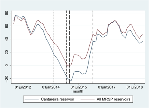
Monthly volume of water available for the MRSP, %. Source: based on SABESP data. The first dashed vertical line marks the beginning of the Water Crisis period; the second one marks the start of the water pressure reduction in pipes; the third one marks the start of the financial burden program and the last one marks the cessation of all measures and the end of the water crisis
Monthly volume of water available for the MRSP, %. Source: based on SABESP data. The first dashed vertical line marks the beginning of the Water Crisis period; the second one marks the start of the water pressure reduction in pipes; the third one marks the start of the financial burden program and the last one marks the cessation of all measures and the end of the water crisis
Both indicators, the overall and the Cantareira system water availability, can be seen as a proxy for the severity of the water crisis in the MRSP and for the “awareness effect,” which refers to the impact of the daily media coverage as well as the impact of the state-wide public campaign launched by the state government at the onset of the water crisis in March 2014. Although the public campaign covered all the municipalities in the state of São Paulo and the media certainly publicized the water crisis throughout the state, we expect the “awareness effect” to be more substantial in the MRSP.
3.2 The impact of the water pressure reduction on lowering water consumption
A distinguished feature of our approach is that water pressure reduction in the MRSP pipes is a significant factor. This policy can be regarded as an essential component of SABESP’s strategy, particularly during the most severe months of the Water Crisis, such as the last two months of 2014 and the first half of 2015. We lack specific data on water pressure. However, we have precise information regarding the initiation of water pressure reduction in MRSP pipes in November 2014, eight months after the initiation of the economic incentive program. Therefore, this information was used in the regressions to specify a control variable, providing evidence about the effect of the water pressure reduction in pipes on water consumption.
The variable that illustrates the reduction in water pressure in pipes is the number of water shortage complaints per household. There was a significant surge in the number of water shortage complaints per household in the MRSP in the last two months of 2014 and the initial months of 2015, immediately following the announcement by SABESP officials of a long-term water pressure reduction in the MRSP pipes (see Graph 2). Throughout 2015, the number of complaints per household in the MRSP municipalities remained consistently higher than the average of the other municipalities, particularly during the year’s first half.
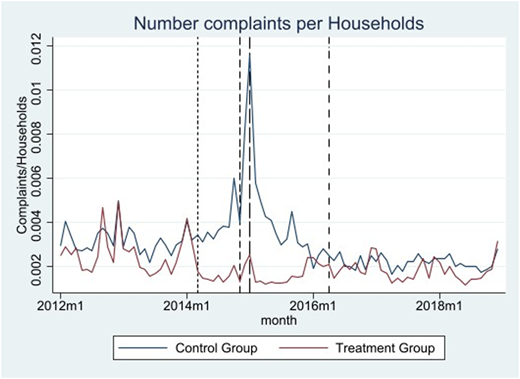
Number of water shortage complaints per household in the MRSP municipalities (treatment group) and other municipalities of the State of São Paulo (control group). Source: based on SABESP data. The first dashed vertical line marks the beginning of the Water Crisis period; the second one marks the start of the water pressure reduction in pipes; the third one marks the start of the financial burden program and the last one marks the cessation of all measures and the end of the water crisis
Number of water shortage complaints per household in the MRSP municipalities (treatment group) and other municipalities of the State of São Paulo (control group). Source: based on SABESP data. The first dashed vertical line marks the beginning of the Water Crisis period; the second one marks the start of the water pressure reduction in pipes; the third one marks the start of the financial burden program and the last one marks the cessation of all measures and the end of the water crisis
The evidence supporting that a more intense water pressure reduction in pipes began after its announcement is a significant surge in the number of water shortage complaints per household in the MRSP following the announcement. The number of water shortage complaints, which was oscillating around 3,000 complaints per month in the MRSP before November 2014, almost doubled in November (jumping to 5,727 complaints) and increased again by more than 2,000 complaints in December 2014. This surge in water shortage complaints in the MRSP is depicted in Graph 2. Even admitting that the water supply may have been restricted, at least to some extent, at some point before the announcement of the water pressure reduction (November 2014), it is quite clear that the strong negative supply shock, implemented by the reduction of water pressure, occurred after this announcement. Still, as will be seen, the monthly volume of water available for the MRSP was included as a control variable.
An increase in the number of water shortage complaints can be expected when there is a disparity between water demand and supply. This can occur due to excessive water consumption (for example, in a crowded summer resort town) or inadequate supply (as seen during the Water Crisis). In the former scenario, there should be a positive correlation between water consumption and the number of complaints: higher water consumption leads to more frequent water shortage incidents and increased complaints. In the latter case, the correlation should be negative: interruptions in the running water supply or lower water pressure in pipes result in reduced water consumption and higher water shortage complaints.
Another interesting feature of the number of water shortage complaints is that, apparently, it tends to increase suddenly in the first moment of scarcity. Even if scarcity remains, the number of complaints tends to decrease. The well-marked complaints peak right after the water pressure reduction announcement, suggests this type of consumer behavior. To smooth the path of the number of complaints per household, we used a municipal moving average of this number as a control variable in our regression models to control for the municipal degree of water scarcity over time.
3.3 The econometric models’ specification
We designed a difference-in-differences (diff-in-diff) model to assess the extent to which the reduction in water consumption during the initial months of the water crisis in the Metropolitan Region of São Paulo (MRSP) can specifically be attributed to the financial bonus program while controlling for other factors, such as the impact of the statewide public campaign, launched simultaneously to promote water consumption reduction, and for the other policies for water conservation implemented in the MRSP throughout the water crisis. Data from the residential category households were used to estimate the model parameters, aggregated at the municipal level. We estimated the following equation using the fixed effects panel data model:
The definitions of the variables are:
: Water consumption () of the municipality in month divided by the number of served households [8] within the municipality.
: dummy variable that is equal to 0 before March/2014, when the bonus program started, and 1 afterward;
: dummy variable that is equal to 0 before November/2014, when the water pressure reduction was officially announced, and 1 afterward;
: dummy variable that is equal to 0 before January/2015, when the financial burden measure was announced, and 1 afterward;
: dummy variable that is equal to 0 before April/2016, when all the previous measures were terminated, and 1 afterward;
: dummy variable that assumes the value 1 if the municipality i is one of the 38 municipalities in the MRSP and 0 otherwise.
: fixed characteristics of the municipalities (fixed effects)
: error term
: control variables vector, which will all be detailed in the next section.
Our primary interest is in coefficient β5, which measures the effect of the financial bonus program on residential water consumption.
The monthly volume of water available for the MRSP was included as a control variable. It was measured as a percentage of storage capacity and interacted with the treatment variable (Treated). By doing this, we aim to control for the fact that a more severe water shortage in the MRSP may have affected how much water SABESP could deliver to residences in this area, even as early as the beginning of 2014 as well as the impact of daily local media coverage, which may have encouraged residents to consume water more responsibly, in addition to the effect of the public campaign.
Most municipalities outside the MRSP did not experience a water crisis, and information about the water supply outside the MRSP is unavailable. As a proxy for this, we added a moving average of the monthly number of municipal water shortage complaints per household in the regressions. We used a moving average to smooth the path of the variable. The moving average includes the current complaints and the five previous ones.
We also included monthly dummies and the interaction of these dummies with the treatment variable as well as linear and quadratic time trend variables. The monthly dummy variables interacted with the dummy variable to allow for variations in the seasonal water consumption pattern between treated municipalities and the others. This difference in seasonality is supported by the two water consumption time series presented in Graph 3, in the following section.
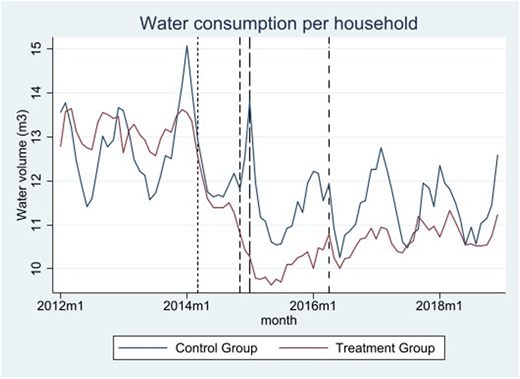
Water residential consumption, control and treatment groups, 2012m1–2018m12. Source: Based on SABESP data. The first dashed vertical line marks the beginning of the Water Crisis period; the second one marks the start of the water pressure reduction in pipes; the third one marks the start of the financial burden program and the last one marks the cessation of all measures and the end of the water crisis
Water residential consumption, control and treatment groups, 2012m1–2018m12. Source: Based on SABESP data. The first dashed vertical line marks the beginning of the Water Crisis period; the second one marks the start of the water pressure reduction in pipes; the third one marks the start of the financial burden program and the last one marks the cessation of all measures and the end of the water crisis
We are particularly interested in the coefficient , which serves as our measure of the effect of the price incentives program on water consumption, although some other coefficients specified in Equation (1) also provide valuable information. The coefficient measures the difference in the water consumption reduction between the treatment and control groups at the onset of the water crisis. If the parallel trends assumption holds and other variables influencing the water consumption are controlled, the coefficient can be interpreted as the effect of the price incentives program on water consumption in MRSP municipalities, where the bonus program was introduced. The coefficient , on the other hand, assesses the water consumption reduction at the onset of the water crisis, considering all municipalities. This reduction results, at least in part, from the statewide public campaign to reduce water consumption also initiated in March 2014. The coefficient provides information about the public campaign’s effect on reducing water consumption.
The rationale behind difference-in-differences (diff-in-diff) models is that if the event never occurs, the difference between treatment and control groups should remain consistent over time. We conducted a regression for this pre-event period to assess parallel trends before the event (water crisis). In addition to controls for seasonality, this regression included year dummy variables (time effects) and interactions between these year dummy variables and the treatment group dummy variable. Additionally, as an alternative way to account for time effects, we performed a linear time trend regression, and the time trend interacted with the treatment group dummy variable. The results are presented in the following section.
As for the other coefficients specified in Equation (1), in addition to the coefficients , we expect a negative sign for the coefficients . Coefficient informs the additional consumption reduction after the announcement of the water pressure reduction in pipes, specifically in the MRSP (that is, the difference of the variation that occurred after November 2014 between the treatment and control groups). Coefficient informs the subsequent additional consumption reduction that occurred specifically in the MRSP after January/2015 (after implementing the financial burden program). These coefficients cannot be interpreted as the pure effects of these policies, but we expect them to be negative, and they provide some information about the effect of these policies. Coefficients and were included to determine whether the average water consumption per household remained below the pre-crisis level after the end of the Water Crisis, despite the cessation of the economic incentives program in the MRSP and the end of the statewide public educational campaign.
4. Database
The Basic Sanitation Company of the State of São Paulo (SABESP) is the source of the water consumption database used in this paper. Data were collected from 362 municipalities [9] served by the company from 2012 to 2018. Water consumption information is collected every month. The selected analysis period covers two years before and after the 2014–2016 Water Crisis period [10]. We restricted our analysis to the regular “Residential” category [11].
Graph 3 shows the monthly water consumption per household from January 2012 to December 2018. Data is divided between treatment (MRSP municipalities) and control groups (other SABESP municipalities). It shows a significant reduction in water consumption starting at the beginning of 2014, as the Water Crisis broke out (dashed vertical line), a more substantial decrease in water consumption after the reduction of water pressure in pipes in November 2014 (dotted vertical line), especially for the treatment group municipalities; and a slow recovery after 2016 (dash-and-dot vertical line) when the “bonus and financial burden” program and the statewide public campaign were over.
Graph 4 shows the average household water consumption before the beginning of the water crisis in March 2014 (“Before”); after the beginning of the Water Crisis but before the reduction of the water pressure in pipes in November 2014 (“Period 1”); after the reduction of the water pressure in pipes but before the beginning of the financial burden program (“Period 2”); after the beginning of the financial burden program (“Period 3”) and after the Water Crisis (“After”). Again, the data were broken between the Treatment and Control groups. According to the graph, both groups reduced their average water consumption during the crisis and showed some stability after the crisis, but the reduction was stronger for the Treatment Group.
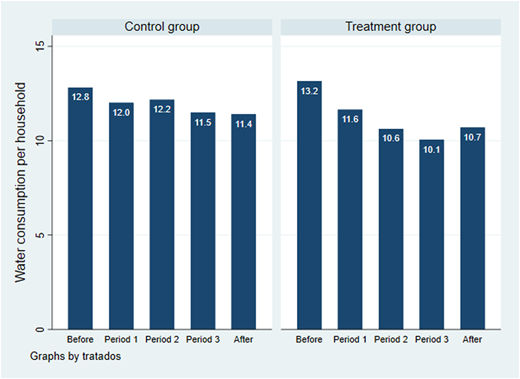
Average water consumption per household (m3): before, during and after the water crisis. Source: Based on SABESP data
Average water consumption per household (m3): before, during and after the water crisis. Source: Based on SABESP data
Our regression models included several monthly control variables: average temperature, rainy days, per capita income, population density (inhabitants per square kilometer), availability of water, a moving average of the number of water shortage complaints from consumers and linear and quadratic time trends. The source and definition of these variables can be seen in Table 2. The Bloomberg website provides information on average temperatures and rainy days. We considered days with precipitation greater than 1 mm for the latter, following Ramos et al. (2009). The source for the income information is the Fundação SEADE (State of São Paulo’s Data Analysis System Foundation). Income information is available for administrative regions within São Paulo State quarterly. Therefore, each municipality’s income was from its respective administrative region. The source of municipal areas used in the density variable was the IBGE (Brazilian Institute for Geography and Statistics) website. Data were replicated throughout the months when the information frequency was other than monthly. The company provided the monthly number of water shortage complaints in all municipalities served by SABESP.
Source of variables
| Variable | Description | Source | Original frequency |
|---|---|---|---|
| Water consumption per household (consumption_house) | The monthly total volume of water consumption divided by the number of households served in the municipality (m3/household) | SABESP | monthly |
| Temperature | Monthly average temperature (oC) | Bloomberg | daily |
| Rainy days (rainy_days) | Number of days with precipitation >1 mm in each month | Bloomberg | daily |
| Population (pop) | Number of inhabitants in a municipality | IBGE | annual |
| Per capita income (income_cap) | Quarterly São Paulo’s Administrative Regions GDP divided by the population | Fundação SEADE | quarterly |
| Density | A population divided by the total municipality area | IBGE | annual |
| Water shortage complaints (complain) | Number of water shortage complaints divided by the number of households in a municipality | Sabesp | monthly |
| Monthly volume of water available at Cantareira System (vol_Cant_pc) | Percentage of storage capacity at SABESP’s Cantareira System reservoir | Sabesp | monthly |
Source(s): Authors’ elaboration
Table 3 shows descriptive statistics for the data used in the regression Model 1, categorized into Treatment and Control groups. The mean water consumption per household in the control group was 12.02, whereas in the treatment group it was 10.99. The average temperatures and rainy days were similar in both groups. The Treatment group exhibited significantly higher population, density and income per capita values, indicating greater urbanization than the Control group. The maximum income per capita in both groups is the same because this variable is based on data from administrative regions that may encompass municipalities in both groups. Finally, “complaints per household” is higher in the Treatment group than in the Control group.
Descriptive statistics of variables
| Variable | Obs | Mean | Standard dev | Minimum | Maximum |
|---|---|---|---|---|---|
| Total | |||||
| Water consumption per household (consumption_h) | 30,735 | 11.90 | 1.650 | 4.301 | 26.95 |
| Temperature | 30,479 | 22.58 | 3.025 | 11.43 | 30.33 |
| Rainy days (rainy_days) | 30,479 | 10.92 | 6.453 | 0 | 31 |
| Population ‘000 (pop) | 30,735 | 205.07 | 1,381 | 0.81 | 12176.87 |
| Per Capita Income (income_cap) | 30,735 | 8,615 | 2,606 | 3,272 | 15,538 |
| Density | 30,735 | 447.4 | 1,576 | 0.16 | 14,007 |
| Water shortage complaints per household (complaint) | 30,735 | 0.0019 | 0.0036 | 0.000 | 0.080 |
| Volume of water available at Cantareira System (vol_Cant_pc) | 30,735 | 35.04 | 29.44 | −24.3 | 76.4 |
| Control group | |||||
| Water consumption per household (consumption_h) | 27,215 | 12.02 | 1.63 | 4.30 | 26.95 |
| Temperature | 26,979 | 22.77 | 3.02 | 11.43 | 30.33 |
| Rainy days (rainy_days) | 26,979 | 10.81 | 6.44 | 0.00 | 31.00 |
| Population ‘000 (pop) | 27,215 | 29 | 64.81 | 0.81 | 713.94 |
| Per capita income (income_cap) | 27,215 | 8,071 | 2,211 | 3,272 | 15,538 |
| Density | 27,215 | 112.2 | 358.5 | 0.16 | 3,642.5 |
| Water shortage complaints per household (complaint) | 27,215 | 0.001 | 0.003 | 0.000 | 0.080 |
| Volume of water available at Cantareira System (vol_Cant_pc) | 27,215 | 35.04 | 29.44 | −24.3 | 76.4 |
| Treatment group | |||||
| Water consumption per household (consumption_h) | 3,520 | 10.99 | 1.56 | 8.04 | 18.26 |
| Temperature | 3,500 | 21.05 | 2.62 | 13.69 | 26.71 |
| Rainy days (rainy_days) | 3,500 | 11.81 | 6.48 | 0.00 | 31.00 |
| Population ‘000 (pop) | 3,520 | 1568.28 | 3812.53 | 5.81 | 12176.87 |
| Per capita income (income_cap) | 3,520 | 12,823 | 1,222 | 9,549 | 15,538 |
| Density | 3,520 | 3039.0 | 3620.0 | 32.0 | 14006.8 |
| Water shortage complaints per household (complaint) | 3,520 | 0.005 | 0.006 | 0.000 | 0.074 |
| Volume of water available at Cantareira System (vol_Cant_pc) | 3,520 | 35.04 | 29.44 | −24.3 | 76.4 |
Source(s): Based on SABESP, Bloomberg, Fundação SEADE and IBGE data
We ran a regression for the period before the Water Crisis, including yearly dummy variables (time effects) alone and interacted with the Treatment group dummy variable to test for parallel trends between the Treatment and Control groups. As an alternative way to control time effects, we ran a regression that included a linear time trend, and the time trend interacted with the treatment group dummy variable. Both regressions included monthly dummy variables and the interaction of these dummies with the treatment dummy to control seasonality. The results of these regressions are presented in Table 4.
Tests for parallel trends: Dependent variable = average monthly household water consumption by municipality
| Regression using year dummies | |
| Treatment dummy | −0.65307*** (−3.49) |
| Year dummy 2012 | 0.05792* (1.65) |
| Year dummy 2014 | 1.06609*** (13.90) |
| Year dummy 2012 interacted with Treatment group dummy | 0.01455 (0.14) |
| Year dummy 2014 interacted with the Treatment group dummy | −0.31907 (−1.41) |
| Regression using linear time trend | |
| Treatment dummy | −0.52279** (−2.35) |
| Linear trend | 0.01599*** (6.62) |
| Linear trend interacted with the Treatment group dummy | −0.00683 (−0.95) |
Note(s): (1) Regressions estimated for the period before the Water Crisis (from January 2012 to February 2014); (2) Regressions include dummies for months and the interaction of these dummies with the treatment dummy variable. In both cases, the coefficients were statistically significant and (3) t statistics in parentheses; *p < 0.10, **p < 0.05 and ***p < 0.01
Source(s): Authors’ elaboration
The coefficients for the interactions between the yearly dummy variables and the Treatment group dummy variables were not statistically significant, indicating that the two groups did not have different trends over time during this period and the parallel trends assumption was not violated. This was also the case with the coefficient for the linear time trend interacted with the Treatment group dummy variable, further confirming that the parallel trends assumption was not violated.
Graph 5 in the Appendix shows the two series of average household consumption (treatment and control groups), where we filtered out the seasonal component from each series. The graph illustrates a parallel movement of the two series before March 2014 and a shift afterward, including a point where the two series intersect.
5. Results
This section presents and discusses the results of the estimations of equation (1), as defined in Section 3. Table 5 displays these results, progressively incorporating control variables up to the fifth regression, which includes all of them.
Econometric model results (average monthly household water consumption by municipality)
| (1) | (2) | (3) | (4) | (5) | (6) | |
|---|---|---|---|---|---|---|
| after1 | −0.479*** | −0.661*** | −0.512*** | −0.488*** | −0.592*** | −0.609*** |
| (−24.02) | (−28.57) | (−20.60) | (−19.39) | (−22.81) | (−24.84) | |
| after2 | −0.448*** | −0.487*** | −0.615*** | −0.659*** | −0.681*** | −0.687*** |
| (−15.53) | (−16.21) | (−21.48) | (−24.26) | (−25.19) | (−27.07) | |
| after3 | −0.464*** | −0.502*** | −0.354*** | −0.330*** | −0.312*** | −0.319*** |
| (−20.85) | (−22.14) | (−17.21) | (−16.59) | (−15.93) | (−15.95) | |
| after4 | 0.184*** | 0.239*** | 0.233*** | 0.244*** | 0.395*** | 0.376*** |
| (11.85) | (13.28) | (12.54) | (13.23) | (17.29) | (17.05) | |
| after1_treated | −0.726*** | −0.650*** | −0.657*** | −0.862*** | −0.532*** | −0.534*** |
| (−12.20) | (−11.49) | (−11.71) | (−14.64) | (−10.48) | (−10.72) | |
| after2_treated | −0.952*** | −0.941*** | −0.954*** | −0.553*** | −0.490*** | −0.486*** |
| (−14.38) | (−14.24) | (−13.85) | (−9.11) | (−7.91) | (−7.97) | |
| after3_treated | 0.0202 | 0.0349 | 0.0583 | −0.140* | −0.153** | −0.155** |
| (0.38) | (0.66) | (1.08) | (−2.45) | (−2.68) | (−2.75) | |
| after4_treated | 0.535*** | 0.574*** | 0.571*** | 0.503*** | 0.158* | 0.116 |
| (11.58) | (11.76) | (12.05) | (11.30) | (2.05) | (1.80) | |
| Temperature | 0.261*** | 0.259*** | 0.222*** | 0.224*** | 0.224*** | 0.221*** |
| (43.79) | (42.17) | (28.07) | (27.19) | (27.15) | (25.44) | |
| rain_days | −0.0155*** | −0.0147*** | −0.0306*** | −0.0307*** | −0.0307*** | −0.0301*** |
| (−10.66) | (−10.24) | (−13.15) | (−13.35) | (−13.33) | (−15.42) | |
| renda_cap_000 | 0.0821*** | 0.0612*** | 0.00168 | 0.0108 | 0.00926 | 0.0199 |
| (6.16) | (4.46) | (0.12) | (0.76) | (0.65) | (1.42) | |
| density_000 | −0.420 | 0.456 | 0.448 | 0.516* | 0.574* | 0.629** |
| (−1.27) | (1.75) | (1.76) | (2.05) | (2.26) | (2.66) | |
| pop_mi | −28.14*** | −26.28*** | −25.92*** | −25.32*** | −22.42*** | |
| (−4.03) | (−3.86) | (−3.81) | (−3.72) | (−3.43) | ||
| pop2_bi | 0.00114*** | 0.00106*** | 0.00105*** | 0.00103*** | 0.000902** | |
| (3.92) | (3.74) | (3.70) | (3.61) | (3.31) | ||
| Tempo | 0.0209*** | 0.0196*** | 0.0187*** | 0.0159*** | 0.0182*** | |
| (10.11) | (8.98) | (8.53) | (7.21) | (8.76) | ||
| tempo2 | −0.000192*** | −0.000178*** | −0.000174*** | −0.000153*** | −0.000173*** | |
| (−12.34) | (−11.17) | (−10.86) | (−9.48) | (−10.86) | ||
| vol_Cant_pc | −0.00246*** | −0.00235*** | ||||
| (−6.74) | (−6.42) | |||||
| vol_Cant_pc_treated | 0.00596*** | 0.00653*** | ||||
| (6.10) | (7.69) | |||||
| moveave_recl | 1.015 | |||||
| (0.27) | ||||||
| N | 30,479 | 30,479 | 30,479 | 30,479 | 30,479 | 28,659 |
| R2 | 0.608 | 0.615 | 0.640 | 0.647 | 0.647 | 0.677 |
| adj. R2 | 0.608 | 0.614 | 0.640 | 0.646 | 0.647 | 0.676 |
Note(s): Errors clustered at municipal level; t statistics in parentheses: *p < 0.05, **p < 0.01 and ***p < 0.001
Source(s): Based on SABESP, Bloomberg, Fundação SEADE and IBGE data
Starting from the period before the water crisis, the estimated coefficients indicate a significant reduction in water consumption per household after the onset of the water crisis, after the announcement of the water pressure reduction in the MRSP pipelines and after implementing the financial burden program in the MRSP.
The coefficients for the interaction term are the primary focus of this study, as they represent the impact of the price incentives program on water consumption. These coefficients were consistently significant at the 1% level and negative across all regressions. In the first column, the coefficient was −0.726; in the fourth and fifth columns, the coefficients were −0.532 and −0.534. The fourth regression included the water volume available for the MRSP, which also interacted with the treatment variable, and the fifth regression included the moving average of the municipal number of water shortage complaints per household.
Since the parallel trends assumption holds, and the effects of the rise of water scarcity at the onset of the water crisis are controlled, the coefficient for the interaction term can be interpreted as the effect of the price incentives program, which was introduced only in the municipalities of the MRSP. This is because the coefficient for the After1 variable quantifies the decline in water consumption at the onset of the water crisis that occurred in all municipalities served by SABESP.
In other words, during the first eight months of the Water Crisis, the population in the MRSP made an additional effort to reduce water consumption per household compared to the control group. This extra effort can be attributed to the price incentives program, which was already in operation during this period, while a significant water pressure reduction in pipes had yet to occur. Our coefficients indicate that, at the onset of the water crisis, after the initiation of the price incentives program and the statewide public campaign, the population in the MRSP decreased monthly water consumption by an average of approximately 1.14 m3 (sum of and coefficients) compared to the pre-Water Crisis period. This reduction was 0.53 m3 greater than the control group’s average consumption reduction during the same period [12]. For comparison, the coefficient for the consumption reduction in the MRSP in Souza and Fouto (2019) was −1.589. Nevertheless, their study did not have a control group not submitted to the price incentives program.
On the other hand, Grover and Lucinda (2020) specified a control group to measure the effect of the financial bonus program. The control group consisted of households in the city of São Paulo that were not served by the Cantareira reservoir, and therefore, were not eligible for the bonus program during the first two months following its implementation. After these two months, all households in the MRSP became eligible. This brief period might explain why the authors found no effect associated with the bonus program, since households participating in the bonus program may not have had sufficient time to adjust to the new incentives within two months.
It is interesting that residential water consumption consistently declined during the water crisis even in municipalities outside the MRSP, since the estimated coefficients for After1, After2 and After3 were all negative and statistically significant at the 1% level. They suggest that the campaign and the “awareness effect” were also effective even in the municipalities that did not experience a water crisis, which was the case for almost all the municipalities outside the MRSP.
The coefficients for the interaction term are also consistently negative and significant at the 1% level in all regressions, strongly suggesting that water pressure reduction in the MRSP pipelines had a substantial impact. After the water pressure reduction announcement, we observed an additional decline in water consumption, which was more pronounced in the MRSP. The monthly water consumption in the treatment group declined by approximately 0.49 m3 more on average in comparison to the control group (see Table 5, fifth column). This coefficient provides some evidence of the magnitude of the effect of the water pressure reduction, suggesting that it was similar to the impact of the price incentives program. The coefficients for the interaction terms and shown in the fifth column of Table 5 were tested, and we found out that they are statistically equal.
The coefficients for the interaction term are negative in the last three regressions of Table 5 and significant at the 5% level in the last two regressions, suggesting that the financial burden program had a negative effect on consumption. After the implementation of the burden program in the MRSP, we observe again an additional fall in water consumption, which was more pronounced in the MRSP, but this difference between treatment and control groups was smaller than the one observed right after the water pressure reduction. After January 2015, monthly water consumption in the MRSP declined by approximately 0.15 m3 more on average in comparison to the control group (see Table 5, fifth column), providing some evidence that the financial burden program impacted the water consumption, although weaker than the impact of the price incentives program.
The coefficients estimated for the dummy variable are positive and significant at a 1% level in all regressions, meaning that the water consumption increased after the water conservation policies adopted in the MRSP and the statewide public campaign ended, but it did not return to the pre-crisis level. Considering the coefficients in the fifth column, we observe that after March/2016 monthly water consumption per household increased by approximately 0.38 m3 on average in comparison to the previous period (between January/2015 and March/2016), when the public campaign was still in progress as well as the other policies implemented in the MRSP. Nevertheless, the total decrease in monthly water consumption per household during the crisis for the control group was approximately 1.98 m3 on average. That is, the average water consumption per household after the crisis stayed far below the pre-crisis level, at least until December/2018, suggesting long-term effects. Households may have been encouraged to invest in water tanks, water-saving toilets and long-run behavioral changes regarding water consumption.
The results also indicate that this eventual long-term effect was more substantial in the MRSP, as expected, since the total fall in water consumption during the water crisis was more pronounced in this region, and the rise after the crisis in the MRSP was similar to the rise observed in the control group. The coefficients for the interaction term are positive, but in the fifth regression, this coefficient is not statistically significant (approximately 0.12).
Regarding the control variables, coefficients for the monthly water volume available at the Cantareira System were positive for the treatment group, as expected (see section 3), and statistically significant at the 1% level. That is, a fall in water availability for the MRSP is related to a fall in water consumption in this region. Considering the fifth column of Table 5, we observe that a raise of one percentage point in the volume of water available at the Cantareira System (measured as a percentage of storage capacity) is related to a raise of approximately 0.0042 m3 (sum of Vol_cant_pc and Vol_cant_pc_treated coefficients) in monthly water consumption per household in the MRSP. The coefficient for the moving average of the municipal number of water shortage complaints per household was not statistically significant.
The coefficients for temperature were positive and negative for rainy days (Martinez-Espineira, 2002). Demographic variables such as population and squared population were statistically significant in all regressions, while coefficients for the population density were not. Per capita income coefficients were statistically significant only in the first two regressions. The income elasticity of water consumption in high-income households tends to be small (Arbués, García-Valiñas, & Martínez-Espiñera, 2003) since water expenditure is usually a tiny share of the household expenditure (only 0.94%, according to the 2017–2018 IBGE Household Budget Survey). Both Souza et al. (2021) and Andrade, Brandão, Lobão, and Silva (1995) also found very small coefficients for the income effect on water consumption, although significant [13].
6. Conclusions
From 2014 to 2016, the Metropolitan Region of São Paulo (MRSP), Brazil, experienced a severe water shortage, during which the water services state provider (São Paulo State Basic Sanitation Company – SABESP) adopted a price incentives program and a solid public campaign for water consumption reduction. The price incentives program covered over 17 million people in 31 municipalities of the Metropolitan Region of São Paulo (MRSP), while the public campaign was statewide. A few months later, SABESP also announced additional policies, like a reduction in water pressure in the MRSP’s pipelines (eight months later) and a financial burden program (10 months later).
This study tested the causal relationship between the price incentives program, implemented exclusively in the MRSP and residential water demand after controlling for other factors. The study also evaluates the decline in water consumption after the announcement of additional policies, such as the water pressure reduction in the MRSP’s pipelines and the financial burden. We also evaluated whether water consumption remained low or returned to the pre-crisis level. Price and non-price incentives may have hypothetically encouraged household investments in water savings, water tanks, toilets and once-for-all long-run behavior changes.
We adopted a diff-in-diff methodology using a fixed-effects panel data model comparing the municipalities of the MRSP, where the economic incentives program was adopted, with the other cities served by the same state company.
Our results demonstrate a significant decrease in water consumption in all municipalities during the initial months of the water crisis. This reduction was more pronounced in the MRSP than in the other cities, which were also submitted to the public campaign (but not to economic incentive programs), even though the water crisis did not happen or was considerably softer in these cities. After controlling for many factors, we found that, on average, the price incentives program reduced monthly water consumption by approximately 0.5 m3 per household. We also provided evidence that the effect associated with the water pressure reduction in the MRSP’s pipelines was similar. At the same time, the impact of the financial burden program appears to have been weaker. Souza and Fouto (2019) also estimated a significant effect of the price incentives program, but at a higher level. Grover and Lucinda (2020) found no impact associated with this program and a significant impact related to the financial burden program. We pointed out that the control group used by Grover and Lucinda (2020) could lead to an underestimate of the effect of the bonus program on water consumption.
Finally, it is worth noting that after the crisis, when all the adopted policies had concluded, water consumption remained lower than pre-crisis levels in all municipalities. This suggests that the combination of price and non-price incentives encouraged households to make long-lasting investments in water-saving practices.
Price and non-price incentives to reduce water consumption can also have varying impacts on different consumer groups. Investigating the distribution of the burden of a water-saving program is an important issue that warrants further research, but it falls outside the scope of the present study.
The authors would like to express their gratitude to the anonymous referees, whose suggestions greatly contributed to the development of our paper.
Notes
“Low-income households were found to be more than five times as price responsive as relatively wealthy households reflecting the fact that their water bill typically constitutes a larger share of the household budget” (Renwick & Archibald (1998, p. 357).
“If water demand management occurs solely through price increases, low-income households will contribute a greater fraction of a city’s aggregate water savings than high income households, in part because price elasticity declines with the fraction of household income spent on a particular good. The empirical evidence supports this conclusion. (…) But the distributional impact of most nonprice programs depends on how they are financed”. Olmstead and Stavins (2009, p. 5).
“… there was a significant reduction in water consumption in the MRSP, Brazil, subsequent to the 2013–2015 drought; almost 5 years after the worst moment of scarcity, the population did not return to its consumption threshold before the implementation of the bonus and financial burden. Evidence indicates that there was resilience built during the crisis in response to the water scarcity, which led to the adoption of new water consumption practices” (Souza et al., 2021, p. 12).
See details in Section 4.
The DiD is a well-known double difference method. The treatment effect can also be assessed using a fixed-effects model for panel data, which controls for all characteristics that are fixed over time for each municipality, thereby significantly reducing the likelihood of omission bias in the estimators.
Technically, “households” refers to “economies,” which are defined as a numbered property or a numbered subdivision of a property, taken as the unit of consumption. It can be a house, a building, or an apartment inside a building.
See Appendix for the complete list of municipalities.
We analyzed each municipal data individually; we corrected 28 observations that showed clearly mistyped data in the original database, either by interpolation or by dividing/multiplying by 10 or 100.
Besides the regular “Residential” category, there are two additional residential categories within SABESP’s tariff structure: the “Social-Residential” category for low-income households, and the “Slum-Residential” category, for those who live in irregular areas. Tariffs in the Social-Residential category are significantly lower than those in the regular “Residential” category (see Appendix). The “Slums-Residential” category water consumption tariff is even lower. We opted to restrict our analysis to the regular residential category because the “Slums-Residential” category encompasses only few households in many municipalities, and the analysis of the “Social-Residential” category did not meet the test for parallel trends.
As a robustness test, we ran a regression including a specific nonlinear time trend for the crisis period as well as a regression including observations just until October/2014. Our estimation of the effect of the price incentives program remained stable.
The monthly dummy variables included to control seasonality were statistically significant, including the ones interacted with the control group dummy variable, confirming that the seasonal pattern of water consumption is different for treatment and control groups.
Conflict of interest statement: The author Leonardo Poyo Chen reports having an employment relationship with SABESP while the dissertation paper on which this paper is based was elaborated.
Data access statement: Data supporting this study cannot be made available due to legal or commercial restrictions.
Ethics statement: All authors contributed to the work’s development, critical revision and final approval and agree to accept responsibility for it.
Funding statement: This research received no specific grant from any funding agency in the public, commercial or not-for-profit sectors.
References
Further reading
The supplementary material for this article can be found online.

