
This study aims to assess the use of variational quantum imaginary time evolution for solving partial differential equations using real-amplitude ansätze with full circular entangling layers. A graphical mapping technique for encoding impulse functions is also proposed.
The Smoluchowski equation, including the Derjaguin–Landau–Verwey–Overbeek potential energy, is solved to simulate colloidal deposition on a planar wall. The performance of different types of entangling layers and over-parameterization is evaluated.
Colloidal transport can be modelled adequately with variational quantum simulations. Full circular entangling layers with real-amplitude ansätze lead to higher-fidelity solutions. In most cases, the proposed graphical mapping technique requires only a single bit-flip with a parametric gate. Over-parameterization is necessary to satisfy certain physical boundary conditions, and higher-order time-stepping reduces norm errors.
Variational quantum simulation can solve partial differential equations using near-term quantum devices. The proposed graphical mapping technique could potentially aid quantum simulations for certain applications.
This study shows a concrete application of variational quantum simulation methods in solving practically relevant partial differential equations. It also provides insight into the performance of different types of entangling layers and over-parameterization. The proposed graphical mapping technique could be valuable for quantum simulation implementations. The findings contribute to the growing body of research on using variational quantum simulations for solving partial differential equations.
1. Introduction
Partial differential equations (PDEs) are fundamental to solving important problems in engineering and science. With the advent of nascent quantum computers, finding new efficient quantum algorithms and hardware for solving PDEs has become an active area of research (Tosti Balducci et al., 2022; Jin et al., 2022; Leong et al., 2022; Pool et al., 2022) in disciplines ranging from fluid dynamics (Budinski, 2021; Gaitan, 2020; Steijl, 2022; Steijl and Barakos, 2018; Griffin et al., 2019; Li et al., 2023), heat conduction (Liu et al., 2022) and electromagnetics (Ewe et al., 2022) to quantitative finance (Fontanela et al., 2021) and cosmology (Mocz and Szasz, 2021).
Although linear differential equations can be solved by the quantum linear solver algorithm (Berry et al., 2017; Harrow et al., 2009), the required resources are out of reach of the current noisy intermediate-scale quantum devices (Lau et al., 2022; Bharti et al., 2022; Preskill, 2018). In fact, practical near-term quantum algorithms are limited to those designed for short circuit depths, such as variational quantum algorithms (VQAs) (Cerezo et al., 2021), which use parameterized ansätze to optimize cost functions via variational updating.
VQAs can largely be classified into two categories, namely, optimization and simulation (Endo et al., 2021), each offering unique approaches to solving PDEs. Variational quantum optimization (VQO) aims to optimize a static target cost function through parameter tuning, an example of which is the popular variational quantum eigensolver (VQE) (Peruzzo et al., 2014) for minimizing energy states in the field of quantum chemistry. This led to the development of the variational quantum linear equation solver (Bravo-Prieto et al., 2019; Huang et al., 2021; Xu et al., 2021) for systems of linear equations and the variational quantum Poisson solver (Liu et al., 2021; Sato et al., 2021). Evolution of the Poisson equation allows parabolic PDEs to be solved through implicit time-stepping (Leong et al., 2022), which requires quantum information to be updated and encoded at each time-step.
On the other hand, variational quantum simulation (VQS) aims to simulate a dynamical quantum process, such as the Schrödinger time evolution (Li and Benjamin, 2017). This allows certain PDEs to be solved efficiently using imaginary quantum time evolution (Endo et al., 2021; Endo et al., 2020; Yuan et al., 2019), including the Black–Scholes equation for option pricing (Miyamoto and Kubo, 2021; Radha, 2021; Stamatopoulos et al., 2020) and stochastic differential equations for stochastic processes (Kubo et al., 2021). Recent work on the Feynman–Kac formulation (Alghassi et al., 2022) generalizes quantum simulation of parabolic PDEs, paving the way for potential near-term applications.
In this study, we explore applications of VQS (Miyamoto and Kubo, 2021; Alghassi et al., 2022) in solving PDEs, including the Smoluchowski equation for colloidal physics, with an emphasis on potential and non-homogeneous terms oft-neglected in quantum simulations. We select for high-fidelity real-amplitude ansätze, assess time complexity and propose an efficient encoding scheme for idealized pulse functions, as a proof of concept towards practical implementation of quantum simulation.
2. Variational quantum simulation
2.1 Evolution equation
Consider a 1-dimensional (1D) evolution equation expressed in the Feynman–Kac formulation (Alghassi et al., 2022):
where u(t) = u(x, t) is a function of space x and time t, and a, b and c are the coefficients to the second-, first- and zeroth-order derivative terms in x, respectively (bold symbols denote vectors in space x). f (t) = f (x, t) is a non-homogeneous source term and u0 is the initial condition. Following (Kubo et al., 2021), we rewrite equation (1) in Dirac notation [1]:
where (t): = a∂xx + b∂x + c is the Hamiltonian operator, possibly non-Hermitian, and (t) is a linear operator satisfying (t)|0〉 = |f(t)〉. The non-homogeneous operator (t) can be expressed as a sum of unitaries. Using VQS (McArdle et al., 2019), the state |u(t)〉 can be approximated by an unnormalized trial state formed by a set of parameterized unitaries {Rk}k∈[N] with N parameters:
where θ0(t) is a normalization parameter. To minimize the distance , we apply the McLachlan’s variational principle (Yuan et al., 2019):
where denotes the Euclidean norm and δ denotes infinitesimal variation. This yields a system of ordinary differential equations:
where . The left-hand side matrix:
and the right-hand side vector:
can be evaluated parametrically on quantum circuits (McArdle et al., 2019). See Appendix 1 for details.
With A and C specified, parameters θ are evolved in time using the forward Euler method as:
up to Nt time-steps in each Δt. Higher-order methods, such as Runge–Kutta, are also available. Because the matrix A may be ill-conditioned, successful inversion may depend on methods such as the Moore–Penrose inverse or Tikhonov regularization (McArdle et al., 2019). We find that least-squares minimization with a 10−6 cutoff is sufficient for stable solutions (Fontanela et al., 2021).
2.2 Decomposition of Hamiltonian
The Hamiltonian operator introduced in equation (2) can be simplified through elimination of the skew-Hermitian term ∂x using substitution methods (Fontanela et al., 2021), such as u(t) = egv(t), where g is a function of and . If g(a, b) were constant in time, then the Hamiltonian operator reduces to Alghassi et al. (2022):
where is the identity operator. The potential vector is:
where the last term can be neglected if {} is independent of x. The Hamiltonian operator can be discretized in the space interval Δx, and decomposed into a linear combination of terms as:
where 1 = (1, 1, …, 1, 1) is the all-ones vector and . For the Neumann boundary condition, all six terms {H1, …, H6} are required. For the periodic boundary condition, only the first four terms {H1, …, H4} are required, and for the Dirichlet boundary condition, the first five terms {H1, …, H5} are required. Note that as an observable in the first term, the potential vector φ does not increase the quantum complexity; measurement of the existing H1 suffices to evaluate the expectation value of the potential.
The operator S denotes the n-qubit cyclic shift operator (Sato et al., 2021):
which can be implemented as a product of k-qubit Toffoli gates, for k in the range 1, …, n (see e.g. Sato et al., 2021, Figure 2).
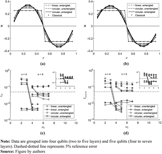
Initial step evolves under (a) periodic and (b) Dirichlet boundary condition on a 2n = 16 grid for a real-amplitude ansatz with four layers using time-step Δt = 10−4 plotted in increments of 2 × 10⁻³; mean (c) trace and (d) norm error plotted on a semi-log scale against the number of ansatz layers for various real-amplitude designs under periodic (open symbols) and Dirichlet (closed symbols) boundary conditions up to T = 10−2 (insets show peak error)
Initial step evolves under (a) periodic and (b) Dirichlet boundary condition on a 2n = 16 grid for a real-amplitude ansatz with four layers using time-step Δt = 10−4 plotted in increments of 2 × 10⁻³; mean (c) trace and (d) norm error plotted on a semi-log scale against the number of ansatz layers for various real-amplitude designs under periodic (open symbols) and Dirichlet (closed symbols) boundary conditions up to T = 10−2 (insets show peak error)
2.3 Ansatz selection
For optimal algorithmic performance, a good choice of ansatz is crucial (Tilly et al., 2022; You et al., 2021). For PDEs that admit only real solutions, it is preferable to use a real-amplitude ansatz formed by nl repeating blocks, each one consisting of a parameterized layer with one RY rotation gate on each qubit, followed by an entangling layer with CNOT gates between consecutive qubits (Alghassi et al., 2022). Here, we consider two options for customization: the first between linear and circular entanglement and the second with or without an unentangled parameterized layer as the final block nl, as shown in Figure 1.
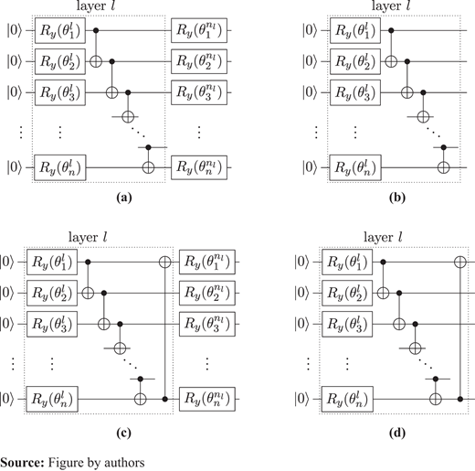
Real-amplitude ansatz formed by repeating parameterized blocks with either linear (a, b) or circular (c, d) entanglement. (a, c): Final layer nl is unentangled. (d): This full circular ansatz outperforms the other ansätze and is used throughout the study
Real-amplitude ansatz formed by repeating parameterized blocks with either linear (a, b) or circular (c, d) entanglement. (a, c): Final layer nl is unentangled. (d): This full circular ansatz outperforms the other ansätze and is used throughout the study
We note that the circular entanglement with a final unentangled layer [Figure 1(c)] is a popular choice of an ansatz for VQS (Kubo et al., 2021; Alghassi et al., 2022). For benchmarking, we perform numerical experiments on the various ansätze (Figure 1) to solve a simple 1D heat or diffusion equation, expressed in Dirac notation as:
in space x ∈ [0, 1] and time t ∈ [0, T].
The initial trial state is set as a reverse step function (Sato et al., 2021):
which can be implemented in practice by setting the final parameterized layer l as with entanglement, or without. Figure 2(a) and 2(b) show the time evolution of the step function for four-qubit real-amplitude ansätze with four layers using time-step Δt = 10−4 up to T = 10−2.
We measure the fidelity of the VQS solution obtained from each ansatz compared to the classical solution and define the trace error as:
Similarly, we define the norm error as:
where θ0(t) is the normalization parameter as previously defined. Figure 2(c) and (d) shows the mean trace and norm errors depending on the number of ansatz layers nl using time-step Δt = 10−4 up to T = 0.01, for periodic and Dirichlet boundary condition, the latter shown as closed symbols for |f(t)〉 = 0.
The circular, fully entangled ansatz [Figure 1(d)], here termed full circular ansatz for short, was found to outperform other ansätze, requiring fewer parameters for the same solution fidelity. For four qubits, the full circular ansatz is the only one able to produce a solution overlap with only two or three layers, which is less than the minimum required for convergence nl < 2n/n. For five qubits, it delivered reduced solution and norm errors compared to other ansätze, independent of the number of layers. In this benchmark, the additional term introduced by the Dirichlet boundary condition does not diminish the superior performance of the full circular ansatz.
2.4 Initialization
An initial quantum state |u(0)〉 can be prepared through classical optimization and accepting converged solutions whose norms fall below a specified threshold (Fontanela et al., 2021; Alghassi et al., 2022) or direct encoding using quantum generative adversarial networks (Zoufal et al., 2019). In most cases, quantum encoding is cost-prohibitive, and sub-exponential encoding can be achieved only under limiting conditions (Nakaji et al., 2022; Mitsuda et al., 2022).
The Dirac delta function is a popular initial probability distribution found in Fokker–Planck equations (Kubo et al., 2021; Alghassi et al., 2022). To encode the state |x〉 in the computational basis with xi ∈ {0, 1}, one seeks a parameterized ansatz for an input state |0〉.
It turns out that for a full circular ansatz [Figure 1(d)], encoding |x〉 does not necessarily require costly optimization. To access a given state |x〉, one can search for a parameterized layer nl – k such that a π bit-flip rotation on an gate (or gates) yields an input state |x0〉, which transforms to the output state after k circular entangling layers, i.e. , where the matrix Cn represents a single circular entangling layer ( Appendix 2).
Figure 3 shows that for a four-qubit full circular ansatz, all 24 – 1 = 15 |x〉 states can be encoded by a single π bit-flip rotation of an Ry gate within four parameterized layers.
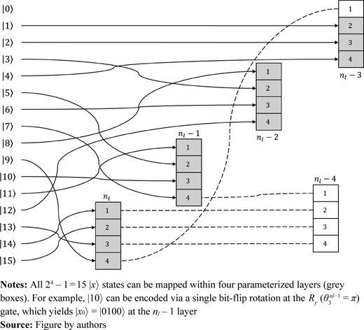
Mapping state |x〉 to an input state |x0〉 at the nl – k layer of a four-qubit full circular ansatz
Mapping state |x〉 to an input state |x0〉 at the nl – k layer of a four-qubit full circular ansatz
2.5 Time complexity
To assess the time complexity of the VQS algorithm, we estimate the number of quantum circuits required per time-step as:
where np is the number of ansatz parameters (np = nln for a real-amplitude ansatz) and nh is the number of terms in the Hamiltonian [equation (11)]. Likewise, the number of circuits required per time-step for a VQE implementation (Leong et al., 2022) can be estimated as:
where nit is the number of iterations taken by the classical optimizer. Hence, the VQS algorithm is comparable with VQE in terms of circuit counts, if the number of ansatz parameters is roughly double the expected number of iterations required for VQE, i.e. np ≈ 2nit ≫ nh.
For each circuit, the time complexity scales as (Sato et al., 2021):
where dansatz ∼ (nl) is the depth of the ansatz, dshift ∼ (n2) is the depth of the shift operator, and the denominator (ε2) reflects the number of shots required for estimated expectation values up to a mean squared error of ε2. Another consideration is the depth for amplitude encoding denc, which can range from (n2) to (2n). For VQS, encoding is performed once during initialization, but unlike VQE, repeated encoding is not necessary for time-stepping (Leong et al., 2022).
To solve an evolution PDE [e.g. equation (1)], a classical algorithm iterates a matrix of size 2n × 2n, compared to a np × np matrix for VQS, suggesting comparable performance at nl ≈ 2n/n.
3. Colloidal transport
With the VQS framework in place, one can explore applications in solving PDEs, such as heat, Black–Scholes and Fokker–Planck equations listed in Alghassi et al. (2022). In this study, we focus on colloidal transport as an application of choice, as the governing Smoluchowski equation involves deep interaction potential energy wells which can be modelled as a component of the Hamiltonian operator [equation (9)], an aspect oft-neglected in quantum simulations.
3.1 Smoluchowski equation
Consider a spherical colloidal particle of radius a near a planar wall (Torres-Díaz et al., 2019). The generalized Smoluchowski equation (Smoluchowski, 1916) describes the probability p(h, t) of locating the particle at h, the distance of the particle centre from the wall at time t, as:
where D is the diffusivity matrix. U(h) is the Derjaguin–Landau–Verwey–Overbeek (DLVO) sphere-wall interaction energy (Bhattacharjee et al., 1998), which is the sum of the electric double-layer and van der Waal’s interaction energies, expressed as:
where U = U(h) and H = (h – a)/a is the dimensionless separation distance between the particle and wall. The electric double-layer coefficient, normalized inverse Debye length and van der Waal’s coefficient are, respectively:
where ε is the relative permittivity of the medium, ε0 is the permittivity of free space, zv is the ionic valence, e is the electron charge, kB is the Boltzmann’s constant and T is the temperature. ζp and ζw are the zeta potentials on the colloidal particle and wall, respectively. I is the ionic strength and AH is the Hamaker constant.
With that, the first and second derivatives of the interaction energy in separation distance are:
Rescaling time τ = tD/a2, we rewrite equation (20) in dimensionless form, which gives the evolution of the probability p(τ) = p(H, τ) as:
which follows from equation (1), where = 1, = U′, = U″ and = 0. Suitable boundary conditions are the absorbing condition on the surface at p(0) = 0 (Dirichlet) and the no-flux condition in the far field ∂p(∞)/∂H → 0 (Neumann) (Torres-Díaz et al., 2019).
Substituting p(τ) = ρ(τ)e–U/2 (Fontanela et al., 2021), we express in Dirac notation:
with the Hamiltonian operator:
and the potential term:
which can be evaluated classically [equation (23)] and implemented as a quantum observable φT°. With Dirichlet–Neumann boundary conditions enforced, the Hamiltonian operator is decomposed as:
where:
3.1.1 Potential-free case (φ = 0).
Consider first the potential-free case where colloid–wall interactions are absent (φ = 0). The probability density state evolves in space H ∈ [0, 1] and time τ ∈ [0, T] as:
where the initial impulse state is centred at |ρ0〉 = |2n–1〉. Using a full circular ansatz with six to eight layers, we evolve the initial pulse on a 2n = 16 grid using time-step Δτ = 10−4 for early times up to 10−2 [Figure 4(a)] and late times up to T = 10−1 [Figure 4(b)]. The former is characterized by the spreading of the probability density due to diffusion, and the latter by the constraints imposed by the asymmetric boundary conditions, which reduces solution fidelity.
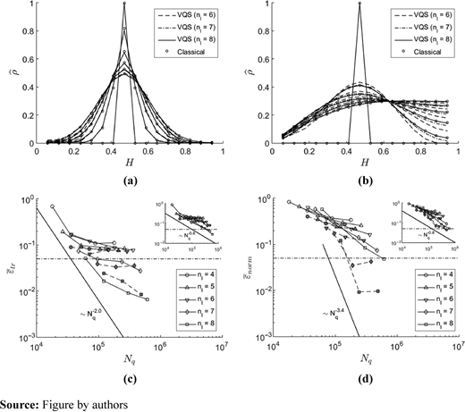
Normalized colloidal probability density profiles without interaction (U = 0) on a 2n = 16 grid using time-step Δτ = 10−4 plotted in increments of (a) 2 × 10⁻³ and (b) 2 × 10⁻² up to T = 10−1. Lines show VQS solutions based on full circular ansatz with six to eight layers, and circles show classical solutions based on the same discretization. Mean (c) trace and (d) norm errors plotted on log scale versus the total number of circuits Nq for run-time up to T = 10−1 (insets show peak values). Data are grouped by the number of ansatz layers, each set using time-step Δτ ∈{10, 5, 2, 1} × 10−4. Closed symbols represent Runge–Kutta solutions using time-step Δτ ∈{10, 5, 2} × 10−4. Horizontal reference line: 0.05
Normalized colloidal probability density profiles without interaction (U = 0) on a 2n = 16 grid using time-step Δτ = 10−4 plotted in increments of (a) 2 × 10⁻³ and (b) 2 × 10⁻² up to T = 10−1. Lines show VQS solutions based on full circular ansatz with six to eight layers, and circles show classical solutions based on the same discretization. Mean (c) trace and (d) norm errors plotted on log scale versus the total number of circuits Nq for run-time up to T = 10−1 (insets show peak values). Data are grouped by the number of ansatz layers, each set using time-step Δτ ∈{10, 5, 2, 1} × 10−4. Closed symbols represent Runge–Kutta solutions using time-step Δτ ∈{10, 5, 2} × 10−4. Horizontal reference line: 0.05
To assess the costs of over-parameterization, we calculate the mean trace error [Figure 4(c)] and norm error [Figure 4(d)] depending on the total number of circuits required Nq for the VQS with a run-time of T = 10−1. Figure 4(c) shows that the mean trace error is insensitive to number of ansatz layers up to six and time-steps up to 5 × 10⁻⁴; it is reduced only with further increase in the number of ansatz layers nl > 6, leading to optimal scaling of . Closed symbols show results using a higher-order Runge–Kutta time-stepping in place of first-order Euler time-stepping [equation (8)]. We see that the cost scaling of the mean trace error is relatively unaffected by higher-order time-stepping, due to the additional circuit count required for four Runge–Kutta iterations per time-step. The peak trace errors follow a weaker scaling of .
Using Euler time-stepping, the mean norm error scales as , regardless of nl [Figure Figure 4(d)]. This cost scaling improves significantly up to using Runge–Kutta time-stepping for circuits with nl > 6. Note, however, that this improvement does not extend to the peak norm errors, whose cost scaling remain as , regardless of time-stepping scheme.
3.1.2 DLVO potential φ(A, Z, κ).
In the presence of colloid–wall interactions, the DLVO potential term φ depends minimally on three parameters, specifically A, Z and κ [equation (22)]. Following the potential-free case (n = 4, H ∈ [0, 1], Δτ = 10−4), we perform VQS including φ using eight ansatz layers in time τ ∈ [0, T].
In the absence of the electric double layer (Z = 0), the DLVO potential φ(A) depends on only the van der Waal’s interaction energy, assumed here to be attractive. Figure 5(a) shows that the DLVO potential φ(H) profiles scaled by the square of the interval ΔH2 for A ∈ {0.05, 0.1, 0.2, 0.5} is only short-ranged in H, so the quantum solution |ρ〉 is insensitive to A. Recall, however, the earlier substitution p(τ) = ρ(τ)e–U/2, such that the actual solution p depends on the longer-ranged interaction energy U(H) [equation (21)], as shown in Figure 5(a, inset). Indeed, space-time plots show that the colloidal probability density p(H, τ) for A = 0.05 up to T = 0.1 is depleted near wall [Figure 5(c)] compared to the potential-free (φ = 0) case [Figure 5(b)]. Increasing A further increases the depletion range [Figure 5(d)].
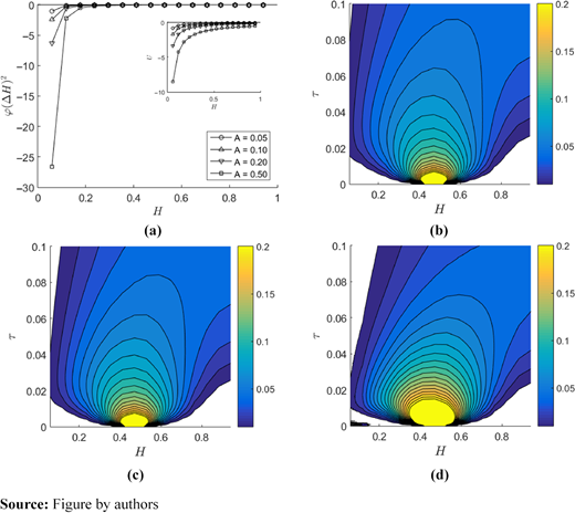
(a) DLVO potential φ(H) profiles scaled by ΔH2 using a full circular ansatz with eight layers for Z = 0 varying A. Inset shows interaction energy U(H). (b–d) Space-time plots of colloidal probability density p(H, τ) ∈ [Δp, 0.2] with contour interval Δp = 0.01. Given Z = 0, (b) φ = 0, (c) A = 0.05 and (d) A = 0.5
(a) DLVO potential φ(H) profiles scaled by ΔH2 using a full circular ansatz with eight layers for Z = 0 varying A. Inset shows interaction energy U(H). (b–d) Space-time plots of colloidal probability density p(H, τ) ∈ [Δp, 0.2] with contour interval Δp = 0.01. Given Z = 0, (b) φ = 0, (c) A = 0.05 and (d) A = 0.5
Otherwise, the DLVO potential φ(A, K, κ) includes the electric double layer interaction energy, assumed here to be repulsive. For A = 0.5, Figure 6(a) shows that the DLVO potential shows short-ranged dependence on Z and κ. However, p depends on the longer-ranged interaction energy U(H) that can be either attractive or repulsive as shown in Figure 6(a, inset). A space-time plot of the colloidal probability density p(H, τ) for {Z, κ} = {10, 10} shows long-ranged influence of the electric double-layer interaction. Parametric analyses of {Z, κ} holding A = 0.5 show that Z depletes p(H, τ) near wall [Figure 6(c)], and a decrease in κ increases the deposition flux and depletion range [Figure 6(d)].
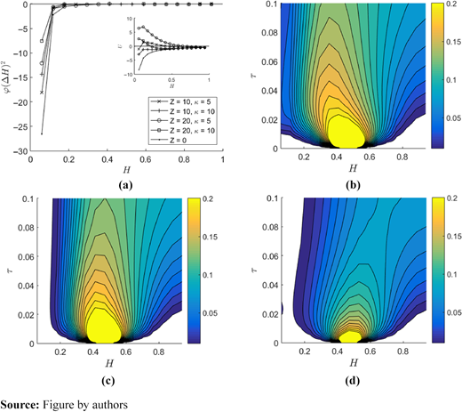
(a) DLVO potential φ(H) profiles scaled by ΔH2 using a full circular ansatz with eight layers with A = 0.5 varying Z and κ. Inset shows interaction energy U(H). (b–d) Space-time plots of colloidal probability density p(H, τ) ∈ [Δp, 0.2] with contour interval Δp = 0.01. Given A = 0.5, {Z, κ} are (b) {10, 10}, (c) {20, 10} and (d) {10, 5}
(a) DLVO potential φ(H) profiles scaled by ΔH2 using a full circular ansatz with eight layers with A = 0.5 varying Z and κ. Inset shows interaction energy U(H). (b–d) Space-time plots of colloidal probability density p(H, τ) ∈ [Δp, 0.2] with contour interval Δp = 0.01. Given A = 0.5, {Z, κ} are (b) {10, 10}, (c) {20, 10} and (d) {10, 5}
3.1.3 Trace and norm errors.
Here, we characterize the effect of DLVO potential on the solution fidelity in time using the trace error εtrace(τ) [equation (15)] and the norm error εnorm(τ) [equation (16)]. Figure 7 shows that εtrace(τ) peaks and decreases during the early diffusion phase [Figure 4(a)], then peaks and decreases again as the normalized probability density approaches a steady-state profile constrained by the imposed asymmetric boundary conditions [Figure 4(b)]. Parametric analyses suggest that the electric double layer coefficient Z has the strongest effect on εtrace(τ) [Figure 7(b)]. In contrast, εnorm(τ) tends towards a steady state regardless of the evolution of probability density. Parametric analyses suggest that εnorm is affected by the local depletion of but insensitive to the magnitudes of A [Figure 7(a)] and Z [Figure 7(b)].
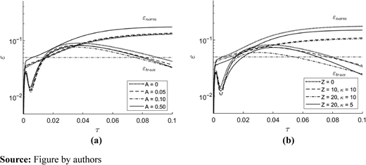
Trace error εtrace and norm error εnorm in time τ for (a) Z = 0, varying A, and (b) A = 0.5, varying Z and κ. Horizontal reference line: 0.05
Trace error εtrace and norm error εnorm in time τ for (a) Z = 0, varying A, and (b) A = 0.5, varying Z and κ. Horizontal reference line: 0.05
Thus concludes our analysis of the potential term in equation (28) in Smoluchowski equation. What usually follows are calculations of survival probability, the probability that the colloidal particle has not reached the wall, the mean first passage time distribution and the mean rate of change of survival probability. Because they do not involve any quantum computation, they are outside the scope of this study. Interested readers are referred to Torres-Díaz et al. (2019).
3.2 Einstein–Smoluchowski equation
The general PDE introduced in equation (1) includes a non-homogeneous source term f, which is not admissible in Smoluchowski’s description of colloidal probability density. To explore the effects of a source term, we switch over to the analogous Einstein–Smoluchowski equation (Cejas et al., 2019; Leong et al., 2023):
which describes the concentration of colloidal particles c(h, t) instead of probability density but is otherwise identical to the Smoluchowski equation [equation (20)]. The difference here is that a continuous concentration source can be imposed as a far-field Dirichlet boundary condition. Rescaling c(H, τ) in space H ∈ [0, 1] and time τ ∈ [0, T], we perform a change of variables c(τ) = ς(τ)e–U/2 as before, and write:
where the operator = X⊗n imposes a unit source in the far field, increasing the required number of quantum circuits by np + 1 [equation (17)] per time-step. The number of additional circuits scales with the number of unitaries required to express .
3.2.1 Initialization.
We seek a parameterized ansatz that encodes a Heaviside step function centred at |2n–1〉:
For a full circular ansatz [Figure 1(d)], this can be encoded on a minimum of two RY parameterized layers by setting the final layer as and the second RY of the preceding layer as , where a reversal in the sign produces a step-down function instead.
3.2.2 Solutions and errors.
We perform VQS on a 2n = 16 grid using time-step Δτ = 10−4 as before, but on a full circular ansatz with five layers, which is already shown to yield high-fidelity solutions [Figure 2(c) and 2(d)]. Figure 8(a) shows how the normalized concentration evolves from the initial step function for the potential-free case (U = 0). In the absence of an electric double layer (Z = 0), strong attractive van der Waal’s energy leads to fast convergence towards a steady-state profile [Figure 8(b)]. Increasing Z shifts the steady-state concentration profile near wall [Figure 8(c)], whereas decreasing κ increases the depletion range [Figure 8(d)]. Both trace and norm errors (Figure 8 insets) decay in time τ towards convergence with εtrace peaking earlier than εnorm.
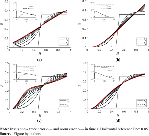
Normalized colloidal concentration profiles on a 2n = 16 grid using time-step Δτ = 10−4 plotted in increments of 10−2 up to T = 10−1 (bold red). Lines show VQS solutions based on the full circular ansatz with five layers. (a) U = 0 and (b) A = 0.05, Z = 0. Given A = 0.05, (c) Z = 20, κ = 10 and (d) Z = 10, κ = 5.
Normalized colloidal concentration profiles on a 2n = 16 grid using time-step Δτ = 10−4 plotted in increments of 10−2 up to T = 10−1 (bold red). Lines show VQS solutions based on the full circular ansatz with five layers. (a) U = 0 and (b) A = 0.05, Z = 0. Given A = 0.05, (c) Z = 20, κ = 10 and (d) Z = 10, κ = 5.
4. Conclusion
Currently, neither VQO nor simulation is capable of realizing an advantage for solving PDEs over classical methods (Anschuetz and Kiani, 2022), but that gap is closing fast (Tosti Balducci et al., 2022). For VQS, a significant progress has been made since the advent of imaginary time evolution (McArdle et al., 2019) notably in the field of quantum finance (Fontanela et al., 2021; Miyamoto and Kubo, 2021; Kubo et al., 2021).
Here, we list a formal approach to solving a 1D evolution PDE [equation (1)]:
{∂tu(t), ∂xxu(t)} terms handled using variational quantum imaginary time evolution.
∂xu(t) term eliminated through substitution methods, such as u(t) = egv(t).
u(t) term included in the Hamiltonian without additional complexity cost.
f(t) term realized by an additional set of complementary circuits, whose complexity depends on .
Superior performance of VQS is contingent on two factors: selection of ansatz and initialization of parameters. Comparing real-amplitude ansätze (Section 2.3), we found that the full circular ansatz significantly outperformed not only linear entangled ansätze but also the popular circularly entangled ansatz but with the final parameterized layer unentangled (Kubo et al., 2021; Alghassi et al., 2022). The advantage in solution fidelity persists over multiple parametric layers, which suggests that unentangled parameterized gates reduce overlap with quantum states that are characteristic of PDE solutions. For an initial state resembling a Dirac delta function (Section 2.4), we found that full circular ansatz can be mapped parametrically to a desired state |x〉, thus reducing subsequent impulse encodings to only a trivial lookup.
As a proof-of-concept, we performed VQS to simulate the transport of colloidal particle to an absorbing wall as described by the Smoluchowski equation (Section 3.1) and found high solution fidelity during the initial spreading of the probability distribution. However, to satisfy the asymmetric boundary conditions, additional parameter layers are required, for example, up to —six to eight layers for a four-qubit problem. Higher-order time-stepping such as Runge–Kutta method can reduce norm errors more effectively than over-parameterization for the same time complexity.
With near-wall DLVO potentials, we found that the van der Waal’s interaction impacts VQS mainly through the potential φ(A) of the Hamiltonian, whereas the electric double layer interaction affects the solution mainly through the factor e–U/2 obtained from change of variables. Simulations of colloidal concentration with unit boundary source in the far field (Section 3.2) require additional circuit evaluations equal to approximately half the number of parameters. Interestingly, this cost is offset by the fact that fewer parameters are required, here, for example, five layers for a four-qubit problem.
Overall, we find VQS an efficient tool for applications in colloidal transport because DLVO potentials do not incur additional costs in terms of quantum complexity. Compared to VQE (Leong et al., 2022), VQS enjoys significant advantages in that it does not require repeated encodings and iterative optimization loops. In terms of scalability, we found that the accuracy of quantum simulation not only depends on the number of qubits but also on the imposed boundary and the initial conditions. As with other gradient-based neural networks, VQS potentially suffers from barren plateau problems, which are exemplified by vanishing gradients on flat energy landscapes (McClean et al., 2018) and exacerbated by quantum circuits with high expressivity (Holmes et al., 2022). Mitigation strategies for barren plateaus remain an active area of research (Patti et al., 2021).
Future work can include extension to 2D model for non-spherical colloids (Torres-Díaz et al., 2019), optimal ansatz architecture (Tang et al., 2021) and initial state preparation (Nakaji et al., 2022; Zoufal et al., 2020).
Notes
For an introduction to quantum computation and Dirac notation, we refer the reader to Nielsen and Chuang (2010).
Not to be confused with the cyclic shift operator in equation (12), also denoted by S.
This work was supported in part by the Agency for Science, Technology and Research (A*STAR) of Singapore (#21709) under Grant No. C210917001. F.Y.L. acknowledges funding support from the RIE2020 Advanced Manufacturing and Engineering (AME) IAF-PP Capsule Surface Affinities (Complete Life-Cycle) grant (Project Ref.: A20G1a0046). D.E.K. acknowledges funding support from the A*STAR Central Research Fund (CRF) Award for Use-Inspired Basic Research (UIBR), as well as the National Research Foundation, Singapore, and A*STAR under the Quantum Engineering Programme (NRF2021-QEP2-02-P03).
The authors acknowledge the use of IBM Quantum services for this work. The views expressed are those of the authors and do not reflect the official policy or position of IBM or the IBM Quantum team.
Author contributions: F.Y.L. designed study; D.E.K. and J.F.K. advised study; F.Y.L. and W.B.E. wrote software code; F.Y.L. and D.E.K. ran simulations and analysed data. All authors wrote and reviewed the manuscript.
Competing interests: The authors declare no competing interests.
Availability of data and materials: The data sets used and/or analysed during the current study are available from the corresponding author on reasonable request.
References
Appendix 1. Quantum circuits to evaluate A and C
The elements of matrix A [equation (6)] and vector C [equation (7)] can be evaluated via sampling the expectation of an observable Z using quantum circuits shown in Figure A1 (Zoufal et al., 2021). The derivative of the trial state with respect to θk is:
such that for a single-qubit rotation gate , the gate derivative is measurable with coefficient fk = –i/2 and a Pauli-Y gate σk = σY inserted in the trial state. Accordingly, the quantum circuit may incur a global phase e–iα, where α = 0 and π/2 for A and C, respectively, which may be rectified through an additional phase gate [2], on the ancilla qubit.
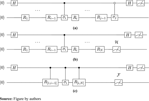
Quantum circuits to evaluate (a) via Hadamard tests, (b) and (c) (Miyamoto and Kubo, 2021) via direct measurements with respect to observables and , respectively (Zoufal et al., 2021)
Quantum circuits to evaluate (a) via Hadamard tests, (b) and (c) (Miyamoto and Kubo, 2021) via direct measurements with respect to observables and , respectively (Zoufal et al., 2021)
We implemented Hadamard tests [Figure 1(a)] in IBM Qiskit using the aer_simulator backend with sampling count of 212 shots per circuit evaluation and direct measurements using statevector_simulator with respect to observables [Figure 1(b)] and [Figure 1(c)]. Note that the latter requires a controlled trial state formed by controlled parameterized unitaries (Miyamoto and Kubo, 2021).
Appendix 2. On the encoding of bit strings using full circular ansatz
In this appendix, we elaborate on the initialization procedure described in Section 2.4 that uses the full circular ansatz of Figure 1(d). Firstly, we note that the ansatz is diagonal in the computational basis and therefore preserves computational basis states. Hence, for the rest of this analysis, it suffices to just consider the action of the ansatz on bit strings. As a function Cn: {0, 1}n → {0, 1}n, the ansatz transforms bit strings as follows in little-endian:
For example, when n = 6, one can check that:
Hence, Cn can be represented as the n × n matrix whose (i, j)-th entry is (Cn)ij = 0 if j > i > 0 or i = j =0, and 1 otherwise. For example, when n = 6, this matrix is given by:
Each layer of entangling CNOT gates (Figure 1) corresponds to an application of the Cn matrix to the input bit string, denoted |x0〉. Successive application of Cn generates a sequence of bit strings , eventually resulting in the initial bit string for some period, p, i.e. , thus forming a periodic sequence or orbit. We illustrate the sequences of bit strings generated by this procedure for the cases of n = 4, 5, 6 in Figure A2. We note that p ≤ 2n – 1, and in the cases where p < 2n – 1, there are disjoint orbits corresponding to the different irreducible representations of the full circular ansatz group. The trivial one-dimensional irrep corresponds to the all-zeroes bit string |00…0〉 set by θ = 0. For n = 4, the strings form two distinct orbits, whereas, for n = 5 and 6, the strings form four distinct orbits (see Figure A2). For n = 4 and 6, all the orbits, save the singleton orbit comprising the all-zeroes bit string, contains at least one string of positive Hamming weight, and hence all 2n – 1 states of positive Hamming weight are reachable from the strings of unit Hamming weight. This is not the case for n = 5, where all the strings of unit Hamming weight are in the same orbit (namely, the orbit of size 21); hence, only these 21 strings out of the 25 – 1 = 31 strings of positive Hamming weight are reachable from the strings of unit Hamming weight.
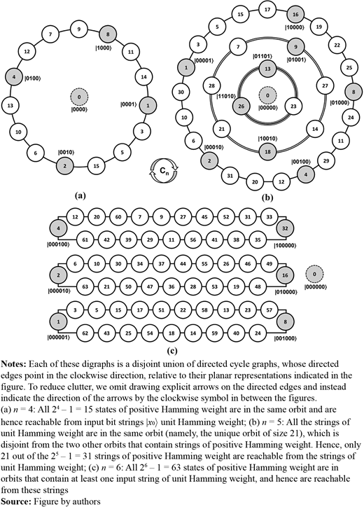
Directed graphs (digraphs) depicting the disjoint orbits arising from applying the Cn matrix to the computational basis states
Directed graphs (digraphs) depicting the disjoint orbits arising from applying the Cn matrix to the computational basis states
