


The Orange River is one of the largest river basins in southern Africa. Since it plays a crucial role in the region's ecology and economy, it is important to estimate future developments in its hydrology. A necessary means to this end are climate projections. This paper seeks to address this issue.
In this work the authors present projections obtained by two complementary methods; they use a Statistical Analogue Re‐sampling Scheme (STARS) and a dynamical regional climate model (CCLM – COSMO in Climate Mode). In order to determine the viability of these methods, the authors perform cross‐validations for the years 1976‐2000.
CCLM shows good performance regarding the 2 m temperature but the reproduction of precipitation is rather poor. STARS, on the other hand, produces very good results for both variables. The climate projections of both models show a considerable temperature increase for the future (2036‐2060, SRES A1B scenario), especially in the inland of the simulation area. However, while CCLM projects a general decrease in precipitation, STARS indicates a strong precipitation decrease in the already dry western part of the region and a moderate decrease resp. no change in the east during the rain season.
For the first time the statistical approach used gridded data as its input. Therefore, it was possible to apply complementary methods in order to generate the climate projections and to compare them.
1 Introduction
In this work the authors present two climate projections for southern Africa. These projections were made in the context of the Transboundary Water Management project in the Southern African Development Community (SADC, www.sadc.int). A subproject of this concerned the Orange River basin, and was carried out under the supervision of the Orange‐Senqu River Commission (ORASECOM, www.orasecom.org). Impact studies are a widely used and crucial tool to anticipate possible impact risks, see, e.g. de Wit and Stankiewicz (2006), Thomas et al. (2007) and Lobell et al. (2008).
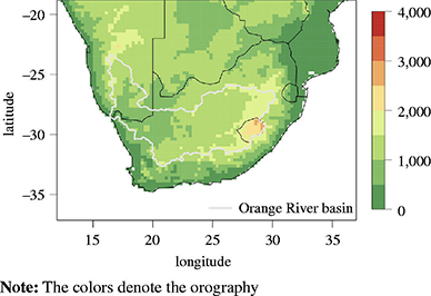
The Orange River basin is located in southern Africa (Figure 1). It is the longest river in the region with a length of 2,200 km. Its basin covers an area of almost 1,000,000 km2 and affects the livelihood of the four nations South Africa, Namibia, Botswana and Lesotho. Its spring is in the Drakensberg mountains in Lesotho, from where it flows westward to the Atlantic Ocean, passing through vastly different areas such as mountains, dry grasslands and finally arid landscapes. There is a strong rainfall gradient from east to west: the mountain regions in Lesotho have an annual precipitation of up to 2,000 mm, whereas the region around the mouth of the river hardly gets 50 mm per annum. The temperature gradient in the interior of southern Africa is strong as well. The daily mean temperatures range from approximately 10°C in the Lesotho Highlands to more than 22°C at the river mouth. This contrast is even more pronounced when looking at the extreme temperatures. The desert regions at the lower Orange River can reach very high temperatures of up to 50°C while frost days are common in the mountain region.
The natural water discharge is highly variable and dependent on climate. The Orange River plays an important role in the region's ecology and economy. The large Gariep and Vanderkloof dams provide hydro‐electric power and water for irrigation, mining and industry. Water is even transferred through various river/tunnel systems beyond the basin boundaries. The water of the Orange River is in such demand that these transfer schemes are still being expanded (e.g. the Lesotho Highlands Water Project). Thus, it is important to investigate the possible hydrological developments in this region, which in turn depend on the future climate. In this work, the authors focus only on the climate projections, though.
The authors use two complimentary approaches for climate modeling, one statistical and one dynamical (Murphy, 1999; Xu, 1999). Typically, the output of general circulation models (GCMs) is used to drive regional climate projections. Statistical modeling uses past observations and reassembles them according to the trend prescribed by the GCM. In the dynamical approach a regional climate model (RCM) like COSMO in CLimate Mode (CCLM) (Böhm et al., 2006) is nested into the GCMs. Similarly to the GCMs, the simulations of RCMs are based on physical processes, but they take place on a smaller temporal and spatial scale. Thus, RCMs allow for an analysis of the interactions between different climate processes and their effects. This feature is very important for climate projections of the distant future, when the future climate and the present climate will most likely differ substantially (Solomon et al., 2007).
The high climatological variability in southern Africa is a challenge for every RCM because most models include physical parameterizations that are mainly tested and optimized for one specific climate regime; this is particularly true for dynamical models. Although current RCMs are able to reproduce the main climatic features in different regions of the world, they tend to perform much better in their “home region” (Rockel and Geyer, 2008). STatistical Analogue Re‐sampling Scheme (STARS) was developed and elaborately tested in Germany (Orlowsky et al., 2008). However, as STARS reproduces only spatial patterns which have been observed before, the simulated spatial variability is expected to be consistent with the observations. This feature has already been successfully demonstrated in Orlowsky et al. (2010) for station data in China. In this paper, STARS is applied for the first time with gridded data to provide spatial fields instead of single station time series. Hence, the authors are able to analyze the performance of STARS in this climatically interesting and varying region. Furthermore, they can compare the results to those simulated by CCLM.
This paper is structured as follows. Section 2 introduces the main principle of STARS and CCLM, while the data and the experiment set‐up are described in Sections 3 and 4. Section 5 analyzes the cross‐validation experiment which demonstrates the applicability of STARS and CCLM to southern Africa. The results of the climate projections for the years 2011‐2060 are illustrated in Section 6. Finally, Section 7 draws some conclusions.
2 Methods and models
2.1 Statistical downscaling and STARS
Statistical downscaling refers to either of three methods: regression models, analogue methods (Wilby et al., 1998; Zorita and von Storch, 1999) and stochastic weather generators (Wilks, 1999). Regression models analyze statistically derived relations between the output of GCMs and regional weather. Analogue methods look for the circulation pattern in the past which is most similar to a certain pattern simulated (by a GCM) in the future and assign the associated regional weather to the future date. The obtained combinations of variables are physically consistent for both methods. However, their projections depend on the performance of one or several GCMs, which might be poor for certain regions and variables (Giorgi and Francisco, 2000; van Ulden and van Oldenborgh, 2006). Weather generators are less dependent on GCMs. They generate time series of single climate variables that are conditioned by prescribed general time series statistics. However, the results are often physically inconsistent because they usually generate time series for different variables individually. The applications of statistical downscaling are limited to near future projections, or more generally to simulations of a similar climate, as these implementations do not overstress the stationary assumption that is characteristic for statistical approaches.
The STARS used in this study combines the advantages of the analogue methods (physical consistency between different variables) and the weather generators (independence of GCM output). It generates ensembles of daily time series that optimally fit a linear temperature trend (Orlowsky et al., 2008). This temperature trend is the only constraint for the resampling. It can be derived from GCM output, but it is also possible to prescribe different linear temperature trends to estimate the response of the climate. In this study the authors compute climate projections using four different prescribed temperature trends.
The model STARS has been developed in different stages over a long time period (Werner and Gerstengarbe, 1997; Orlowsky et al., 2008). The most recent model version is described below. However, one should keep in mind that the model is under continuous development. The following description of the methodology is short as the authors mainly focus on the impact analysis. However, it is based on the paper by Orlowsky et al. (2008), where more details can be found.
STARS presupposes that weather situations which have been observed in the past are likely to recur in the same or very similar way during the simulation period. Hence, simulated series are constructed by resampling from segments of observation series, consisting of daily observations. The obvious advantage of such a resampling method is that the resulting series consist of observations of different meteorological parameters of the same day, which are therefore physically consistent, as they are former real‐world observations. This applies analogously to the spatial fields of the meteorological variables. Note that STARS, unlike weather generators, rearranges only one meteorological variable according to the given trend. The other variables are taken from the same day as the “forcing” variable. Therefore, no multiple regression analysis is needed at the end of the computations.
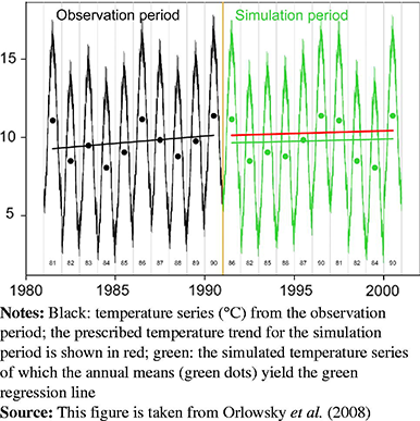
The resampling is constrained by a very simple forcing that can be easily checked for plausibility: the simulated annual means of a chosen climate variable have to correspond to the parameters of a linear regression line, i.e. mean and slope. The climate variable is to be chosen such that it captures the essential climate variability of the region of interest. Typically, the 2 m temperature is chosen because the increase of temperature is one of the most robust climate signals for most regions of the world.
Figure 2 shows the model principle. The model input consists of a time series of observations and a regression line (in case of temperature: the average temperature and the long‐term linear temperature increase) for the simulation period. A simulated time series is constructed by rearranging the observations using the Monte Carlo method in such a way that the annual means follow the prescribed regression line as precisely as possible. This algorithm, however, does not completely determine the simulated series. In addition a set of heuristic rules for the resampling is defined, which ensures that the resulting series complies not only with the prescribed trend but are also realistic with respect to characteristics like annual cycles, variability, persistence, etc.
The above model description assumes simulations with only one station, though the approach is the same in case of multi‐station data. The comparison between the achieved and the prescribed trend is done collectively, so that the order of the rearrangement is the same at all stations. The results are spatial fields that have been already observed in the past. To reduce complexity while simultaneously maintaining the spatial patterns, the model area is divided in climatically similar subregions. This is done by a hierarchical spatial cluster analysis based on temperature and precipitation. A representative station (the center of mass of the cluster class) then represents each subregion. It is possible to work with spatially resolved trends if the trend is derived from GCM output, so that different spatial developments are accounted for. If the trend is assigned for the entire simulation area (as in this study), the model rescales the value for each representative station, assuming constant ratios between the observed trends and the simulated trends at these stations.
In contrast to dynamical RCMs, STARS is able to generate large ensembles of climate projections using little computational power. In addition, the availability of station data as well as the resolution of reanalysis data has improved considerably so that the application of STARS becomes more feasible for different regions of the world. Although statistical models have consistently outperformed dynamical RCMs in validations, dynamical RCMs have an important advantage over the statistical approach: they are based on physics and consider physical processes, so that process studies can be performed with RCMs only. Besides, STARS is not able to generate new absolute extremes as the model only rearranges already observed values. Usually, a resampling with STARS can only be done at points where a meteorological station is located; however by the novel approach employed in this paper, this limitation has been overcome.
2.2 Dynamical downscaling and CCLM
Besides statistical downscaling the authors use dynamical downscaling as a complementary approach. “Dynamical” means that, unlike STARS, differential equations that describe physical processes are solved. For instance, the atmosphere is considered to be an ideal gas, and its movements are modeled according to Newtonian laws of motion. Similarly, water and energy transport in the soil are modeled according to the Richards equation resp. the heat equation.
Like most dynamical RCMs, CCLM originates from a numerical weather prediction (NWP) model. It is an offspring of Lokalmodell (LM), the predecessor of Deutscher Wetterdienst's current and operational NWP model COSMO. In the early 2000s, features necessary for climate simulations were implemented on top of LM/COSMO, and in 2005 the model was named CCLM. In 2007/2008 both development branches, COSMO and CCLM, were merged back together, and CCLM became the official dynamical RCM of the German climate modeling community. Currently, CCLM is used by a growing community of more than 40 institutions in Asia, Europe and America.
CCLM was originally developed for applications in mid‐latitude areas, such as Europe, but has been increasingly used in other regions of the world. For instance it was run for Asia, South America, Africa, etc. In fact, results from a previous run over Africa are used here (see Section 4.2). Generally, CCLM covers an area at the mesoscale, i.e. areas between 100 and 10,000,000 km2. The resolution is typically in the range from a few kilometers up to, approximately, 50 km. The time frame to be simulated varies from several years up to centuries; usually simulations are run for several decades.
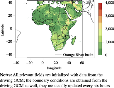
CCLM, like other dynamical RCMs, requires data from a GCM to initialize the region to be simulated, and to drive it at the boundaries. The setup is shown in Figure 3, where the typical size of simulation areas can be seen as well. As stated, values within the area in question, such as sea surface temperature, air temperatures, soil water content, etc. are initialized with data from a GCM. Then, the equations from the physical description of the air, soil, and so forth are numerically solved. At certain intervals, in our case every six hours, boundary data from a GCM is fed into the model.
The fact that RCMs are based on physical principles/models allows researchers to qualitatively and quantitatively investigate the nonlinear processes inherent to climate science. Furthermore, hypothetical scenarios, such as land use/land cover changes, can be examined. Dynamical models provide a lot of different variables at every point in space and time, unlike statistical models which are confined to the variables and positions of their input data. Potentially, a dynamical RCM can incorporate many submodels, such as urban models, lake models, etc. However, a dynamical model can never escape its driving GCM, so any GCM bias is bound to show up in the RCM simulation as well. Due to the nesting procedure, there is no feedback to the driving GCM, so energy and momentum conservation is broken. Running a dynamical RCM is computationally rather expensive (depending on the chosen resolution/area), especially when compared to statistical downscaling. With STARS 1,000 realizations can be computed in one day, while CCLM requires approximately three months for one realization. Hence, only few simulation runs can be computed for a simulation area, making it hard to estimate the model uncertainty for climate projections.
3 Data
STARS rearranges observational station data to generate ensembles of future climate projections. In this study WATCH data (Weedon et al., 2011) from 1951 to 2000 is used. It is available on a regular grid with a resolution of 0.5°×0.5°. The daily time series of the following variables are used in the presented work: mean, minimum and maximum 2 m temperature, precipitation, relative humidity, short wave radiation, wind and air pressure. The long term averages of the 2 m temperature and of the precipitation are shown in Figures 4 and 5.
As stated above, climate projections from STARS are constrained by a linear temperature trend. In this work the authors use four different temperature trends. Thus, the projections have been carried out according to four different scenarios. Note that the temperature trend is not derived from a GCM in this study.
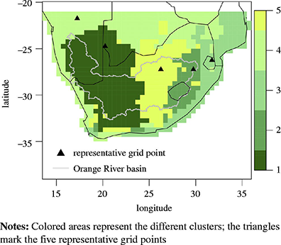
The simulations are carried out for the Orange River basin and its surroundings. They cover 904 grid points with a resolution of 0.5°×0.5°, ranging from 21°S to 35°S and from 14°E to 36°E. The simulation area is split into five climatological subregions based on a hierarchical cluster analysis, as shown in Figure 6.
4 Experiment set‐up
4.1 STARS
To test the applicability of STARS to southern Africa, a cross‐validation experiment is carried out. However, a positive cross‐validation experiment is a necessary but not a sufficient condition for the calculation of climate projections. The input data is split into two periods of 25 years: the observation period 1951‐1975, and the validation period 1976‐2000. The climate of the validation period is simulated using the first 25 years and the observed trend of the annual mean temperature. This trend is derived from the data by a regression analysis of the annual mean temperature series at the five representative grid points. It ranges from 0.2°C to 1.4°C. The model reproduces the given trend with a user‐defined tolerance. For the cross‐validation this tolerance is chosen to be between 0.1°C and 0.2°C. The performance of STARS is evaluated comparing the simulated climatology with the observed one in the validation period. An ensemble of 1,000 simulations is generated to quantify the model uncertainties.
Two of the representative grid points do not fulfill the “internal variability conservation” criterion (Orlowsky et al., 2010). This criterion says that only if the temperature anomalies of the input data and the simulated series can be seen as originating from the same distribution, the variability of the input data is large enough to generate series with a given temperature trend without a statistically visible reduction of variability. In various tests Orlowsky found that this criterion is only fulfilled when the warming in the simulated period continues with the same strength as in the training period. In case of the two grid points mentioned above, the annual mean temperature shows only a weak trend or even a temperature decrease during the first time period, while the annual means for the same grid points increase strongly during the validation period. Therefore, the successful cross‐validation despite this demanding setting gives strong evidence of the robustness of the projections.
After the cross‐validation experiment future climate projections are computed for the time period 2011‐2060. To avoid the dependency on GCMs and associated uncertainties, the projections are carried out using four different scenarios: no temperature trend, a trend of 0.5°C, a trend of 1°C and a trend of 1.5°C for the simulated time period. Note that the SRES A1B scenario (Nakicenovic et al., 2000) results in a temperature trend of 1.6°C for the simulation area and the simulation time period. This means that the projections done by CCLM are to be compared to the 1.5°C scenario computed by STARS.
The simulations for each scenario contain 1,000 ensemble members. From this large sample the authors randomly draw 100 simulations without replacement to reduce the amount of data. Furthermore, only the ensemble median is chosen for a detailed analysis of the climate projections in this work.
4.2 REACCT
The authors use CCLM runs that were originally carried out for the Resilient Agro‐landscapes to Climate Change in Tanzania project (REACCT, www.reacctanzania.com). Since Africa is centered around the equator, there was no need for a rotated coordinate system. The simulation area stretches from 42.25°N to 45.75°S resp. from 24.75°W to 60.25°E. The resolution is 0.5°×0.5° which amounts to 56 km×56 km.
For the validation the authors simulated the years 1976‐2000. The simulations are driven by an ECHAM5 (Roeckner et al., 2006) run that was in turn driven by twentieth‐century (C20) greenhouse gas (GHG) concentrations. The projection covers the years from 2001 to 2100. It is driven by ECHAM5 results as well, which are based on the SRES A1B (Nakicenovic et al., 2000) scenario.
5 Validation
5.1 Validation STARS
The comparison between the observed and the simulated climate in the validation period (1976‐2000) leads to the following results:
The agreement between the climatological means is very good for all statistics and variables analyzed (not all are shown here).
The simulated spatial patterns of all variables are very similar to the observations.
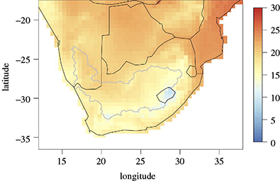
The long time average of the mean, maximum and minimum temperature shows a slight overestimation of up to 0.4°C. The strongest overestimation occurs in the interior of the simulation area (Figure 7). However, the temperature bias was statistically tested using the Wilcoxon‐Mann‐Whitney test (Hollander and Wolfe, 1999) with a significance level of 5 percent: there is no significant difference between simulated and observed temperature for the whole simulation area.
In terms of precipitation the results are very good. Actually, precipitation is rather difficult to simulate, thus it is a challenge that many regional models cannot cope with (Kotlarski et al., 2005). The long term average of the precipitation (Figure 8) indicates that STARS overestimates precipitation in general by approximately 10 percent or even less. The overestimation reaches values of up to 50 percent in the arid areas of Namibia. Despite the low bias, the difference between simulations and observations is significant (Wilcoxon‐Mann‐Whitney test with a significance level of 5 percent) for most parts of the simulation area, except Lesotho and Swaziland and surroundings. However, the mean annual cycle of the precipitation at the representative grid points shows that the model mostly underestimates precipitation in the rainy season (not shown). The precipitation in the rainy season is very well reproduced only for the representative grid point of the mountainous cluster, where Lesotho is located. Furthermore, the extreme rainfall (90th percentile of the precipitation and duration of dry days) at the representative grid points is reproduced well.
Figure 9 shows the spatial similarities for precipitation between the different realizations and the observations for the validation time period using a Taylor diagram (Taylor, 2001). This kind of illustration shows not only the spatial correlation between the simulations and observations, but also the similarity of spatial variability. It includes correlations, variability values (i.e. standard deviations) and the centered root‐mean‐square differences and is useful for comparing multiple data sets to a reference data set. As can be seen, the similarity between the different ensemble members (STARS) and the observations is very high and the standard deviations of the simulations are very close to the observations. CCLM, on the other hand, shows a comparatively lower correlation and standard deviation, and a larger RMS difference.
Figures 10 and 11 show the results for the mean annual cycles of mean, maximum and minimum temperature, precipitation, humidity, air pressure, radiation and wind. The annual cycle averaged over the validation period and the simulation area for each variable is illustrated in the upper parts of the plots. The observations are shown in red, while the spread of the simulations is shown in gray, including the ensemble mean in black. The inter‐quartile range and the range between the 10th and the 90th percentile are also illustrated in gray. The two figures show that the spread of the ensemble is narrow and always contains the observed values.
5.2 Validation CCLM
The authors validate CCLM's performance for the years 1976‐2000. The variables investigated are the 2 m temperature and precipitation. The validation run is driven by the ECHAM5 C20 run that was originally carried out for the IPCC AR4 (Solomon et al., 2007). As in the case of STARS, the authors validate against the WATCH data set.
Figure 4 shows the observed annual average temperature in the region according to the WATCH data set. The CCLM bias is plotted in Figure 12. As one can see, the performance of CCLM varies considerably throughout the region. Some areas, in particular deserts like the Kalahari or the Namib, are simulated with statistically significant excessive temperatures (Wilcoxon‐Mann‐Whitney test, α=0.05 (Hollander and Wolfe, 1999)). In the Namib Desert the annual 2 m temperature bias amounts to as much as 6°C. Other areas, especially the mountainous areas around Lesotho, the Drakensberg mountains and the eastern coast show an underestimation of temperature. For the remaining areas, such as the Orange River basin, the temperature is simulated reasonably well.
Similarly to the case of the 2 m temperature, observations (Figure 5) and the corresponding bias (Figure 13) for the total annual precipitation are shown. In Figure 13 one can see that the CCLM performance in reproducing the southern African precipitation is rather poor. Throughout most of the region precipitation is too high, the overestimation for large parts of South Africa, Botswana and Namibia amounts to 100 percent. On the Namibian coast the relative overestimation is even higher, but here precipitation values are very low in the first place. In southern Mozambique, on the other hand, CCLM shows a rather large negative bias, reaching occasionally values of −50 percent. The large bias in Lesotho is particularly unfortunate, since most runoff for the Orange River is generated in the Lesotho highlands. This renders CCLM results unsuitable for hydrological impact modeling in this area. These deviations exemplify the need to fine‐tune CCLM better to the study area.
6 Climate projections
6.1 Climate projections with STARS
The 0°C trend scenario of the climate projections is a control run. As expected, the comparison of the corresponding simulations and the observations provide very good results, underlining the good performance of STARS in southern Africa (not shown).
In Figures 10 and 11 the differences between the last 25 years of the future projections (2036‐2060) and the observations of the validation time period for the mean annual cycles are shown below the mean annual cycles for the validation period (1976‐2000). For the 1.5°C trend scenario the ensemble spread is again shown in gray (the same applies to the inter‐quartile range and the range between the 10th and the 90th percentile, the solid black line indicates the ensemble mean). Only the ensemble mean is shown for the other scenarios.
The differences between the future time period and the validation time period for the mean, maximum and minimum temperature show an increase for the future. But while the mean and maximum temperature rise especially in March and November, the increase of the minimum temperature has its maximum from March to November, the period of lowest temperatures in southern Africa. The temperature increase coincides with an increase in radiation that is most profound in March, but also in austral spring.
The results for precipitation indicate a strong decrease of over 25 percent in austral summer, which is the rain period in southern Africa. However, there is a slight precipitation increase in autumn and spring. A similar pattern can be found for the humidity, but in this case there is no pronounced increase in May and September. The changes in wind and air pressure are very small or nonexistent.
Figures 14 and 15 show the difference between the future projections and the observations for the long term averages of temperature and precipitation. The change between projections and observations in the past is again statistically tested using a Wilcoxon‐Mann‐Whitney test with a significance level of 5 percent. To compare the future projections with the observations for the validation time period, the authors consider only the last 25 years of the simulations (2036‐2060). Of course, the strongest difference can be found in the 1.5°C scenario. However, the spatial patterns described below hold just as well for the 0.5°C and the 1°C scenario, except the changes are not as strong as in the 1.5°C scenario (not shown).
Figure 14 shows a strong, significant temperature increase for the interior of southern Africa (especially Namibia) with up to 2°C for the austral summer. However, the temperature increase is very moderate and not significant along the coastlines of Mozambique and South Africa and at the river mouth (below 0.5°C). In austral winter, the strongest temperature increase also occurs in the inland regions of the simulation area. But this increase is less than in summer with values up to 1.5°C. Due to a more uniform warming, the coastal areas get relatively warmer than in summer.
The inland warming coincides with a general decrease of precipitation in the center of the simulation area. As shown in Figure 15 the decrease of precipitation is strongest in summer (DJF) during the rain period. This is also the time when the change in precipitation is predominantly significant. In the arid areas (central South Africa, Namibia and Botswana) the monthly mean of the summer precipitation decreases by over 50 percent, whereas the summer precipitation increases by up to 40 percent in southern Mozambique. In this context it is important to look at Lesotho, where the predominant water volume of the Orange River originates. There, the summer precipitation decreases significantly by up to 30 percent, which would result in a severe change for the Orange River. The right part of Figure 15 shows that the changes are small and mostly not significant for the austral spring and fall. However, there is a precipitation increase in winter (JJA), when the precipitation typically reaches its lowest values. Especially Lesotho, eastern South Africa and Swaziland expect a (partly significant) increase of up to 40 percent. The amounts of precipitation in the north‐western parts of the simulation area are very low in this time of year, so that the values of the relative change are neglected.
6.2 Climate projections with CCLM
Figures 16 through 19 show the CCLM projection results for the individual seasons. More precisely, the difference between the average 2 m temperature during the projection period 2036‐2060 and the reference period 1976‐2000 is depicted. All CCLM projection changes are measured against the CCLM C20 simulation, instead of the WATCH data, since this might even out model biases. According to CCLM, the increase is unevenly distributed across the seasons. In summer (DJF) and fall (MAM) the temperature is projected to increase by more than 2.5°C in the northern Orange basin, and in Namibia in general. The largest increase is predicted for the Kalahari in summer, and amounts to 3°C. In fall and winter, an increase in the 2 m temperature is projected as well; however the increases are not as severe as in summer and fall. They range between 1°C and 2°C. Overall, the temperature change projected by the A1B scenario amounts to about 1.6°C, but compared to STARS for the 1.5°C scenarios, CCLM sees more drastic temperature increases in some areas. For instance, while STARS projects an increase of about 2°C for the Kalahari in summer, CCLM sees an increase of up to 3.5°C there.
For precipitation the authors show only the result for the annual average projection, because the validation turned out to be rather poor. The projection changes are shown in Figure 20. Generally, CCLM projects a decrease in precipitation, while STARS projects a decrease in the center of the simulation area and no change or increases in the east (not shown). In the areas where CCLM projects the largest decreases, the biases were largest, though, particularly in Namibia.
7 Conclusions
The STARS and CCLM were used to generate future climate projections for southern Africa. A validation experiment affirmed the applicability of STARS to southern Africa, yielding excellent results despite the demanding simulation area with high climatological variability. CCLM, on the other hand, performed reasonably well in the reproduction of the 2 m temperature, but for precipitation the validation results turned out to be poor.
With STARS the authors generated ensembles of future climate projections based on daily gridded data for the time period from 1951 to 2000 for four different scenarios, given as a mean temperature trend over the time period from 2011 to 2060. In these projections the mean, maximum and minimum temperature showed a significant increase, especially in the interior of southern Africa. Such an increase is also projected by CCLM, but the spatial and temporal patterns in the projected temperature increase differ from STARS. While STARS projects local increases of up to 2°C, CCLM sees seasonal increases of up to 3.5°C.
The area‐averaged precipitation, as simulated by STARS, decreases by over 25 percent in the rainy season (DJF). However, there is a slight increase in autumn and spring. The long term average of the spatial distribution (STARS) shows that the precipitation decreases mainly in the inland regions of southern Africa. This decrease is especially profound in austral summer with values of up to 50 percent. In Lesotho, where the Orange River has its spring, and where its main runoff is generated, the precipitation decreases significantly by approximately 30 percent in summer. In contrast, the winter precipitation increases significantly by approximately 40 percent in Swaziland and the northeastern part of the simulation area. CCLM results with respect to precipitation seem not to be reliable.
Due to the projected precipitation changes, the authors suggest that the effects on the Orange River catchment and associated consequences for the ecology and economy should be analyzed using a hydrological model.
As a consequence of its design, STARS is not able to simulate a climate that is essentially different from the present climate (unlike CCLM), since it is based on the assumption that statistical properties of the different variables are the same in the observation and the future time period. This is why the climate projections in this study cover only the years from 2011 to 2060.
Due to very good results in the past (Orlowsky et al., 2008, 2010; Orlowsky and Fraedrich, 2009), STARS is more and more accepted as a stand‐alone climate modeling approach. This study likewise emphasizes the good performance of STARS using gridded data as model input for the first time.
The observed annual average of the 2 m temperature (°C) from 1976 to 2000 (WATCH)
The observed annual average of the 2 m temperature (°C) from 1976 to 2000 (WATCH)
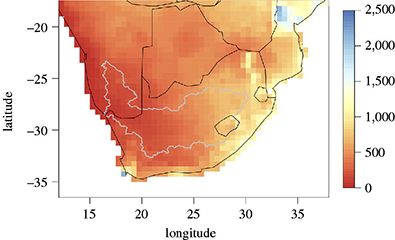
The observed annual average of total precipitation (mm) from 1976 to 2000 (WATCH)
The observed annual average of total precipitation (mm) from 1976 to 2000 (WATCH)
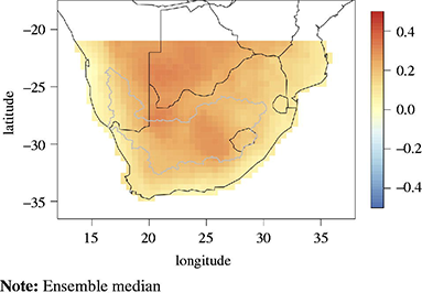
The bias in the long term average of the 2 m temperature (°C) for the validation time period 1976‐2000 as simulated by STARS
The bias in the long term average of the 2 m temperature (°C) for the validation time period 1976‐2000 as simulated by STARS
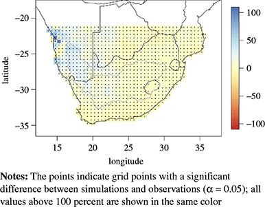
The bias in the long term average of the precipitation (%) for the validation time period 1976‐2000 as simulated by STARS (ensemble median)
The bias in the long term average of the precipitation (%) for the validation time period 1976‐2000 as simulated by STARS (ensemble median)
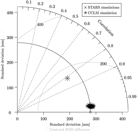
Similarities of the spatial precipitation pattern between the observations and the simulations for STARS and CCLM for the validation time period 1976‐2000
Similarities of the spatial precipitation pattern between the observations and the simulations for STARS and CCLM for the validation time period 1976‐2000
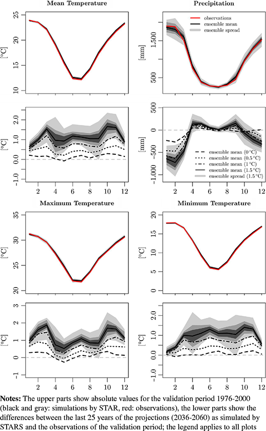
Mean annual cycle of temperature (mean, maximum and minimum) and precipitation
Mean annual cycle of temperature (mean, maximum and minimum) and precipitation
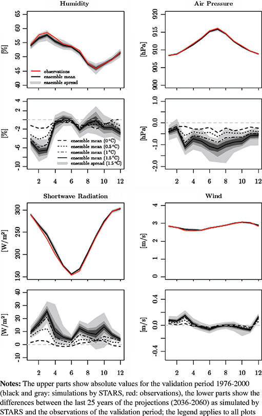
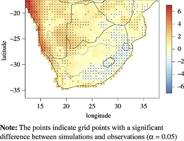
The bias in the annual average 2 m temperature (°C) from 1976 to 2000 as simulated by CCLM
The bias in the annual average 2 m temperature (°C) from 1976 to 2000 as simulated by CCLM
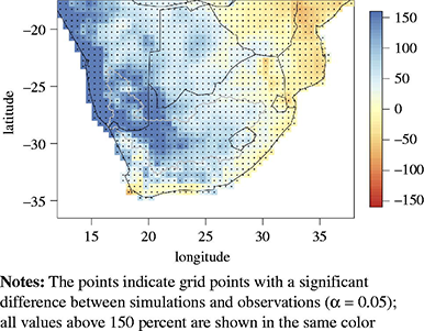
The relative bias in the annual average of total precipitation (%) from 1976 to 2000 as simulated by CCLM
The relative bias in the annual average of total precipitation (%) from 1976 to 2000 as simulated by CCLM
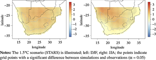
The projected change in the mean temperature (2036‐2060 compared to 1976‐2001) is shown in (°C)
The projected change in the mean temperature (2036‐2060 compared to 1976‐2001) is shown in (°C)
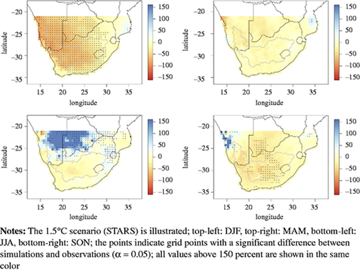
The projected change in the precipitation (2036‐2060 compared to 1976‐2001) is shown in (%)
The projected change in the precipitation (2036‐2060 compared to 1976‐2001) is shown in (%)
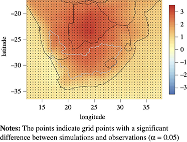
The projected change in the DJF 2 m temperature from 2036 to 2060 when compared to 1976‐2000
The projected change in the DJF 2 m temperature from 2036 to 2060 when compared to 1976‐2000
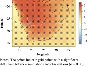
The CCLM‐projected change in the MAM 2 m temperature from 2036 to 2060 when compared to 1976‐2000
The CCLM‐projected change in the MAM 2 m temperature from 2036 to 2060 when compared to 1976‐2000
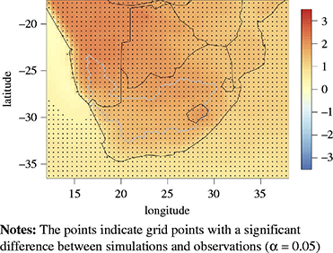
The CCLM‐projected change in the JJA 2 m temperature from 2036 to 2060 when compared to 1976‐2000
The CCLM‐projected change in the JJA 2 m temperature from 2036 to 2060 when compared to 1976‐2000
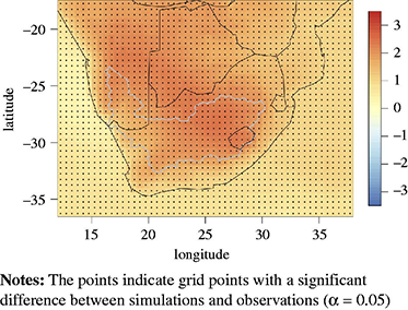
The projected change in the SON 2 m temperature from 2036 to 2060 when compared to 1976‐2000
The projected change in the SON 2 m temperature from 2036 to 2060 when compared to 1976‐2000
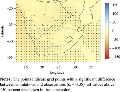
The projected change in the annual average precipitation from 2036 to 2060 when compared to 1976‐2000
The projected change in the annual average precipitation from 2036 to 2060 when compared to 1976‐2000
This work was supported by the authors' partners GIZ, ORASECOM and WRP. The authors are grateful for their support and pleasant collaboration. The CCLM climate simulations were provided by Matthias Büchner (PIK).
References
About the authors
Julia Lutz studied physics and meteorology and graduated with a diploma in meteorology from Rheinische Friedrich‐Wilhelms Universität in Bonn. Currently she pursues her PhD at PIK. She works mainly on statistical downscaling (STARS). Her research focus is on Africa and Europe. Julia Lutz is the corresponding author and can be contacted at: lutz@pik‐potsdam.de
Dr Jan Volkholz studied physics at University of Texas in Austin and Humboldt University Berlin where he acquired his PhD in physics. Currently he works at PIK in Potsdam. His research interests are regional downscaling (CCLM) and climate projections with a particular focus on hydrology.
Professor Dr Friedrich‐Wilhelm Gerstengarbe studied meteorology at Humboldt University Berlin. He obtained his PhD in 1984 and his State doctorate in 1997. Since 2004 he has been Professor for Systematic Climatology at the Humboldt University. Furthermore, he is Assistant Director of PIK and co‐chair of the research domain “Climate impacts and vulnerabilities”. Research fields: Definition of problem‐solving answers to questions related to the influence of climate on environment and society using dynamical and statistical model approaches, global and regional climate analysis, investigation of extreme meteorological and climatological events, development of statistically based climate scenario models.

