

Climate change will have a significant impact on China’s potential agricultural production and change the distribution of the population in various regions of China, thus producing population migration. This paper aims to analyze China’s population migration in response to climate change and its socio-economic impact.
In this paper, the Potential Agriculture Production Index is introduced as an analytical tool with which to estimate the scale of the population migration induced by climate change. Also, this paper constructs a multi-regional computable general equilibrium (CGE) model and analyzes the effect of change in the population distribution pattern on regional economies, regional disparity and resident welfare.
The key finding of this paper is that, as a result of changes in potential agricultural production induced by climate change, the Circum-Bohai-Sea region, the industrialized region and the industrializing region, which are the main destination regions of the migrating population, will face a severe labor shortage. In response to population migration, the economic growth rate of the immigrating population regions has accelerated. Correspondingly, the economic growth rate of the emigrating population regions has decreased. In addition, the larger the scale of population migration is, the larger the economic impact is. Migration increases inner-regional disparity and decreases inter-regional disparity. However, overall regional disparity is only somewhat decreased.
This paper introduces a Potential Agriculture Production Index to estimate the scale of the population migration and introduce a multi-regional CGE model to analyze the correlated social-economic impacts.
1. Introduction
The implications of environmental change for migration are little understood. Migration as a response to climate change could be seen as a failure of in situ adaptation methods, or migration could be alternatively perceived as a rational component of creative adaptation to environmental risk (Bardsley and Hugo, 2010). Climatic variability and change are known to influence human migration patterns (Mcleman, 2013). With the aggravation of global climate change, the climate has become a key factor affecting human migration. In fact, all previous large-scale migrations, no matter how complicated or dramatic, have primarily been processes of resource reallocation with respect to climate and agricultural conditions. Undeniably, modern industrialization and “informatization” decrease, to a certain extent, the importance of climatic and agricultural conditions in human habitation selection. However, food security remains a fundamental factor of human survival. There is no doubt that the response of agriculture (i.e. potential agricultural production) to climate change remains a decisive factor with respect to the migration decision. It is estimated that due to the increase in tropical storm strength and rainstorm flood frequency caused by climate change, the decrease in agricultural productivity caused by soil drought and the rise in the sea level caused by ice melt, the global migration population may number in the millions (IPCC, 1990, 2007). Modeling of climate change-related migration is a relatively new undertaking (Mcleman, 2013; Hugo, 2011; Locke, 2009). Changes in the parameters of the matrix model were based on changes in annual and seasonal temperatures generated by global circulation models, as well as presumed changes in precipitation causing increased hypoxia, increased variability in salinity, rising sea level and changes in ocean circulation, causing increased northward and offshore transport (Diamond et al., 2013) In a world of rising sea levels and melting glaciers, climate change is most likely occurring but with uncertain overall effects (Reuveny, 2007). People can die prematurely due to climate change, or they can migrate because of sea level rise (Anthoff et al., 2011). In fact, it is predicted that two billion individuals will migrate because of the climate by 2050 (Myers, 1997). Estimates of future “climate migrants” and natural disaster migrants range from 200 million to 1 billion by 2050 (Suar, 2013). Projecting the number of people who will migrate due to climate change is an inexact science. In addition, the extent of future population, growth and distribution is a critical underlying determinant (Suar, 2013; Hugo, 2011; Barbieri et al., 2010; Reuveny, 2007). Barnett and Webber (2010) explain how climate change may increase future migration and the risks that are associated with such migration. It also examines how some of this migration may enhance the capacity of communities to adapt to climate change. The influence of the environment and environmental change is largely unrepresented in standard theories of migration, while recent debates on climate change and migration focus almost entirely on displacement and perceive migration to be a problem (Black et al., 2011).
In terms of the social and economic impacts of migration, to adapt to climate change, people leave areas of environmental deterioration. Agricultural sustainability is a positive means to decrease environmental pressure. However, sustainability inevitably results in a loss of labor and capital and hinders the economic development of the areas from which people emigrate. Additionally, the migration not only increases the pressure on natural resources and the environment in the areas to which the migrants move but also poses serious challenges to, e.g., the local growth mode, infrastructure and the healthcare system. Thus, the income and welfare of non-migrant residents are affected (Warner et al., 2008, 2009). Individual migration decisions and flows are affected by these drivers operating in combination, and the effect of the environment is therefore highly dependent on economic, political, social and demographic contexts. Environmental change has the potential to directly affect the hazardousness of place. The environmental change also affects migration indirectly (Black et al., 2011). Even more serious, large-scale migration is likely to significantly change the regional ecological status and the level of economic disparities, undermine regional equilibrium and cause novel social problems. Dow and Reed (2015) develop an economic model of this process that combines climate change, population growth and technical progress. Better climate led to a larger population for Malthusian reasons, and in some cases, this led to technological innovation. A novel insight from our theory is that technological change caused a ratchet effect that made sedentism persist even in cases where climate subsequently deteriorated.
Based on the effect of climate change on potential agricultural production, this paper analyzes Chinese migration and its social and economic impact. The effect of climate change on agricultural output is estimated through a population distribution model based on potential agricultural production to estimate the future population distribution pattern. Subsequently, a computable general equilibrium (CGE) model is established to analyze the economic growth caused by population migration, the effect of population migration and regional disparity.
2. Impact of climate change on population distribution
Climate change is influenced by changes in, e.g., air temperature, rainfall and light, which affect the agricultural ecological conditions and production potential. Therefore, by calculating potential agricultural production, a region’s expected agricultural output can be estimated. Subsequently, a region’s population carrying capacity can be estimated.
2.1 Distribution model under climate change
2.1.1 Regional division.
Because China’s land area is large, the impact of climate change varies from region to region. To analyze the impact of climate change on population distribution in a more detailed manner, China’s 30 provinces (for data reasons, Tibet, Hong Kong, Macao and Taiwan are temporarily not considered) are divided into eight areas based on their degree of industrial development (Table I).
Division of areas
| Region | Province | |||||
|---|---|---|---|---|---|---|
| Circum-Bohai-Sea region | Beijing | Tianjin | Hebei | Shandong | ||
| Yangtze River Delta region | Shanghai | Jiangsu | Zhejiang | |||
| Southeast coastal region | Fujian | Guangdong | Hainan | |||
| Energy base region | Shanxi | Inner Mongolia | Shanxi | Xinjiang | ||
| Classic industrial base region | Liaoning | Jilin | Heilongjiang | |||
| Industrialized region | Hubei | Chongqing | Sichuan | |||
| Industrializing region | Anhui | Jiangxi | Henan | Hunan | ||
| Environmentally fragile region | Guangxi | Guizhou | Yunnan | Gansu | Qinghai | Ningxia |
2.1.2 Potential agricultural productivity.
The potential agricultural production is the maximum possible yield per year of land per unit area which is calculated using the following equation (Huang, 1989):
here, P represents potential agricultural production, F(Q) represents photosynthetic productive potential using dry matter (kg/ha), Q represents total solar radiation (KJ/cm2.a), T represents temperature, W represents water content and S represents the effective soil coefficient.
The basic data used to calculate potential productivity are from Zhong et al (2015). These data are on the prefectural level with the city as the unit. Therefore, this paper calculates China’s potential agricultural production based on weighted regional area. In addition, climate change process is considered to be a time series rather than a time point. Thus, 2001-2012 was selected as the base period, and 2041-2060 was selected as the target period to estimate the future change in China’s potential agricultural production.
2.1.3 Potential agricultural production and grain yield.
Climate change could improve the potential agricultural production of various regions of the country. However, the increases in different regions are not the same. For areas with rapid population growth, if the increase in food production finds it difficult to meet the demand of fast growth, there will be a large gap between supply and demand. A grain supply-and-demand imbalance (if inter-regional grain transfer is not taken into account) will inevitably result in migration. Therefore, to ensure that the per-capita grain supply structure of a region remains unchanged, the balanced development between regions must be maintained. In this paper, it is assumed that the population distribution is consistent with the food supply. Therefore, potential agricultural production can be used to predict future change in the regional grain and population distribution patterns.
Because potential agricultural production is determined by temperature, precipitation and evaporation, as well as the soil coefficient, whereby temperature, precipitation and evaporation are substantially affected by climate change, the impact of climate change on potential agricultural production will be substantial. In a sense, potential agricultural production can be understood based on the theory of grain yield per unit area. Although this value deviates from the actual value, potential agricultural production is strongly correlated with the actually cultivated land area. This paper uses data from two periods: 2001-2012 and 1990-2000. The correlation between potential agricultural production and the grain constant of the average unit of cultivated land is calculated. Statistical analysis reveals that the correlation between the two periods is strong, with a correlation coefficient larger than 0.8. Therefore, the future grain yield by predicting potential agricultural production can be predicted. Using the yield of grain per unit of cultivated land in 2001-2012 and the potential agricultural production for 2001-2012, a linear estimate of the grain yield and the potential agricultural production per unit of cultivated land can be obtained:
In equation (2), UCG is grain yield per unit of cultivated land, and APP is potential agricultural production.
2.1.4 Grain production and regional population carrying capacity.
Based on the grain yield prediction, it is assumed that the per-capita food supply structure of the various regions remains unchanged. That is, the ratio of per-capita grain yield in each area of the target year is equal to the ratio of per-capita grain yield in each area of the baseline year to obtain the future population distribution relative to the current population distribution. It must be addressed that the migration discussed in this paper is the largest possible population carried by agriculture.
The baseline year population data are adopted from the year-end regional population of China Statistical Yearbook 2013. The initial total population data for the target year are derived from the medium-term growth forecast of United Nations Population Prospects: The 2010 Revision. The natural growth rate is calculated using the national population data for 2001-2012 and the national population data for 2041-2060 predicted by the United Nations. The regional data for grain yield and cultivated land area for 2001-2012 were derived from China Statistical Yearbook 2002-2013. The regional population data were obtained according to the proportion of the regional population in each region. The specific models are as follows[1]:
In equation (3), P1,j is the 2001-2012 population of area j (China Statistical Yearbook), and μ is the natural growth rate. (The natural growth rate is calculated according to the national population data for 2001-2012 and the national population data for 2041-2060 predicted by the United Nations):
In equation (4), P2,j is the 2001-2012 population of area j, is the 2001-2012 population of area j under the condition of natural population growth and is the net 2001-2012 migration population in area j:
In equations (5) and (6), TG1,j is the total grain output of 2001-2012 in area j, TG2,j is the total grain output of 2041-2060 in area j, tg1,j is the per-capita 2001-2012 grain yield of area j and tg2,j is the per-capita 2041-2060 grain yield of area j. It is assumed that:
The model in equation (7) assumes that the ratio of the per-capita regional grain yield of the target year equals the ratio of the per-capita regional grain yield of the baseline year because of migration after climate change. This assumption is made for ecological reasons. That is, each region’s level of the population carrying capacity remains unchanged.
2.2 Population distribution and migration in response to climate change
According to the population distribution model presented in Section 2.1, the impact of climate change on the regional population distribution can be estimated (Table II). It shows that because of climate change, the total migrant population during the target year is approximately 1.9 million, which represents approximately 14 per cent of the country’s total population. There are four out-migration regions: the Circum-Bohai-Sea region, the Yangtze River Delta region, the industrialized region and the industrializing region. Among these regions, the Circum-Bohai-Sea Region, the industrialized region and the new type of industrializing region represent the major migration provinces. The emigration population accounts for 99 per cent of the country’s total emigration. The remaining four areas are areas to which people migrate. Among these regions, the southeast coastal region, the energy base region and the environmentally fragile region represent the main areas to which migrants move. The immigration population accounts for 97 per cent of the country’s total immigration. Regarding the proportion of immigrants and emigrants and the regional population, the population proportion of immigrants to the southeast coastal region exceeds 30 per cent of the region’s total population, whereas the population proportion of the Yangtze River Delta region and the classic industrial base region is small (less than 3 per cent). Of these latter two regions, the proportion of the Yangtze River Delta region is minimal, and the proportion of emigrants represents only 0.37 per cent of the region’s population.
Regional population migration in response to climate change
| Region | Baseline period population: 2001-2012 (10,000 individuals) | Target period population: 2041-2060 (10,000 individuals) | Target period immigrating population (10,000 individuals) | Target period post-immigration population (10,000 individuals) | Migration proportion (%) |
|---|---|---|---|---|---|
| Circum-Bohai-Sea region | 19,133.48 | 18,940.15 | −2278.80 | 16,661.35 | 12.03 |
| Yangtze River Delta region | 14,802.82 | 14,653.25 | −53.90 | 14,599.35 | 0.37 |
| Southeast coastal region | 14,063.85 | 13,921.74 | 4,272.90 | 18,194.64 | 30.69 |
| Energy base region | 11,606.82 | 11,489.54 | 1,333.50 | 12,823.04 | 11.61 |
| Classic industrial base region | 10,832.01 | 10,722.55 | 249.30 | 10,971.85 | 2.33 |
| Industrialized region | 16,678.36 | 16,509.83 | −2,539.10 | 13,970.73 | 15.38 |
| Industrializing region | 26,453.28 | 26,185.98 | −4,269.30 | 21,916.68 | 16.30 |
| Environmentally fragile region | 16,620.20 | 16,452.26 | 3,285.50 | 19,737.76 | 19.97 |
It should be noted that there are studies that argued that foodstuff trade should take precedence over population migration, which is technically easy to deal with. However, it is worth noting that the logic of those studies is based on the assumption of a stable state: short-time scale, no climate disaster, no drastic changes in the international and domestic trade environment and no potential extreme social chaos, etc., the focus of which reflects a short-term reality scene.
The reason why the mechanism of foodstuff trade has not been introduced in this paper is mainly that foodstuff supply security is the lifeblood of China, and each region must ensure a certain degree of self-food-sufficiency even under the impact of long-term climate change. It can be argued that this paper gives a bottom line for long-term climate change population migration, which means that even in the event of severe natural and social crises, regions in China can still guarantee basic food supply. It is the basic premise of population migration in this paper. As a forward-looking and early-warning scientific research, the migration mechanism proposed in this paper is reasonable.
3. Simulation of multi-regional economic impact of population migration
Large-scale migration in response to climate change will inevitably have a significant impact on economic growth, resident welfare and regional disparity. In addition, this issue is related to future regional policy regulation and requires a multi-region computable general equilibrium model for policy simulation.
3.1 Multi-regional CGE model
The model is based on the equilibrium modeling method of the hierarchical structure of the social accounting matrix (SAM). The equilibrium relationship between the expression of the SAM is the starting point. First, the general equilibrium relationship of the economic system is established. Then, based on the equilibrium relationship, the economic process is described. Based on the nine identities in the SAM table, this model primarily includes nine modules: the supply-and-demand equilibrium module, the cost-and-output equilibrium module, the elements revenue and expenditure equilibrium module, the residents revenue and expenditure equilibrium module, the enterprise revenue and expenditure equilibrium module, the government revenue and expenditure equilibrium module, the savings and investment equilibrium module, the regional transferring into and out equilibrium module and the international revenue and expenditure equilibrium module. The model is used to express the relationship between the macro data and the real sector. The model constructed in this paper is based on Sun (2009) and Sun et al. (2015) and includes a number of improvements. The model is solved using an improved Johansen–Euler algorithm, which is based on the Euclidean norm and the Moore-Penrose generalized inverse matrix.
3.1.1 Supply-and-demand equilibrium.
This model is based on the balance between total supply and total demand:
Equation (8) is an equilibrium equation of regional supply and demand. is total regional supply, and is total regional demand. Here, and in the subsequent formulas, subscript i and subscript j represent the regions and the sectors, respectively. Equation (9) is the composition of total supply , Xij is the total output, TMij is import tariff and Mij is import. Equation (10) is the composition of the total demand, IUij is intermediate demand, CoRLij is rural labor consumption, CoRRij is the consumption of rural retirement residents, CoULij is urban labor consumption, CoURij is the consumption of retired residents in cities and towns, CoLGij is the consumption of the local government, CoCGij is the consumption of the central government, INVij is investment, STij is stock, Eij is export and OUTij is area transferring out. Equation (11) represents that the intermediate input is a fixed proportion of total demand, where aij is the intermediate input coefficient. Equation (12) represents the composition of total output Xij, VAij is added value, IIij is the intermediate inputs and NPTij is the net production tax. By equation (13), it shows that added value VAij is combined with labor input Lij and capital input Kij by the C-D production function. Aij is total factor productivity, and is the ratio of the actual output after increasing temperature and the actual output before the temperature change. That is, the ratio represents the economic losses of temperature rise. In equation (14), bi is the production emission reduction damage coefficient, μi is the emission reduction rate, T is temperature and D0 is the output loss caused by a temperature rise of 3°C (Nordhaus and Yang, 1996; Pizer, 1999). In equations (15) and (16), wij and rij represent the wage rate and the capital return rate, respectively, which are derived from the minimization of the production cost under the assumption of a perfectly competitive market. Pij is the net price.
3.1.2 Resident revenue and expenditure equilibrium.
Because the residents are divided into four categories, this module consists of four types of residents. Take the urban labor residents as an example:
Equation (17) represents the urban labor resident revenue and expenditure equilibrium, in which INoULi is the revenue of urban labor residents and EXoULi is the expenditure of urban labor residents. Equation (18) represents that the revenue of urban labor residents consists of wage income WoULi, property income EoULi, transfer income GToULi and remittance RMoULi (a positive value indicates the receipt of the remittance, whereas a negative value indicates the sending of the remittance). Equation (19) represents the wage income composition of urban laborers. The wage income of urban laborers is primarily from other departments in addition to agriculture, where is the wage adjustment coefficient of urban laborers. Equation (20) represents the source of the transfer income of urban labor residents, where INoLGi is total government revenue and is the transfer payment rate. Equation (21) represents that the expenditure EXoULi of urban labor residents consists of consumption in this area CoULji, consumption in other regions CoULouti, pension expenditure PoULi, income tax paid to the central government THoULCGi, income tax paid to the local government THoULLGi and savings SoULi. Equations (22) and (23) are income tax paid by urban labor residents, where is the personal income tax rate paid to the central government, and is the personal income tax rate paid to the local government. Equation (24) represents the pension expenditure of urban labor residents, where is a fixed share of wage income. Equation (25) represents the demand function of urban residents, where is the consumption proportion of urban labor residents who use these goods in addition to the basic consumption and is the basic consumption of urban labor residents.
3.1.3 Savings and investment equilibrium.
In the general economic equilibrium, it is critical to balance total savings and total investment. Therefore, the model proceeds as follows:
Equation (26) represents the identical equation of savings and investment, where Si is total savings and Ii is total investment. Equation (27) represents that total savings that consist of nine parts: rural laborer savings SoRLi, rural retired savings SoRRi, rural laborer savings SoULi, rural retired savings SoURi, enterprise savings SoEi, local government savings SoLGi, central government savings SoCGi, outside area savings SoOUTi and foreign savings SoWrldi. Equation (28) represents that total investment consists of local investment INVij, local investment from outside region INVoOUTi and total inventory Stocki. Equation (29) represents investment supply , and φij is the distribution ratio of investment. Equation (30) represents that total inventory consists of local inventory STij and outside area inventory SToOUTi. Equation (31) represents the relationship between local inventory and total demand and is the proportion of local inventory in total demand.
3.1.4 Elements revenue and expenditure equilibrium.
The elements revenue and expenditure equilibrium module includes two parts: labor element revenue and expenditure and capital revenue:
Equation (32) is the equation of labor element revenue and expenditure equilibrium, where INoLi is labor element revenue and EXoULi is its expenditure. Equation (33) represents the composition of labor element revenue. Equation (34) is the equation of labor element expenditure, where WoULi is the wage revenue of urban laborers and WoRLi is the wage revenue of rural laborers. Equation (35) is the equation of capital element revenue and expenditure equilibrium, where INoKi is capital element revenue and EXoKi is capital element expenditure. Equation (36) is the composition of capital element revenue. Equation (34) is the equation of labor element expenditure, where capital element expenditure EXoKi equals the sum of the three parts: capital revenue of urban laborers EoULi, capital revenue of rural laborers EoRLi and enterprise capital revenue EoEi. Equation (38) represents the composition of the capital revenue of urban laborers, where is the distribution coefficient of total capital revenue. Equation (39) represents the composition of the capital revenue of local laborers, where is the distribution coefficient of total capital revenue. Equation (40) represents the composition of capital revenue of enterprise, where is the distribution coefficient of total capital revenue.
3.1.5 Dynamic process.
The dynamic characteristics of the model are primarily represented by three aspects: population growth, annual capital increase year and temperature change.
The annual population growth rate used is primarily based on the medium-term estimate of population growth of United Nations Population Prospects: The 2010 Revision. Affected by climate change, the temperature will also change. The dynamic of capital is determined by the annual capital stock and the previous year’s capital is accumulated to the next year through depreciation. If δ is the capital depreciation rate, Kij,t is the capital stock of the year t and is investment supply, and the capital stock of the next year Kij,t+1 is as follows:
Equation (41) is the model’s dynamic mechanism. The current period capital equals the sum of the previous period investment and the previous period capital with a deduction for depreciation.
3.1.6 Variables and parameters.
The data in the model are primarily drawn from the input–output table (IOT) and the SAM table. Currently, the latest inter-regional input and output data are found in regional IOT of 30 provinces and cities in China 2007, customized by the Liu Weidong Research Group (Liu et al., 2012). Therefore, this paper combines the IOT and the SAM table of the two regions. Additional data were obtained from Finance Yearbook of China 2008, China Statistical Yearbook 2008, Tax Year Book of China 2008, China Labour Statistical Yearbook 2008 and Statistical Yearbook of various provinces and municipalities 2008. In addition to the variables, the CGE model is related to a large number of parameters. In the production function, labor elasticity αij is the labor compensation of each region and sector divided by the added value of the corresponding region and department. The resident’s demand function includes the basic consumption and the marginal propensity to consume. However, due to the lack of statistics on basic consumption, this paper uses the minimum wage standard regulated by various regions as the basic consumption level, which implies that the minimum wage standard can only meet the basic consumption hypothesis. This assumption is reasonable. However, this method requires a large number of data, and consumer data must be provided for all relevant years. In the actual calculation process, such data are difficult to obtain. Therefore, total consumption is decomposed using the proportion allocation method to introduce marginal propensity to consume . The enterprise income tax rate is 0.4. The export rebates of various industries are drawn from Supplementary Notice of the Ministry of Finance and the State Administration of Taxation on the reduction of the export tax rebate rate of some commodities. The indirect tax of the government’s income is distributed according to an established proportion between the central and local governments. The indirect tax rate φTX is 0.25. Import tariff rate primarily refers to Import and Export Tariff of the People’s Republic of China 2008. Industry values are obtained by simple weighting, in which the import duty rates for agriculture, forestry, animal husbandry and the fishery industry originate in Xu and Zhan’s (2006) study. Export price elasticity is based on data from Zhuang (1996). Capital depreciation is 0.09. The temperature data were obtained from the Wang Zheng Research Group. The other parameters can be obtained by calibration.
3.2 Migration policy simulation
Migration is divided into two parts: labor migration and non-labor migration. However, overall, migration in China is primarily labor migration. In this paper, it is assumed that the labor force accounts for 90 per cent of migration. Then, based on the dynamic multi-regional CGE model, the impact of the change of the population distribution pattern on regional economic development and the regional disparity is analyzed.
In this paper, the migration scenarios are as follows:
Baseline scenario (A0): Population and economy in accordance with the development of natural growth momentum.
Migration scenario (A1): The labor force of each sector will annually increase (decrease) in a uniform manner according to the migration scenario described in Section 2 during the study period. Regional migration is the same every year. That is, migration is unchanged every year. Emigrating labor emigrates according to the proportion of the industrial labor population in the region, and an immigrating population is assigned to each industry according to the proportion of the immigrating industrial labor population. Population growth is based on the medium-term growth forecast of United Nations Population Prospects: The 2010 Revision. The proportion of the labor force is calculated according to the labor force participation rate (Zhu, 2011). The labor proportion is assigned according to the proportion of the regional industrial labor population during the previous year.
3.2.1 National and sub-regional growth impact.
Figure 1 shows the annual national GDP growth rate. In Scenario A0, during the first two years, the national economic growth rates are 9.24 and 8.94 per cent, respectively. In the baseline scenario, the national economic growth rate continues to decrease to approximately 5.7 and 2.73 per cent in 2025 and 2040, respectively. The annual rate of decrease is approximately 0.1-0.3 per cent. Regarding migration, the model assumes that the labor force migration accounts for 90 per cent overall population migration. Scenario A1 adds labor migration to the natural growth scenario. As a result, the economic growth rate decreases overall. However, the rate of decrease is not fast. Obviously, the impact of climate change on the population distribution affects economic development. However, the impact is not particularly significant. At the beginning of the simulation, the influence of labor migration on economic growth is the largest: 0.3 percentage points lower than the baseline scenario. At the end of the simulation, the GDP growth rate is 2.7 per cent, which is 0.03 percentage points lower than the baseline scenario. It can be observed that the impact of migration on GDP gradually decreases over time. The impact is the largest during the early period and later gradually decreases. The primary reason for this result is related to the setting of the population migration mode. In our approach, the migration figures are the same each year. However, the proportion of migrants in the total population is gradually decreasing, which results in a slowing of the economic impact. Therefore, when determining population policy, one should consider the timeliness of the policy.
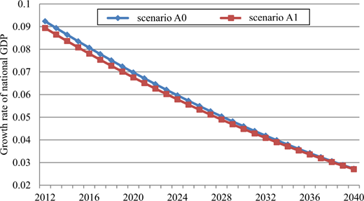
Table III shows the GDP growth of eight regions for the two scenarios. Based on the simulation results, there is a common result of the scenarios. That is, compared with the national average growth rate, the GDP growth rate of the southeast coastal region and the new type of industrializing area is higher than the national average growth rate; the GDP growth rate of the Circum-Bohai-Sea region, the Yangtze River Delta region, the energy base region, the classic industrial base region and the industrialized region are lower than the national average growth rate; the GDP growth rate of the environmentally fragile region does not significantly differ from the national average growth rate. Thus, according to our results, the GDP growth rate of the more economically developed regions is slow, whereas the GDP growth rate of the less economically developed regions is fast.
Regional GDP growth rate for the two scenarios
| Scenario | Year | 2012 | 2020 | 2025 | 2030 | 2035 | 2040 |
|---|---|---|---|---|---|---|---|
| A0 | Circum-Bohai-Sea region | 0.0806 | 0.0642 | 0.0552 | 0.0447 | 0.0346 | 0.0262 |
| Yangtze River Delta region | 0.0801 | 0.0629 | 0.0539 | 0.0431 | 0.0333 | 0.0248 | |
| Southeast coastal region | 0.1240 | 0.0862 | 0.0680 | 0.0540 | 0.0454 | 0.0381 | |
| Energy base region | 0.0780 | 0.0614 | 0.0528 | 0.0425 | 0.0337 | 0.0245 | |
| Classic industrial base region | 0.0772 | 0.0617 | 0.0533 | 0.0435 | 0.0343 | 0.0255 | |
| Industrialized region | 0.0738 | 0.0586 | 0.0510 | 0.0416 | 0.0334 | 0.0252 | |
| Industrializing region | 0.0995 | 0.0717 | 0.0587 | 0.0492 | 0.0414 | 0.0350 | |
| Environmentally fragile region | 0.0827 | 0.0649 | 0.0554 | 0.0460 | 0.0359 | 0.0269 | |
| A1 | Circum-Bohai-Sea region | 0.0761 | 0.0600 | 0.0538 | 0.0421 | 0.0329 | 0.0251 |
| Yangtze River Delta region | 0.0789 | 0.0620 | 0.0525 | 0.0410 | 0.0327 | 0.0242 | |
| Southeast coastal region | 0.1252 | 0.0875 | 0.0755 | 0.0608 | 0.0486 | 0.0374 | |
| Energy base region | 0.0785 | 0.0622 | 0.0564 | 0.0446 | 0.0387 | 0.0265 | |
| Classic industrial base region | 0.0777 | 0.0622 | 0.0556 | 0.0446 | 0.0362 | 0.0264 | |
| Industrialized region | 0.0679 | 0.0531 | 0.0491 | 0.0374 | 0.0300 | 0.0232 | |
| Industrializing region | 0.0933 | 0.0694 | 0.0579 | 0.0463 | 0.0382 | 0.0271 | |
| Environmentally fragile region | 0.0860 | 0.0664 | 0.0570 | 0.0465 | 0.0367 | 0.0272 |
Compared with the simulation results of Scenarios A0 and A1, the GDP growth rates of the emigrating population regions – the Circum-Bohai-Sea region, the Yangtze River Delta region, the industrialized region and the industrializing region – are lower than the GDP growth rate of the baseline scenario. The reduction ratio is between 0.79 and 0.1 per cent. In addition, the decreasing rate of GDP growth rate reflects a trend of gradual transition over time. That is, the impact of migration on GDP gradually weakens over time. The migration scale also influences the change trend of the GDP growth rate. The industrializing region has the largest emigrating population, followed by the industrialized region and the Circum-Bohai-Sea Region. The Yangtze River Delta region has the smallest emigrating population. Compared with the other three regions, in the preceding four regions, the downward GDP growth rate trend of the industrializing region is obvious. The least influenced region on GDP is the Yangtze River Delta region. The simulation results for immigrating regions are opposite for the emigrating regions. The southeast coastal region, the energy base region, the classic industrial base region and the environmentally fragile region are immigrating-population regions. The GDP growth rates of these regions are higher than the GDP growth rate of the baseline scenario. The reduction ratio is between 0.75 and 0.09 per cent. In addition, the increasing rate of GDP growth exhibits a trend toward a gradual transition over time. That is, the impact of migration on GDP gradually weakens over time. Similarly, the migration scale also influences the change trend of the GDP growth rate. The southeast coastal region has the largest immigrating population, followed by the environmentally fragile region and the energy base region. The classic industrial base region has the smallest emigrating population. Compared with the other three regions, among the preceding four regions, the GDP growth rate of the southeast coastal region increases the most. The area that experiences the least impact on its GDP has the smallest migration scale: the classical industrial base region.
Table IV shows per-capita GDP for the two scenarios. In both scenarios, the per-capita GDP exhibits an increasing trend. However, because of labor migration, the increase in emigration and immigration differs from the baseline scenario. It can be observed that the Circum-Bohai-Sea region, the Yangtze River Delta region, the industrialized region and the industrializing region are emigrating-population regions. In the baseline scenario, the per-capita GDP of these four regions is lower than the per-capita GDP in Scenario A1. The remaining four regions are immigrating-population regions. In the baseline scenario, the per-capita GDP of these regions is higher than the per-capita GDP in Scenario A1. Although migration increases the economic-development speed of the immigrating-population regions, the acceleration of economic development remains lower than the speed of population migration, with the result that the per-capita GDP is lower than that of the baseline scenario. However, although the GDP development rate of a migrating-population region slows, the decline magnitude of the population is larger than that of GDP growth. Therefore, the per-capita GDP of the emigrating-population regions increases rather than decreases.
Regional per-capita GDP for the two scenarios unit: Yuan 10,000
| Scenario | Year | 2012 | 2020 | 2025 | 2030 | 2035 | 2040 |
|---|---|---|---|---|---|---|---|
| A0 | Circum-Bohai-Sea region | 4.668 | 8.381 | 12.195 | 17.744 | 25.817 | 37.563 |
| Yangtze River Delta region | 4.738 | 8.587 | 12.556 | 18.361 | 26.848 | 39.260 | |
| Southeast coastal region | 5.510 | 15.230 | 27.202 | 48.583 | 86.772 | 154.977 | |
| Energy base region | 1.391 | 2.528 | 3.659 | 5.298 | 7.670 | 11.104 | |
| Classic industrial base region | 2.361 | 6.038 | 9.900 | 16.233 | 26.617 | 43.643 | |
| Industrialized region | 1.883 | 3.256 | 4.620 | 6.557 | 9.304 | 13.204 | |
| Industrializing region | 2.287 | 5.173 | 8.236 | 13.111 | 20.873 | 33.230 | |
| Environmentally fragile region | 1.361 | 2.677 | 3.780 | 5.338 | 7.537 | 10.642 | |
| A1 | Circum-Bohai-Sea region | 4.796 | 9.063 | 13.588 | 20.373 | 30.545 | 45.797 |
| Yangtze River Delta region | 4.741 | 8.584 | 12.552 | 18.354 | 26.839 | 39.247 | |
| Southeast coastal region | 5.193 | 12.887 | 20.516 | 32.661 | 51.997 | 82.780 | |
| Energy base region | 1.377 | 2.411 | 3.456 | 4.954 | 7.101 | 10.177 | |
| Classic industrial base region | 2.354 | 4.146 | 5.942 | 8.517 | 12.208 | 17.498 | |
| Industrialized region | 1.925 | 3.562 | 5.055 | 7.174 | 10.180 | 14.446 | |
| Industrializing region | 2.351 | 5.626 | 9.230 | 15.142 | 24.840 | 40.750 | |
| Environmentally fragile region | 1.324 | 2.422 | 3.421 | 4.830 | 6.820 | 9.629 |
In sum, the migration caused by climate change has slowed the speed of national economic development. The influence of migration on a region is related to the migration’s direction. Migration increases the GDP growth rate of immigrating-population regions and decreases the GDP growth rate of emigrating-population regions. However, the change in per-capita GDP is the opposite. The per-capita GDP of immigrating-population regions is lower than that of the baseline scenario, whereas the per-capita GDP of emigrating-population regions is higher than that of the baseline scenario. In addition, the larger the migration is, the larger the impact on the regional economy. Subsequently, the impact of migration on the economy gradually weakens over time.
3.2.2 Income and consumption impact.
Table V shows the change in resident income growth rate for the entire country and the regions for the two scenarios. The change in resident income growth for the entire country is analyzed as following. Comparing Scenario A0 with Scenario A1, it can be observed that the resident income growth rate for the entire country gradually decreases. However, compared with the resident income growth rate of the baseline scenario, the resident income growth rate of Scenario A1 is slower. That is, migration can slow the resident income growth rate. In addition, during the early stage of simulation, the results for Scenario A1 exhibit the largest difference from those for the baseline scenario. The difference between the two scenarios with respect to the resident income growth rate becomes increasingly smaller over time.
Regional income growth rate for the two scenarios
| Scenario | Year | 2012 | 2020 | 2025 | 2030 | 2035 | 2040 |
|---|---|---|---|---|---|---|---|
| A0 | Circum-Bohai-Sea region | 0.0750 | 0.0597 | 0.0513 | 0.0416 | 0.0322 | 0.0244 |
| Yangtze River Delta region | 0.0745 | 0.0585 | 0.0501 | 0.0401 | 0.0310 | 0.0231 | |
| Southeast coastal region | 0.1153 | 0.0801 | 0.0632 | 0.0502 | 0.0422 | 0.0355 | |
| Energy base region | 0.0726 | 0.0571 | 0.0491 | 0.0395 | 0.0313 | 0.0228 | |
| Classic industrial base region | 0.0718 | 0.0574 | 0.0496 | 0.0405 | 0.0319 | 0.0237 | |
| Industrialized region | 0.0686 | 0.0545 | 0.0474 | 0.0387 | 0.0311 | 0.0234 | |
| Industrializing region | 0.0925 | 0.0667 | 0.0546 | 0.0457 | 0.0385 | 0.0325 | |
| Environmentally fragile region | 0.0769 | 0.0594 | 0.0506 | 0.0418 | 0.0325 | 0.0241 | |
| Entire country | 0.0856 | 0.0646 | 0.0530 | 0.0425 | 0.0332 | 0.0251 | |
| A1 | Circum-Bohai-Sea region | 0.0708 | 0.0558 | 0.0500 | 0.0392 | 0.0306 | 0.0234 |
| Yangtze River Delta region | 0.0733 | 0.0576 | 0.0488 | 0.0382 | 0.0304 | 0.0225 | |
| Southeast coastal region | 0.1164 | 0.0814 | 0.0702 | 0.0565 | 0.0452 | 0.0348 | |
| Energy base region | 0.0730 | 0.0578 | 0.0524 | 0.0415 | 0.0360 | 0.0246 | |
| Classic industrial base region | 0.0723 | 0.0578 | 0.0517 | 0.0415 | 0.0337 | 0.0246 | |
| Industrialized region | 0.0631 | 0.0494 | 0.0457 | 0.0348 | 0.0279 | 0.0215 | |
| Industrializing region | 0.0867 | 0.0646 | 0.0538 | 0.0431 | 0.0356 | 0.0252 | |
| Environmentally fragile region | 0.0800 | 0.0618 | 0.0512 | 0.0395 | 0.0313 | 0.0240 | |
| Entire country | 0.0831 | 0.0628 | 0.0517 | 0.0417 | 0.0328 | 0.0250 |
By observing the resident income growth in each region, it is found that three regions, namely, the southeast coastal region, the industrializing region and the environmentally fragile region, exhibit a faster income growth rate in the two scenarios. In addition, the simulation results for the resident income growth rate of the Circum-Bohai-Sea region, the Yangtze River Delta region, the industrialized region and the industrializing region in Scenario A0 is higher than in Scenario A1. Notably, these four regions are emigration regions. Obviously, an emigrating population is unfavorable to an increase in the resident income growth rate. If continuing to observe the difference in the change in resident income in the two scenarios, it is also found that the resident income growth rates gradually converge. That is, the longer that the period is, the smaller the impact of migration policy on resident income and the weaker the policy effect. The remaining regions are immigration regions. In these regions, the simulation result for the resident income growth rate in Scenario A0 is lower than that in Scenario A1. This result can be considered to be a result of immigration. That is, immigration increases the income of residents. Similarly, over time, income range of increase also gradually decreases.
Table VI shows the change in the resident consumption growth rate for the entire country and the regions for the two scenarios. The trend and characteristics of the change in resident consumption are coincident with the change circumstances for resident income (Table V). The simulation result for the change rate of resident consumption growth in an emigrating population in Scenario A0 is higher than that in Scenario A1. The simulation result for the change rate of resident consumption growth in an immigrating population in Scenario A0 is lower than that in Scenario A1. With time, the impact of migration policy on resident income becomes increasingly smaller. In addition, the consumption growth rate is always lower than the income growth rate. As mentioned in a previous paper, income influences consumption and the propensity to consume primarily depends on the income amount. That is, consumption increases as income increases. However, the increase in consumption is lower than the increase in income.
Regional consumption growth rate for the two scenarios
| Scenario | Year | 2012 | 2020 | 2025 | 2030 | 2035 | 2040 |
|---|---|---|---|---|---|---|---|
| A0 | Circum-Bohai-Sea region | 0.0726 | 0.0578 | 0.0497 | 0.0403 | 0.0311 | 0.0236 |
| Yangtze River Delta region | 0.0721 | 0.0567 | 0.0485 | 0.0388 | 0.0300 | 0.0224 | |
| Southeast coastal region | 0.1116 | 0.0775 | 0.0612 | 0.0486 | 0.0409 | 0.0343 | |
| Energy base region | 0.0702 | 0.0553 | 0.0475 | 0.0382 | 0.0303 | 0.0221 | |
| Classic industrial base region | 0.0695 | 0.0555 | 0.0480 | 0.0392 | 0.0309 | 0.0230 | |
| Industrialized region | 0.0664 | 0.0528 | 0.0459 | 0.0374 | 0.0301 | 0.0227 | |
| Industrializing region | 0.0896 | 0.0645 | 0.0528 | 0.0443 | 0.0372 | 0.0315 | |
| Environmentally fragile region | 0.0744 | 0.0575 | 0.0490 | 0.0405 | 0.0314 | 0.0233 | |
| Entire country | 0.0829 | 0.0626 | 0.0513 | 0.0412 | 0.0322 | 0.0243 | |
| A1 | Circum-Bohai-Sea region | 0.0685 | 0.0540 | 0.0484 | 0.0379 | 0.0296 | 0.0226 |
| Yangtze River Delta region | 0.0710 | 0.0558 | 0.0472 | 0.0369 | 0.0294 | 0.0218 | |
| Southeast coastal region | 0.1127 | 0.0788 | 0.0679 | 0.0547 | 0.0438 | 0.0336 | |
| Energy base region | 0.0707 | 0.0560 | 0.0507 | 0.0402 | 0.0349 | 0.0238 | |
| Classic industrial base region | 0.0699 | 0.0559 | 0.0501 | 0.0401 | 0.0326 | 0.0238 | |
| Industrialized region | 0.0611 | 0.0478 | 0.0442 | 0.0337 | 0.0270 | 0.0208 | |
| Industrializing region | 0.0839 | 0.0625 | 0.0521 | 0.0417 | 0.0344 | 0.0244 | |
| Environmentally fragile region | 0.0774 | 0.0598 | 0.0495 | 0.0382 | 0.0303 | 0.0241 | |
| Entire country | 0.0802 | 0.0606 | 0.0498 | 0.0401 | 0.0315 | 0.0241 |
Table VII shows the change in resident per-capita income growth rate in each region for the two scenarios. It can be concluded that the simulation result for the resident per-capita income growth rate for an emigrating population in Scenario A0 is higher than that in Scenario A1. Over time, the resident income growth rate gradually converges. That is, the longer that the period is, the smaller the impact of migration policy on resident income and the weaker the policy effect. The simulation result for the resident income growth rate for an immigrating population in Scenario A0 is lower than that in Scenario A1. Immigration decreases the increasing magnitude of resident per-capita income growth. Similarly, over time, the decreasing magnitude of the income increase also gradually narrows. Table VIII shows the change in the resident per-capita consumption growth rate in each region for the two scenarios. The trend and characteristics of the change in resident per-capita consumption are coincident with the change in resident income (Table VII). The resident per-capita consumption growth rate in the baseline scenario is higher than that in Scenario A1. The simulation result for the resident per-capita consumption growth rate in an emigrating population in Scenario A0 is higher than that in Scenario A1. The simulation result for the resident per-capita consumption growth rate in an immigrating population in Scenario A0 is lower than that in Scenario A1. Over time, the impact of migration policy on resident income becomes increasingly smaller. Through the change in resident income and resident consumption, the distribution of the population pattern caused by climate change overall decreases the increasing magnitude of these two variables. Based on the simulation results for the regional growth rate, the migration direction affects resident income and resident consumption. Relative to the baseline scenario, the change rates of consumption and income in emigrating-population regions decrease, whereas, in immigrating-population regions, they increase. In addition, the impact of migration on income and consumption gradually weakens.
Regional per-capita income growth for the two scenarios
| Scenario | Year | 2012 | 2020 | 2025 | 2030 | 2035 | 2040 |
|---|---|---|---|---|---|---|---|
| A0 | Circum-Bohai-Sea region | 0.0600 | 0.0478 | 0.0411 | 0.0333 | 0.0257 | 0.0195 |
| Yangtze River Delta region | 0.0596 | 0.0468 | 0.0401 | 0.0321 | 0.0248 | 0.0185 | |
| Southeast coastal region | 0.0923 | 0.0641 | 0.0506 | 0.0402 | 0.0338 | 0.0284 | |
| Energy base region | 0.0581 | 0.0457 | 0.0393 | 0.0316 | 0.0251 | 0.0183 | |
| Classic industrial base region | 0.0574 | 0.0459 | 0.0397 | 0.0324 | 0.0255 | 0.0190 | |
| Industrialized region | 0.0549 | 0.0436 | 0.0379 | 0.0309 | 0.0248 | 0.0187 | |
| Industrializing region | 0.0740 | 0.0533 | 0.0437 | 0.0366 | 0.0308 | 0.0260 | |
| Environmentally fragile region | 0.0615 | 0.0475 | 0.0405 | 0.0335 | 0.0260 | 0.0193 | |
| A1 | Circum-Bohai-Sea region | 0.0566 | 0.0447 | 0.0400 | 0.0314 | 0.0245 | 0.0187 |
| Yangtze River Delta region | 0.0587 | 0.0461 | 0.0391 | 0.0305 | 0.0243 | 0.0180 | |
| Southeast coastal region | 0.0931 | 0.0651 | 0.0561 | 0.0452 | 0.0362 | 0.0278 | |
| Energy base region | 0.0584 | 0.0463 | 0.0419 | 0.0332 | 0.0288 | 0.0197 | |
| Classic industrial base region | 0.0578 | 0.0462 | 0.0414 | 0.0332 | 0.0269 | 0.0197 | |
| Industrialized region | 0.0505 | 0.0395 | 0.0366 | 0.0278 | 0.0223 | 0.0172 | |
| Industrializing region | 0.0694 | 0.0517 | 0.0431 | 0.0344 | 0.0285 | 0.0202 | |
| Environmentally fragile region | 0.0640 | 0.0494 | 0.0409 | 0.0316 | 0.0250 | 0.0199 |
Regional per-capita consumption growth for the two scenarios
| Scenario | Year | 2012 | 2020 | 2025 | 2030 | 2035 | 2040 |
|---|---|---|---|---|---|---|---|
| A0 | Circum-Bohai-Sea region | 0.0581 | 0.0462 | 0.0397 | 0.0322 | 0.0249 | 0.0189 |
| Yangtze River Delta region | 0.0577 | 0.0453 | 0.0388 | 0.0311 | 0.0240 | 0.0179 | |
| Southeast coastal region | 0.0893 | 0.0620 | 0.0490 | 0.0389 | 0.0327 | 0.0275 | |
| Energy base region | 0.0562 | 0.0442 | 0.0380 | 0.0306 | 0.0243 | 0.0177 | |
| Classic industrial base region | 0.0556 | 0.0444 | 0.0384 | 0.0314 | 0.0247 | 0.0184 | |
| Industrialized region | 0.0531 | 0.0422 | 0.0367 | 0.0299 | 0.0240 | 0.0181 | |
| Industrializing region | 0.0716 | 0.0516 | 0.0422 | 0.0354 | 0.0298 | 0.0252 | |
| Environmentally fragile region | 0.0595 | 0.0460 | 0.0392 | 0.0324 | 0.0252 | 0.0186 | |
| A1 | Circum-Bohai-Sea region | 0.0548 | 0.0432 | 0.0387 | 0.0303 | 0.0237 | 0.0181 |
| Yangtze River Delta region | 0.0568 | 0.0446 | 0.0378 | 0.0296 | 0.0235 | 0.0174 | |
| Southeast coastal region | 0.0901 | 0.0630 | 0.0543 | 0.0437 | 0.0350 | 0.0269 | |
| Energy base region | 0.0565 | 0.0448 | 0.0406 | 0.0321 | 0.0279 | 0.0191 | |
| Classic industrial base region | 0.0560 | 0.0448 | 0.0401 | 0.0321 | 0.0261 | 0.0190 | |
| Industrialized region | 0.0489 | 0.0382 | 0.0354 | 0.0269 | 0.0216 | 0.0167 | |
| Industrializing region | 0.0672 | 0.0500 | 0.0417 | 0.0333 | 0.0275 | 0.0195 | |
| Environmentally fragile region | 0.0619 | 0.0478 | 0.0396 | 0.0306 | 0.0242 | 0.0193 |
3.2.3 Change in regional disparity.
In this paper, the regional disparity index characterized by the Theil coefficient is applied to analyze the change in regional disparity. In Equation (42), I0(x) is the total regional Theil coefficient, which reflects the total regional disparity. xi is the total GDP of a region i. x̄ is the mean value of all regional GDP and n is the region number (Shorrocks, 1980, 1984):
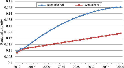
Figure 2 shows the total regional disparity change represented by the Theil coefficient of the GDP. In the baseline scenario, the total regional disparity gradually expands from 0.109 in 2012 to 0.145 in 2040, and the expansion range is 0.036. When migration increases, regional disparity gradually increases. However, the increased range is smaller than in the baseline scenario. From 2012 to 2040, the regional disparity increases by 0.016. Obviously, the migration scenario can decrease the expansion speed of regional disparity. Although the difference in the total regional disparity in the two scenarios gradually increases, the expansion speed gradually decreases.
In addition, regional disparity can be divided into inner-regional disparity change and inter-regional disparity. Equation (42) expresses the total regional disparity, which is the sum of inner-regional disparity and inter-regional disparity. This paper uses A. F. Shorrocks’s method to decompose the overall Theil coefficient. The left side of equation (43) is the total regional Theil coefficient. The first item on the right side of the equation is the Theil coefficient within regions, and the second item is the Theil coefficient among regions. K is the number of divisions by region, pk is the proportion of the population in Group k of the total population and vk is the proportion of GDP in Group k in GDP of the whole country:
Figure 3 shows the inner-regional disparity change. First, the change in inner-regional disparity is analyzed. Whether in the baseline scenario or the migration scenario, inner-regional disparity gradually expands over time. However, it must be noted that the simulation result for inner-regional disparity change in the migration scenario is smaller than that in the natural scenario, which contrasts with the overall regional disparity. In the baseline scenario, the inter-regional disparity in 2040 expands to 0.0224 by the end of the simulation. After migration is added, the inter-regional disparity in 2040 is 0.0226. Compared with the baseline scenario, the inner-regional disparity change in the migration scenario improves by 0.9 percentage points. Obviously, although migration decreases total regional disparity, it can expand regional disparity. In addition, compared with 2012, regional disparity in the baseline scenario expands by 0.0057 in 2040, whereas regional disparity in the migration scenario expands by 0.0058 in 2040. Overall, regional disparity in the two scenarios gradually expands over time. However, the growth rate gradually decreases.
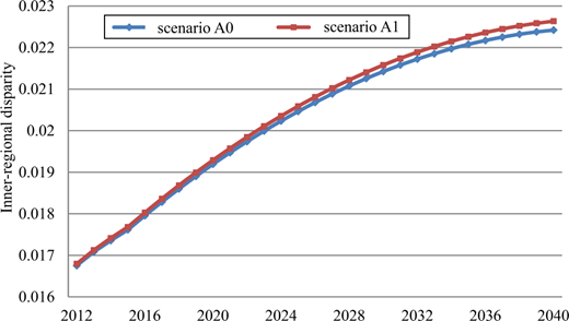
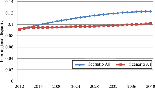
Figure 4 shows the change in inter-regional disparity. Overall, the trend of inter-regional disparity is consistent with overall regional disparity. The inter-regional disparity gradually expands over time. The inter-regional disparity in the baseline scenario is larger than that in the migration scenario. The difference in the inter-regional disparity between the two scenarios gradually expands. However, the difference between expansion speeds gradually narrows. When inner-regional disparity and inter-regional disparity are combined, migration decreases inter-regional disparity and expands inner-regional disparity. However, the decrease in inter-regional disparity can cause inner-regional disparity to expand. The final result of the combination of the two is that overall regional disparity is decreased.
In sum, migration expands inner-regional disparity and decreases inter-regional disparity. The overall regional disparity is decreased. Subsequently, migration causes the difference in the regional disparity in the two scenarios to expand. However, the expansion speed gradually decreases.
4. Conclusions
In this paper, a climate change economic model which combined a population migration model based on potential agricultural production with a dynamic multi-regional CGE model is introduced. This new framework can be applied to analysis population migrations induced by climate change and the corresponding social-economic effects.
The results reveal that in response to climate change the regions that will probably experience population emigration are primarily the Circum-Bohai-Sea region, the industrialized region, the industrializing region and the Yangtze River Delta region. Specifically, the emigrating population in the first three regions will account for 99 per cent of that of the entire country. The remaining four regions are immigration regions: the Southeast coastal region, the energy base region, the environmentally fragile region and the classic industrial base region. Based on the ratio of the emigrating and immigrating populations and the regional population, the proportion of the immigrating population in the southeast coastal region has exceeded 30 per cent of the local area’s total population, whereas the proportion of the migration population in the Yangtze River Delta region and the classic industrial base region is less than 3 per cent, whereby the proportion of the emigrating population is the lowest (0.37 per cent). Based on the research results, under the condition of a rapidly aging population, the Circum-Bohai-Sea region, the industrialized region and the industrializing region will face a severe labor shortage, which will affect economic development. As soon as possible, policies must be developed to encourage and attract skilled labor.
Based on the impact of migration on the economy, the migration caused by climate change will increase the GDP growth rate of immigration regions and decrease the GDP growth rate of emigration regions. The larger the migration is, the larger its impact is on the regional economy. However, overall, the GDP growth rate of the entire country will slow. Climate change can result in a population redistribution, which will decrease the range of resident income and resident consumption. Notably, migration can expand inter-regional disparity and decrease inner-regional disparity. However, the total effect of the two gap effects will ultimately help decrease overall regional disparity.
It should be noted that the effect of migration in response to climate change on potential agricultural production is not a prediction but only to advance a possibility of population migration adapting to climate change. In fact, if transportation conditions and migration viscosity are considered, generally, cross-regional food mobilization is preferable to migration unless extreme climate change results in a catastrophic decrease in potential agricultural production. Of course, this statement does not mean that the impact of climate change on population distribution can be ignored. If the indirect effect exerted by the economic system is superimposed, future large-scale Chinese migration will continue to be an unavoidable problem.
Note
In this model and the following model, subscript 1 represents the baseline year, subscript 2 represents the target year and subscript j represents area j.
The authors are grateful to anonymous reviewers for their heuristic comments. Opinions are those of the authors. Research funding provided by National Natural Science Foundation (41271551, 71201157), National 973 Project (2012CB955800) and Key Project of the CAS (XDA05150900) are gratefully acknowledged.
