Time-varying impact of monetary policy on the macroeconomy in Sri Lanka

As an emerging economy, Sri Lanka has received widespread attention due to its unique geographical location and economic potential. The Sri Lankan economy experienced rapid development in the latter half of the 20th and early 21st centuries, driven by key sectors including agriculture, manufacturing and services. However, the onset of the civil war profoundly affected the nation's economy, leading to the squandering of resources, infrastructure damage and the loss of human capital. After the civil war ended in 2009, the Sri Lankan government implemented large-scale reconstruction measures, particularly in infrastructure and tourism, which have stimulated economic recovery to a certain extent. Nevertheless, some challenges still need to be addressed, including high inflation, insufficient foreign exchange reserves, mounting trade deficits and a growing national debt (Choudhary, 2022; Nimal and Namboodiripad, 2022).

Sri Lanka is a small open economy with an unstable economic structure, making it vulnerable to external shocks (Naranpanawa and Bandara, 2012). The 2019 Easter terrorist attacks and the COVID-19 pandemic severely hit Sri Lanka's tourism industry, causing the economic situation to deteriorate rapidly. Meanwhile, the domestic organic farming policy failed, and the Russian–Ukrainian war had adverse effects on oil and food prices, ultimately leading to sharp increases in consumer prices. Specifically, economic growth turned negative in 2020, and price levels in the second half of 2022 increased by more than 50% year on year. Against this backdrop, the Central Bank of Sri Lanka (CBSL) shifted its Monetary Policy (MP) stance toward tightening to combat inflation, soaring market interest rates and dwindling foreign exchange reserves.

Under the Monetary Law Act, the CBSL has comprehensive responsibility and authority in achieving economic, price and financial stability. The CBSL introduced Flexible Inflation Targeting (FIT) in 2020, prioritizing price stability while supporting economic growth and maintaining flexible exchange rate management ^[1]. However, soon after the introduction of FIT, the COVID-19 pandemic and the subsequent economic crisis in 2022 made it difficult for the framework to be fully implemented. In particular, the CBSL implemented a managed floating exchange rate regime to reduce exchange rate fluctuations. Notably, from the latter half of 2021 to the first half of 2022, the CBSL conducted extensive market interventions. It is evident that Sri Lanka's economic development is facing severe challenges, and the unprecedented crisis makes the role of MP in macroeconomics even more critical.

However, the MP of CBSL appears to lack effectiveness, particularly concerning the average weighted call money rate (AWCMR), a short-term interest rate that has exhibited extreme instability. Meanwhile, an increase in money supply exacerbated financial sector instability, affecting the entire macroeconomic system. Therefore, we decided to explore how Sri Lanka's MP affects its macroeconomy. This will not only help policymakers better understand the consequences of policy decisions but also provide targeted recommendations for improving Sri Lanka's economic conditions. Furthermore, Sri Lanka's MP experience can provide useful lessons and inspiration for other developing countries dealing with similar economic challenges.

Since MP instruments cannot individually adjust macroeconomy, systematic comparative analysis becomes particularly critical. Therefore, we examine the multilevel effects of MP on real GDP, inflation, stock markets, exchange rates and market interest rates, which can provide a reference for policymakers facing trade-offs between economic growth, price levels and financial system stability. Additionally, given the ever-changing characteristics of economic conditions, traditional constant coefficient models cannot identify time-varying impacts of policy shocks on the macroeconomy (Bringmann et al., 2018; Ding et al., 2021; Huang et al., 2021). To address this limitation, we employ a novel time-varying parameter vector autoregression (TVP-VAR) approach that allows the variance-covariance matrices and coefficients to change over time, thereby capturing nonlinear, complex, time-varying interrelationships between variables.

This paper makes the following main contributions. First, this paper is the first to explore the time-varying impact of MP on Sri Lanka's macroeconomy. Second, our research covers a longer time span compared with existing studies, including the impact of MP after the COVID-19 outbreak. Third, utilizing the TVP-VAR method, we capture time-varying responses of Sri Lanka's macroeconomics to MP shock at different time scales and employ impulse responses at different time points to enrich the research results further.

The remainder of the paper is organized as follows: Section 2 reviews the literature; Section 3 specifies the methodology and data; Section 4 discusses the empirical results; and Section 5 concludes the paper.

Early research on the relationships between MP and macroeconomics mainly focused on developed countries (Christiano et al., 1999; Gaiotti and Generale, 2002; Sims, 1992). Bernanke and Blinder (1992) are the first to introduce the vector autoregression (VAR) models to analyze US MP shocks. They find that the federal fund rate can significantly influence bank deposits, subsequently impacting the real economy. Taylor (1995) extends the analysis to seven major developed countries, revealing a long-term stable relationship between interest rates and macroeconomic variables such as investment, consumption and economic growth. Furthermore, Mountford (2005) argues that UK MPs exert a limited influence on macroeconomic variables, but this contradicts the conclusion of Cloyne and Hürtgen (2016), who find that a rise in UK policy rates causes a reduction in output and inflation. Subsequently, Champagne and Sekkel (2018) confirm that the impact of Canada's MP on output is consistent with that in the UK (Cloyne and Hürtgen, 2016), but the impact on inflation is considerably weaker.

Due to underdeveloped financial structures, MP outcomes in emerging countries exhibit considerable heterogeneity (Laurens, 2005; Mishra and Montiel, 2013). Ülke and Berument (2016) focus on Turkey and find that tight MP reduces the exchange rate, prices and output. Furthermore, a tighter MP has a stronger shock to the economy than a loose MP. Afrin (2017) finds that MP effectively affects prices in Bangladesh, and bank lending channels play a more critical role in the transmission process than the exchange rate channel. Based on the structural VAR framework, Anwar and Nguyen (2018) found that although MP significantly impacts economic growth in Vietnam, it remains susceptible to external shocks. Munir (2018) argues that MP serves as an effective measure to control price levels in Pakistan and has a real effect on output in the short term. In addition, after controlling for international factors, including oil price and global interest rate, Dua and Tuteja (2023) find that India's tightening MP can suppress inflation with a negligible impact on output.

Existing studies on the effect of MP on Sri Lanka's macroeconomics are relatively limited and mainly rely on the traditional VAR framework. Based on data from 1978 to 2005, Amarasekara (2008) finds that contractionary MP leads to appreciation of exchange rates, lower inflation and output growth in Sri Lanka. Maitra and Debnath (2015) further extended the time horizon to include the 2008 global financial crisis and found that Sri Lanka's MP is effective during such crises. In alignment with theoretical expectations, raising interest rates stabilizes the price level but depresses income, and increasing the money supply causes price levels and incomes to rise. Abeygunawardana et al. (2017) argue that policy interest rates strongly impact money and government securities market rates but have a weaker impact on prices and the real sector. Furthermore, they reveal that factors including excess market liquidity, the underground economy and shallow financial markets constrain the effective transmission of MP in Sri Lanka. The latest research conducted by Hansi (2023) shows that interest rates have a negative effect on the exchange rate and output, while money supply growth positively affects output with an insignificant impact on inflation.

On the other hand, several studies have investigated the transmission channels and the effectiveness of MP in Sri Lanka. Using several VAR models, Ghazanchyan (2014) finds that the bank lending and interest rate channels play a more critical role than exchange rates and asset price channels in the transmission process of Sri Lanka's MP. However, Perera (2016) argues that MP affects output and price levels in Sri Lanka equally effectively through exchange rates, asset prices and bank credit channels. Musthafa et al. (2023) confirm that MP significantly impacts the macroeconomics in Sri Lanka and reveals the phenomena of the “exchange rate puzzle” and “price puzzle.” Moreover, after the Sri Lankan civil war ended, contractionary MP effectively curbed inflation, with the exchange rates and interest rates channels playing a dominant role.

In summary, research on the relationships between MP shocks and macroeconomics in Sri Lanka is still limited. More importantly, the existing literature relies on the traditional VAR framework, which cannot capture the time-varying characteristics of MP shocks. Additionally, the data sets utilized are outdated and lack information after the COVID-19 outbreak. Therefore, to fill these gaps, this study collects data from 2006 to 2023 and examines the time-varying effects of MP on Sri Lanka's macroeconomy by constructing the TVP-VAR models.

Before introducing the TVP-VAR model, we define a VAR model:

where $yt$ represents a $k×1$ vector of endogenous variables. $A$ and $F1,⋯,Fs$ are $k×k$ coefficient matrix. $μt$ is the $k×1$ structural shocks and obeys $μt∼N(0,ΣΣ)$⁠, $Σ=diag(σ1,σ2,⋯,σk)$⁠. To simplify, consider structural shocks $A$ as lower triangular matrices, as defined by Equation (2):

Set $Bi=A−1F$ and $i=1,2,⋯,s$⁠, then Equation (1) is transformed into

where $εt$ represents the residual term, $Ik$ is the identity matrix and the elements in $Bi$ are converted into $ks2×1$-dimensional column vector $β$⁠. Meanwhile, assume $Xt=Ik⨂(yt−1′,⋯,yt−s′)$⁠, and $⨂$ is Kronecker product. Therefore, Equation (3) can be expressed as

Next, by introducing time-varying parameters into Equation (4), the TVP-VAR model with stochastic volatility is expressed as

where $βt$⁠, $At$ and $Σt$ all denote time-varying parameters. According to Nakajima (2011) and Primiceri (2005), the elements in the lower triangular matrices $At$ are restacked by rows into the vector $αt=(α21,α31,α41,⋯,αk,k−1)′$⁠, and define $ht=(h1t,h2t,⋯,hkt)′$⁠, with $hjt=log⁡σjt2,j=1,2,⋯,k;t=s+1,⋯,n$⁠. In order to reduce the estimated parameters, this paper assumes that time-varying parameters obey the random walk and are defined as follows:

where $t=s+1,⋯,n$⁠, $βs+1∼N(μβ0,Σβ0)$⁠, $αs+1∼N(μα0,Σα0)$ and $hs+1∼N(μh0,Σh0)$⁠. The shock of each time-varying parameter is independent, and $Σβ$⁠, $Σα$ and $Σh$ are all diagonal matrices.

Table 1 lists the definitions of variables adopted in this paper. We consider the AWCMR as a proxy for price-based MP, while reserve money (M0) and broad money (M2) represent quantity-based MP. The ultimate purpose of MP is to stabilize and promote macroeconomic development. Therefore, this paper chooses real GDP (realGDP), inflation (CPI) and stock market index (Stock) as proxy indicators of macroeconomic conditions. Furthermore, the market interest rate (MarketRate) and exchange rate (ExRate) are considered as channels to intuitively reflect the transmission mechanism of MP.

Our data set covers monthly observations from January 2006 to March 2023, and data availability limits the study period. It is worth noting that real GDP is available only quarterly or annually, making it unsuitable for direct comparison with other monthly variables or reflecting short-term macroeconomic fluctuations. To address this limitation, we utilize the global interpolation method to transform real GDP into monthly data. The raw data of AWCMR are daily data, which are transformed into monthly data after arithmetic mean processing. Furthermore, we use the Census-X12 method to seasonally adjust M0, M2, real GDP and CPI to remove the influence of seasonal factors. Finally, to ensure the stationarity of the data, AWCMR and market interest rate are differenced, and other variables are transformed into month-over-month growth rates for empirical analysis.

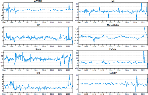
Figure 1 illustrates the dynamic changes of each variable, showing that all variables fluctuate around 0 without showing any apparent trends. This observation indicates that the processed data series exhibit stationarity. Additionally, there are differences in the magnitude of changes for variables over various time periods, with a notable increase in volatility during the COVID-19 pandemic. Given this context, opting for TVP-VAR models to capture nonlinear and time-varying relationships between the variables is a reasonable choice.

Table 2 reports the descriptive statistics and the results of three unit root tests for each variable. The skewness, kurtosis and Jarque–Bera statistics confirm that all series exhibit sharp peaks, fat tails and non-normality, while the Ljung–Box test reveals autocorrelation in all variables except M0 and Stock. The lower three rows report the Augmented Dickey–Fuller (ADF), Phillips–Perron (PP), and Elliott–Rothenberg–Stock (ERS) unit root test statistics. The null hypothesis of a unit root is rejected for every transformed series at conventional significance levels, confirming that all variables used in the TVP-VAR models are stationary.

This paper constructs three TVP-VAR models as follows: Model 1 (AWCMR, MarketRate, Stock, ExRate, CPI, realGDP), Model 2 (M0, MarketRate, Stock, ExRate, CPI, realGDP) and Model 3 (M2, MarketRate, Stock, ExRate, CPI, realGDP). To avoid overparameterization, the lag order for all models is set to 2 according to the Schwarz information criterion (SIC). Additionally, following the approach of Nakajima (2011), we employ Markov Chain Monte Carlo (MCMC) simulation for estimation, with the number of Gibbs sampling iterations set to 10,000.

Table 3 reports the parameter estimation results of the TVP-VAR models. It can be observed that the posterior means of each parameter lie within 95% confidence intervals. The diagnostic values of Geweke convergence are significantly smaller than a critical value of 1.96, indicating that parameters converge to posterior distributions at a 5% significance level. Additionally, all inefficiency factors generally have low values, with the highest value being only 105.98. In summary, the MCMC simulation of the TVP-VAR models is effective.

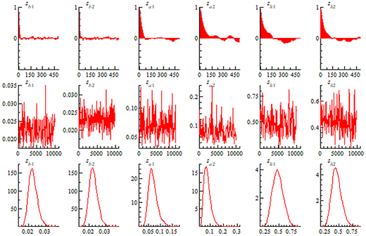
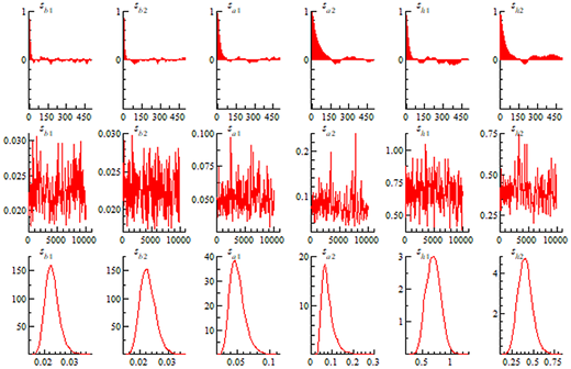
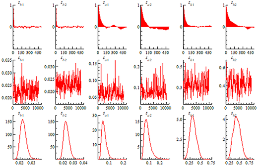
The dynamic simulation paths of the parameters in the three models are displayed in Figures 2–4. From top to bottom in each picture are the sample autocorrelation diagram, sample path and posterior density diagram. As the number of simulation increases, the autocorrelation coefficient of the samples gradually approaches zero, indicating that the correlation between the generated samples is eliminated. Furthermore, the sample path exhibits a “white noise” trajectory around the posterior mean, demonstrating that the MCMC method effectively simulates the parameter distribution. Finally, the sampling distribution significantly converges to posterior distributions, suggesting that the sample drawn is valid.

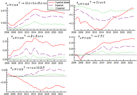
The TVP-VAR models can capture time-varying impulse responses. This study uses lag periods of 3, 6 and 12 months to investigate the short-term, medium-term and long-term effects of MP. Figure 5 illustrates the impulse responses of macroeconomic variables to AWCMR shock at various lag periods. AWCMR has a positive impact on market interest rates, with its intensity gradually increasing after 2008 and remaining stable after 2014. When AWCMR rises, it leads to higher borrowing costs for consumers and businesses, which pushes up market interest rates. Therefore, market interest rates play a critical role in the transmission of policy interest rates. Furthermore, the effect intensity gradually weakens as the lag period increases, meaning that the impact of AWCMR on the market interest rate is quickly transmitted and mainly concentrated in the short term.

A positive shock to AWCMR has a negative impact on the stock market in all periods. This is due to higher borrowing and financing costs as a result of rising AWCMR. Consequently, investments may decrease, and corporate performance could worsen, leading to a downturn in stock market performance. Additionally, AWCMR has a stronger negative impact on the stock market in the short term. However, post 2018, the negative impact on the short term has diminished compared to the medium and long term.

The exchange rate is measured as LKR per USD; therefore, an increase denotes depreciation of the Sri Lankan rupee. Under the conventional interest-differential channel, a rise in interest rates should attract capital inflows and lower the LKR-per-USD exchange rate (Frenkel, 2019). Our estimates instead show that a positive AWCMR shock raises the exchange rate, especially in the short term. In a highly indebted economy, tighter policy increases government and private-sector debt-service costs, weakens fiscal and balance-sheet positions and may raise sovereign-risk premiums. The resulting loss of confidence and capital-outflow pressure can outweigh the conventional interest-differential effect and depreciate the domestic currency. This mechanism is especially plausible for Sri Lanka, where public debt was assessed as unsustainable and foreign-exchange reserves were severely depleted during the crisis. Thus, the weak exchange-rate effect of AWCMR may reflect a fiscal-risk channel rather than a failure of the interest rate to affect market rates.

After 2009, the AWCMR shock led to an increase in inflation, which presented the “price puzzle.” The price puzzle is a common macroeconomic problem, referring to rising price levels caused by tight MP (Boivin and Giannoni, 2006; Champagne and Sekkel, 2018; Milcheva, 2013; Musthafa et al., 2023). Regarding the reasons for the price puzzle, Barth III and Ramey (2001) suggest that rising interest rates may cause deterioration of corporate credit conditions, thereby increasing marginal costs. Moreover, this result implies that after the civil war, CBSL adjustments to interest rates alone are insufficient to curb inflation.

While a positive shock to AWCMR has a short-term negative impact on real GDP, its effect tends to be zero in the long term. In the short term, increases in the CBSL interest rate lead to higher borrowing costs, restraining borrowing and consumption by businesses and individuals, negatively affecting overall economic activity and aggregate demand. However, in the long term, economic agents gradually adapt, mitigating the influence of interest rate hikes on economic growth.

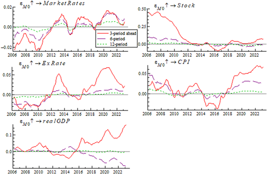
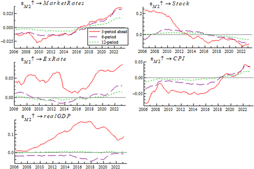
Figures 6 and 7 depict the impulse response of the macroeconomy to M0 and M2 shocks under various lag periods, respectively. Before 2012, M0 shocks had a negative impact on market interest rates, while after 2012, the impact became predominantly positive. The M2 shock initially caused market interest rates to fall, but after 2017, the impact of M2 on market interest rates reversed to positive. However, overall, the impact of M0 and M2 shocks on market interest rates appears insignificant as their values are very close to zero at different lag periods. Therefore, the market interest rate channel is insensitive to money supply shocks.

Initially, the increase in M0 and M2 positively impacts the stock market in the short term, which is consistent with the findings of Conrad (2021). However, the positive impact of M0 and M2 on the stock market after 2013 is minimal. The expansion of the money supply gives investors more capital to invest in stocks, leading to upward pressure on stock prices. Nevertheless, the impact could be limited if the economic outlook weakens or investors take a pessimistic view of the market. Additionally, the impact of M0 and M2 on the stock market remains insignificant in the medium and long term.

The positive response of the LKR-per-USD exchange rate to M0 shocks exhibits two short-term peaks, in 2013 and 2021, while the short-term response to M2 shocks remains positive. An expansion in money supply raises domestic liquidity and foreign-currency demand, thereby depreciating the rupee and increasing the LKR-per-USD rate. Therefore, the exchange rate is a critical short-term channel of quantity-based monetary policy.

Comparing the two policy measures reveals both a similarity and an important difference. AWCMR, M0 and M2 shocks all generate a positive short-run response of the LKR-per-USD exchange rate, but they operate through different mechanisms. AWCMR shocks are transmitted strongly to market interest rates; however, the conventional appreciation effect is offset by higher debt-service costs and sovereign-risk pressures. By contrast, M0 and M2 shocks have only small estimated effects on market interest rates, so their exchange-rate response is driven mainly by the direct liquidity and foreign-exchange-demand channels. Accordingly, the same directional exchange-rate response does not imply an identical transmission mechanism.

Except for the period from 2014 to 2018, M0 shocks caused inflation to rise most of the time. Therefore, controlling the growth of M0 is crucial to curb inflation and maintain price stability. Most M2 shocks have a negative impact on inflation most of the time, which contradicts the findings of Bala and Chin (2018). We speculate that this may be due to the unclear economic outlook in Sri Lanka. The growth of M2 indicates that companies and individuals are more inclined to save rather than consume and invest, which could exert a downward influence on inflation. It is worth noting that in recent years, the increase in M0 and M2 has had a strengthening impact on rising inflation.

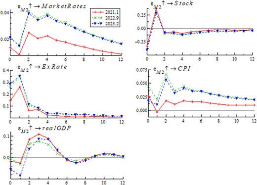
While both M0 and M2 have a positive impact on real GDP in the short term, these effects are either absent or even negative in the medium and long term. This result indicates that Sri Lanka's MP exhibits non-neutral characteristics. Increasing the money supply stimulates short-term economic growth, aligning with the conclusion of Hansi (2023), but its long-term impact is not significant.

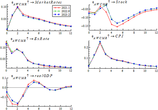
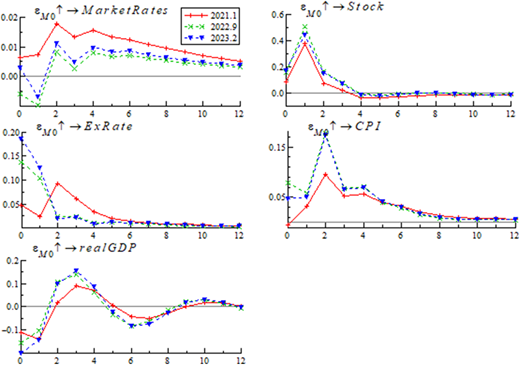
During the COVID-19 pandemic, the CBSL implemented accommodative MP measures to stimulate economic growth. However, this approach also led to a rise in inflation and economic instability. In response to this situation, after the pandemic, the CBSL adopted a tightening MP to address the lagged impact of the accommodative measures. Accordingly, this study selects January 2021, September 2022 and February 2023 as observation points, representing the initiation of interest rate hikes in Sri Lanka, the inflation peak and the most recent period, respectively. By comparing impulse responses at various time points, we aimed to evaluate the effectiveness of the tightening MP implemented after the epidemic.

Figures 8–10 illustrate impulse responses of the macroeconomy to MP shock at various time points. Specifically, at these three time points, the positive impact of all MPs on market interest rates and exchange rates reaches a peak within 2 months, gradually weakens and eventually approaches zero. The negative impact of AWCMR on the stock market reaches a trough after 5 months, while the positive impact of M0 and M2 on the stock market reaches a peak after 1 month. The response intensity of inflation to AWCMR shocks remains consistent at various time points. Furthermore, the effect of all MPs on real GDP is initially negative, then gradually turns positive and eventually approaches zero. In summary, the impact of Sri Lanka's MP on macroeconomics at the initiation of interest rate hikes, the inflation peak and the most recent period are similar in direction and duration, with slight differences in intensity. Therefore, we question the effectiveness of the tightening MP implemented in the wake of the COVID-19 pandemic.

Considering that the results of orthogonal impulse response may be different due to the order of endogenous variables, this study reorders the variables as follows: Model 1 (ExRate, Stock, CPI, AWCMR, MarketRate, realGDP), Model 2 (ExRate, M0, Stock, realGDP, CPI, MarketRate) and Model 3 (ExRate, Stock, M2, CPI, MarketRate, realGDP). Additionally, the lag length of the TVP-VAR model was adjusted to 4 according to the Akaike information criterion (AIC). The results of the impulse response analysis after changing the variable order and time lag are all very similar to the existing results ^[2].

This study uses Sri Lanka's data set from 2006 to 2023 to explore the time-varying effect of MP on the macroeconomy by establishing the TVP-VAR models. Specifically, we analyze the time-varying impacts of interest rates and money supply on inflation, economic growth and financial markets, as well as the transmission of market interest rates and exchange rate channels. Furthermore, we assess the effectiveness of tightening MP in the wake of the COVID-19 pandemic.

We find that Sri Lanka's MP exhibits significant time-varying and short-term effects on the macroeconomy, and the specific conclusions are as follows. First, the market interest rate channel plays a critical role in interest rate transmission, and the exchange rate is an important transmission channel for money supply in the short term. Second, a rise in interest rates typically causes stock prices to drop, while the impact of money supply on stock prices is not significant in most time periods. Third, after the civil war ended, inflation could not be effectively curbed by raising interest rates alone, and the “price puzzle” emerged. Conversely, controlling the growth of the money supply becomes increasingly important in maintaining price stability. Fourth, in the short term, rising interest rates inhibit economic growth, while increasing money supply stimulates economic growth. However, these effects gradually disappear in the long term. Finally, the effectiveness of tight MP implemented in the wake of the COVID-19 pandemic appears to be insignificant.

Based on the aforementioned findings and considering the current situation in Sri Lanka, this paper proposes the following policy recommendations. First, raising interest rates alone cannot effectively curb inflation. Instead, controlling the growth of the money supply is crucial for stabilizing the price level. The CBSL must closely monitor and control base monetary expansion to prevent excessive growth in the money supply. Second, given the short-term negative impact of interest rates on real GDP, fiscal policy tools can be employed to support economic growth during periods of interest rate increases. Although money supply has a short-term positive impact on real GDP, its long-term impact is limited. Therefore, the government should prioritize structural reforms, investments in human capital and infrastructure development to achieve sustained economic growth. Third, based on economic objectives, CBSL can adjust interest rates and money supply to achieve the expected market interest rate and exchange rate, which is crucial for investment and foreign trade. Finally, the government should improve transparency, market confidence and supervision to alleviate the negative effect of interest rate hikes on the stock market.

This study focuses on the market interest rate and exchange rate channels and therefore does not provide a complete assessment of all monetary transmission mechanisms. Future research could extend the time-varying framework to the asset price, expectations, bank credit and risk-taking channels, subject to the availability of sufficiently long and reliable monthly data. Such an extension would help determine whether the relative importance of these channels changes across normal periods and episodes of financial stress.

This paper is a modified version of a chapter from the report prepared for the 2023 BOK-KPP with Sri Lanka.