Sensor layout must be evaluated to enable the capture of adequate information for integrity analysis, while keeping sensor numbers as small as possible. The research challenge of this case study of two long-span cable-stayed bridges is to optimise monitored sections, sensor placement, sampling frequency and type selection. The structural features and their structural health monitoring (SHM) systems are introduced for the two bridges. Next, the critical sections (i.e., maximum sagging, hogging girder and tower sections) are determined through finite-element modelling. Data features and patterns of thermal sensors, anemometers and deflection sensors are analysed to give feedback to the SHM design. The novel contribution of this study includes various findings: monitoring temperature gradients along the thickness of girder soffits, deck chords, girder bottom chords and cable sections is a low priority as they are small in magnitude. For temperature data, 10 min readings to obtain a datum are adequate for further analysis. Anemometers with a minimum frequency of 10 Hz are recommended at two critical locations: deck level and tower top level. Global positioning is advised to monitor large girder deflections with a minimum frequency of 1 Hz. The connected pipe system is recommended for those bridges with relatively small deflection amplitudes.
1. Introduction
Bridges, especially large-scale bridges, play a critical role in connecting modern society transportation networks and enhancing regional socio-economic development. However, owing to exterior loads, aggressive environments and natural disasters, bridge structures will inevitably degrade over time and suffer from damage or even sudden collapse (Ou and Li, 2010; Xu and Xia, 2019). To ensure the structural integrity and operational safety of in-service bridges, structural health monitoring (SHM) systems have been devised and installed on many bridges all over the world to measure environmental factors, site-specific loads, structural response and structural variations (Cross et al., 2013; Hu et al., 2013; Palma and Steiger, 2020; Xu et al., 2019a). Based on measurements from bridge SHM systems, extensive studies have been carried out in recent decades to interpret structural behaviour, assess structural conditions or detect anomalies (Chen et al., 2019; Fan et al., 2021; Fang et al., 2022; Gentile and Saisi, 2011; Xu et al., 2019b, 2020; Zhu et al., 2019).
In addition to these data-driven studies, sensor layout is also a topic of interest to guide sensor network design for bridges, since proper placement of sensors is critical to construction and implementation of SHM systems. In the early days, the sensor placement for bridge SHM systems was mainly from empirical experience and the knowledge of professional engineers (Wu et al., 2019). These placement decisions could be improved using evidence-based engineering disciplines. Subsequently, theoretical analytics for sensor layout was widely investigated to achieve the goal of obtaining adequate information for data mining by using the minimum number of sensors (Meo and Zumpano, 2005). Many sensor layout algorithms were proposed, such as modified monkey algorithm (Yi et al., 2012), genetic algorithm (Huang et al., 2016), modified variance method (Chang and Pakzad, 2014), improved artificial bee colony algorithm (Yang and Peng, 2018) and particle swarm layout algorithm (Li et al., 2015). However, due to the complexity of the algorithms, the derived sensor placement plan sometimes cannot be implemented in practice. In addition, previous sensor layout literature focused on sensor placement, especially accelerometers, dismissing sensor type selection, sampling rate and so on.
This study presents a sensor location strategy based on the practice of using digital twins to identify sensor locations of two long-span cable-stayed bridges in the UK and China. First, structural features and their SHM systems are introduced. Next, the critical sections are determined by using a finite-element model digital twin analysis, to focus on potential sites for monitored sections of the bridges. Then, measurements from thermal sensors, anemometers and deflection sensors are analysed. Based on the features and patterns of the data from the digital twin and SHM system, advice and recommendations are presented associated with sensor placement, sampling frequency and type selection.
2. The two cable-stayed bridges and their SHM systems
2.1 Structural features
Two cable-stayed bridges are adopted in this study: the Queensferry Crossing (QC) and the Nanjing Dashengguan Yangtze River Bridge (NDB).
The QC, formerly known as the Forth Replacement Crossing, is a triple-tower cable-stayed bridge in Scotland, where the two main spans are both 650 m long and the towers are 207 m high. It was opened to public traffic in August 2017. The QC stands alongside the existing Forth Road Bridge and carries the M90 motorway across the Firth of Forth between Edinburgh (at South Queensferry) and Fife (at North Queensferry). The bridge accommodates two lanes in each direction, which carry motorcycles, cars and heavy goods vehicles, while public transport, cyclists and pedestrians use the Forth Road Bridge.
The NDB, formerly known as the Third Nanjing Yangtze River Bridge, opened to public traffic in 2005; it is a vital transportation link crossing the middle and lower Yangtze River and connecting Nanjing City and its Liuhe District. It is a double-steel-tower cable-stayed bridge with a main span of 648 m. A unique feature of this bridge is its 215 m high arc-shaped steel tower, which is a first-of-kind application among such long-span bridges worldwide. The superstructure deck has a 3.2 m deep and 37.5 m wide orthotropic steel box girder that accommodates three traffic lanes in each direction.
2.2 SHM systems
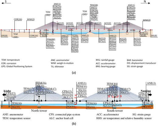
Large numbers of sensors were installed on the two bridges, including thermal sensors, corrosion sensors, Global Positioning System (GPS), connected pipe system (CPS), anemometers, weigh-in-motion systems and so on. A total of 2184 sensors are installed on the QC, while a total of 1078 sensors were applied to the NDB. The specific sensor placement on the two bridges is shown in Figure 1. The locations of the applied sensors are quite similar between the two bridges. The sensors mainly focus on critical positions from the mechanical perspective, including towers, mid-span area, quarter span area and the longest stay-cable sections.
To compare the SHM systems of the two bridges in a general way, Table 1 lists the statistical results of the applied sensors. Since the QC is relatively newly built, some advanced sensors are used, such as corrosion sensors and bearing gauges. Temperature, wind, vehicles (weights and numbers), acceleration, deflection, tilt and strain are monitored on both bridges, as is normal in bridge SHM systems. Compared with the NDB, the QC monitors additional parameters: the barometric pressure, rainfall, displacement, bearing pressure and corrosion. The NDB measures cable forces by using anchor load cells, while the QC has no transducers on stay cables to measure cable forces.
3. Digital twin analytic
Due to the limitations of budgets, it is impossible to monitor all structural sections when designing an SHM system. In this regard, critical sections need to be determined to maximise the SHM efficiency. At the design stage, the sections with the maximum moments are always selected as the critical sections to control the design. Thus, it is recommended to determine the monitored sections for SHM design as those with the maximum moments under designed loads.
3.1 Possible monitored sections for the QC
A finite-element model of the QC was built and updated by using Midas software, where 1793 nodes and 1405 elements are applied. The Eurocode EN 1993-1-11 (BSI, 2006) is used for the design work. In the Eurocode, there are four vehicle load models. Through the calculation and discussion, the load model I (i.e., the tandem system + uniformly distributed load) is the controllable load model.
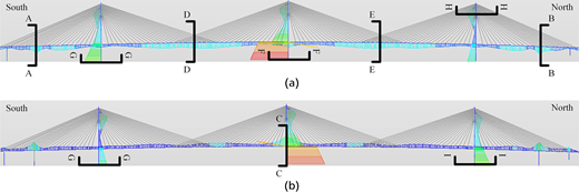
Under the load model I, the sagging and hogging moments are plotted in Figure 2. For girder sections, the south and north auxiliary pier sections (i.e., sections A–A and B–B) bear the maximum sagging moments, while the centre tower section (i.e., Section C–C) bears the maximum hogging moment. In addition, the sagging moments at the south and north mid-span are the secondary maximum values, termed as sections D–D and E–E. For tower sections, the centre tower bottom section bears the maximum sagging and hogging moments, and is termed as section F–F. Generally, moments in the south and north towers are relatively smaller than those of the centre tower. For the south tower, the bottom section (i.e., section G–G) bears the maximum sagging and hogging moments, while for the north tower, the maximum sagging moment is at the upper tower section (i.e., section H–H) and the maximum hogging moment is at the bottom (i.e., section I–I).
3.2 Possible monitored sections for the NDB
A finite-element model of the NDB was built and updated by using Midas software, including 5515 nodes and 3805 elements. The Chinese highway design code JTG/T D65-01-2007 (MoT, 2007) is employed to design the bridge.
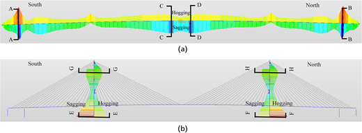
Under the Chinese designed load model, the sagging and hogging moments are plotted in Figure 3. For girder sections, the south and north auxiliary pier sections (i.e., sections A–A and B–B) bear the maximum sagging and hogging moments. In addition, the sagging moments near the mid-span are the secondary maximum values, termed as sections C–C and D–D. For tower sections, the bottom sections (i.e., sections E–E and F–F) bear the maximum sagging and hogging moments. The secondary maximum sagging and hogging moments are at the upper tower section (i.e., sections G–G and H–H).
The aforementioned possible monitored sections are critical sections from the perspective of mechanical analysis. However, the finally determined monitored sections should consider practical situations, such as the difficulty of sensor installation and the service environment of sensors.
4. SHM data analysis using a digital twin
In this study, the concept of using a digital twin is discussed to inform the planning of SHM system design in the future.
First, the data storage strategies for the two bridge SHM systems are analysed. In the QC SHM system, all the data are stored with a resampling frequency of 1 Hz even though the original sensor frequency may be higher (e.g., 10 Hz). This lower initial monitoring frequency was chosen to save storage space and cost. However, under certain unusual conditions (e.g., storms/typhoon), measurements in this time window will be stored with their original maximum frequency for further data mining.
In the NDB SHM system, all the data are recorded and stored with the original higher sampling rate, where most of the sensor frequencies are 10 Hz. Thus, more storage space is required by using the NDB system when compared with the QC system.
The QC system will keep original records of anomalous events and keep records using a frequency of 1 Hz in the normal operational time. However, 1 Hz sampling data is sometimes not sufficient for certain analysis – for example, dynamic analysis. For instance, 1 Hz acceleration data are inadequate to calculate structural frequencies or modal shapes under the ambient excitation. It is a trade-off to decide the sampling frequency by taking storage space and feasibility of further data mining into account. If all the data are stored with a high frequency, it will require more storage space. If all the data are stored with a relatively low frequency, some data mining methods will fail.
4.1 Temperature data
Temperature is a major load for large-scale bridges, leading to secondary stresses. Considering the importance of temperature loads, thermal sensors are often installed on bridges to monitor ambient temperatures and structural temperatures. In addition to the ambient temperature, the structural temperature is the load of interest to generate secondary stresses directly. For cable-stayed bridges, the temperature field on the girder, tower and cable is one of the most critical factors to influence the force distribution. In this regard, temperature data measured from the three components are discussed in the following section.
4.1.1 Temperature data on the girder section
For cable-stayed bridges, two types of structural temperatures are dominant factors for thermal effects: uniform temperature and temperature difference. Many thermal sensors are installed on girder sections to measure temperature fields. For instance, both bridges have sensors on the girder section to measure temperature data. The uniform girder temperature is used to determine the maximum displacement of girder ends, which is used to determine the types of expansion joints and bearings. Temperature difference of the girder section can also be influenced by solar radiation. Based on previous studies, temperature difference of the girder section is a main load to generate thermal effects (Xu et al., 2019c; Zhou and Sun, 2019a).
4.1.1.1 Thermal effects of localised elements
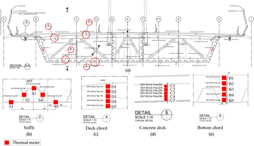
The placement of thermal sensors on the girder section of the QC is shown in Figure 4, whose sampling rate is 1 Hz. Five thermal sensors are installed around the girder soffit as shown in Figure 4(b) to monitor temperature distribution of the girder soffit. One year’s data (July 2020–June 2021) from the five thermal sensors are used for discussion. Measurements in January and April 2021 are missing since the SHM system was still under evaluation. Then, temperature differences between each pair of sensors were calculated, and the maxima of these temperature differences are calculated. The maximum temperature difference of the soffit is around 2.5°C in one year. The distribution of the temperature difference is shown in Figure 5(a). The temperature difference of the soffit is mainly distributed between 0 and 2.0°C. The relatively small temperature difference on the girder soffit results from the rare contact with solar radiation.
Five thermal sensors are installed on the deck chord along the vertical direction as shown in in Figure 4(c). Temperature measurements in one year (July 2020–June 2021) are used for discussion. The maximum value of the temperature differences is calculated. The distribution of temperature differences is shown in Figure 5(b). The temperature difference is mainly distributed from 0°C to 0.8°C. The extremely small temperature difference of the deck chord is due to its small thickness and the high thermal conductivity of steel materials.
Five thermal sensors are installed on the concrete deck along the vertical direction as shown in Figure 4(d). The maximum value of the temperature differences is calculated. The distribution of temperature differences is shown in Figure 5(c). The temperature difference of the concrete deck is mainly distributed from 0°C to 6°C. A relatively large temperature difference is observed owing to the large thickness of the concrete deck and its low thermal conductivity.
Five thermal sensors are installed on the bottom chord along the vertical direction as shown in Figure 4(e). The maximum value of the temperature differences is calculated. The distribution of temperature differences is shown in Figure 5(d). The temperature difference of the bottom chord is mainly distributed from 0°C to 1.5°C. A relatively small temperature difference on the deck bottom chord is seen since direct solar radiation has little influence on the bottom chord.
4.1.1.2 Thermal effects of main elements
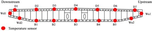
When compared with the thermal sensors installed on the girder section of the QC, a relatively small number of thermal sensors are installed on the NDB girder section (Figure 6), where the temperature sensor records temperature readings each half an hour. Seven thermal sensors along the transverse direction are used to measure deck chord temperatures, four are used to measure web temperatures and five are used to measure girder bottom chord temperatures.
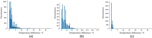
Temperature measurements on the NDB in 2007 from the deck chord are taken into account. The maximum temperature differences are calculated. The maximum value is around 30°C. Since outliers and zeros in the temperature measurements are not detected and deleted in the raw data, the single high temperature difference may result from outliers. In this regard, the temperature difference of the deck chord could refer to the distribution – Figure 7(a). The temperature difference of the transversal deck chord is mainly distributed from 0°C to 10°C. The large temperature difference of the transversal deck chord results from the large scale of the steel box girder: six running lanes wide compared with four lanes on the QC.
The maximum temperature differences within webs are calculated. The distribution of temperature differences is shown in Figure 7(b), which is between 0 and 5°C. A large temperature difference is observed due to the different solar radiation intensity between the two side webs. For the web directly receiving solar radiation, its temperature will rise rapidly, and vice versa.
The maximum temperature differences within the bottom chord are calculated. The distribution of temperature differences is shown in Figure 7(c), which is between 0 and 2°C. A relatively small temperature difference is seen along the transverse bottom chord since only rarely would solar radiation reach the bottom chord.
4.1.2 Temperature data on the tower section
The temperature distribution on the tower section is a critical factor to structural thermal response analysis. Thermal sensors are always used to measure temperature fields on tower sections.
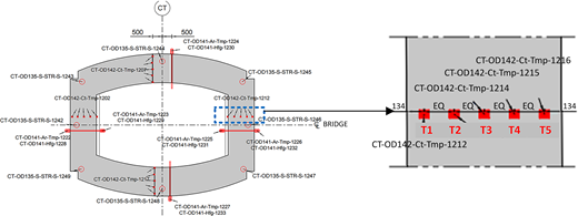
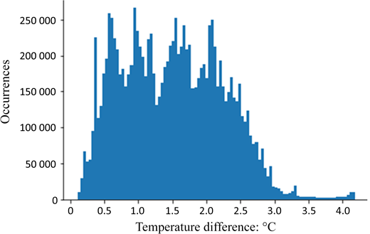
The sensor placement on the QC tower section is shown in Figure 8. Five thermal sensors are installed within the body of the tower shell, running along the thickness from the inner surface to the outer surface, to measure the temperature distribution. The issue of missing data is more serious in tower temperature data than in girder temperature data. The maximum temperature difference is calculated. The distribution of the temperature difference is shown in Figure 9, which is between 0 and 5°C. The relatively large temperature difference along the thickness of the tower shell results from the thickness of the tower shell and its low thermal conductivity. The temperature measured by the thermal sensor near the outer tower shell is largely affected by ambient temperatures and solar radiation, where significant oscillation is observed.
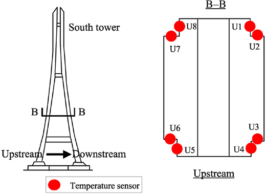
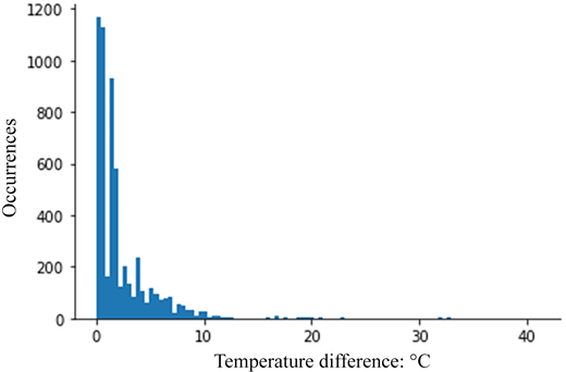
The thermal sensor placement for the NDB tower section is shown in Figure 10. Eight sensors are installed on one single tower leg section. The maxima of the temperature differences are calculated, and their distribution is shown in Figure 11. The temperature difference is distributed from 0°C to 10°C. The large temperature difference is observed due to different intensity of solar radiation for the measured locations.
4.1.3 Temperature data on the cable section
The NDB has no thermal sensors inside the stay cables, while thermal sensors are installed inside stay cables of the QC to measure their temperatures.
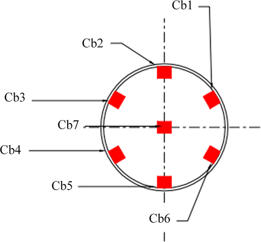
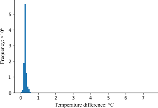
The sensor placement inside QC stay cables is shown in Figure 12. Six sensors are installed on the internal surface of cables, and one is installed at the centre of the cable section. The maxima of the temperature difference are calculated. The distribution of the temperature difference is shown in Figure 13, which is from 0°C to 0.5°C. The extremely small temperature difference is observed even though one thermal sensor is installed at the centre of the cable section. The relatively small temperature difference within the cable section results from the small scale of cables and large thermal conductivity of steel material.
4.2 Wind data
Wind load is another major external load for bridges. Anemometers are installed to measure site-specific wind features, including wind speed, wind direction and so on.
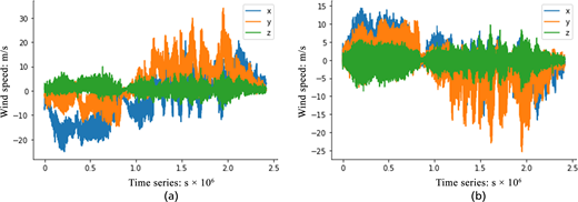
In the QC SHM system, anemometers, whose sampling rate is 1 Hz, are installed at the tower top level and deck level. One month of wind speed components in three directions are plotted in Figure 14. Different patterns of wind speeds are seen, where wind speeds at the tower top level are relatively larger than those at the deck level.
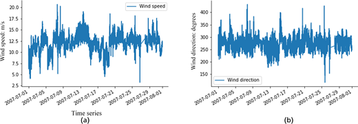
In the NDB SHM system, two ultrasonic anemometers with a sampling frequency of 10 Hz are used to measure deck-level wind features, and no anemometer is used to monitor wind features at the tower top level. The measured wind speed and direction at the deck level are shown in Figure 15. Since the NDB is located inland, the wind speed is relatively small when compared to bridges on the coast or in tidal estuaries.
4.3 Deflection data
Girder deflection is a critical global factor to indicate service condition of bridges. Normally, the girder deflection, especially at mid-span and quarter span, is monitored. In the QC system, the deflection is measured by GPS with a sampling rate of 1 Hz, while in the NDB system, the deflection is monitored by the CPS with a frequency of 10 Hz.
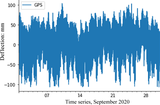
The south mid-span girder deflection measurements of the QC in September 2020 are shown in Figure 16. The variation range of the girder deflection is between −100 mm and +100 mm. The slow variation trend is caused by the temperature change.
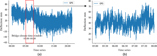
Due to ice falling from the tower and stay cables, the QC was closed on 4 December 2020 to ensure the safety of drivers. The GPS measurements during the bridge closure time window are shown in Figure 17. Although no vehicles were on the main bridge of the QC due to the bridge closure, the variation range of GPS measurements is still at a large level, varying between 10 mm and 70 mm.
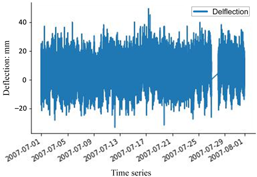
The CPS is used to monitor girder deflections for the NDB. The mid-span girder deflection measurements in July 2007 are shown in Figure 18. The deflection in July varies between −20 mm and +40 mm.
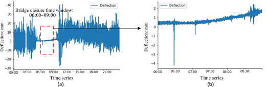
Due to heavy fog, the NDB was closed on 25 March 2007. The measured deflection data during the bridge closure time window are shown in Figure 19. An extreme narrow signal oscillation in the bridge closure time window is observed when compared with other normal operational conditions.
Although the main spans of the two bridges are very similar to each other, the mid-span deflection range variation is significantly different. The difference between the varying ranges of the two bridges – that is, 200 mm for the QC and 60 mm for the NDB – results from the discrepancy of vehicle loads and structural stiffness of the two bridges.
The significantly different signal patterns of the GPS and CPS data in the bridge closure time windows are caused by measuring errors of the two sensor types. To be specific, the measuring error of GPS in the vertical direction (i.e., z-direction) is 10 mm, which is a large magnitude considering the deflection variation range is only around 200 mm; using differential GPS, this can be reduced to 2 mm. The measuring error of the CPS, however, is 0.5 mm, a level of accuracy that is adequate for deflection measurements.
4.4 Discussion
Data from thermal sensors, anemometers and deflection sensors (i.e., GPS and CPS) are discussed in this study. According to the aforementioned data features, the sensor placement, sampling frequency and sensor type selection are analysed in this section.
A large number of thermal sensors are installed on the QC. The large temperature data set is a solid foundation for thermal field analysis. However, based on these measured data, some sensor placement advice could be proposed to guide SHM system design in other bridges. Many temperature differences of components are monitored in the QC system. The temperature differences of the girder soffit, deck chord, girder bottom chord and cable section are minor. Thus, this full-scale experiment indicates that it will not be strongly recommended to install five or more thermal sensors to measure temperature distributions of these components on future bridges. Instead, it is advised to install one or two sensors on these components. In detail, for those sensors that are easily replaced, one thermal sensor is recommended. For those sensors that are not easily replaced, two or more thermal sensors are recommended. The extra sensor is a back-up in case of the failure of one of the sensors. The determination of the number of redundant sensors should be based on the budget. More redundancy requires more economic investment, while less redundancy results in missing data after sensor failure.
For the concrete deck and tower shell, large temperature differences are observed. It is advised to install five or more thermal sensors in these sections to measure temperature distributions.
Since the temperature is a factor that varies slowly over time, it is not necessary to obtain temperature data at a high frequency. In addition, measured temperatures are always used to analyse temperature distributions of structural components or to establish relationships between temperatures and structural responses, which are not sensitive to the sampling frequency (Ding et al., 2012; Zhou and Sun, 2019b). Based on previous data mining experience associated with temperature data, 10 min acquiring a datum is adequate for any further data mining (Xu et al., 2021a, 2021b; Yue et al., 2021).
Based on data obtained from anemometers of the QC, different patterns of wind feature at the tower top and deck levels are observed. In general, wind speeds at the tower top level are stronger than those at the deck level. It is advised to install anemometers at tower top and deck levels to capture different wind patterns. It may be worthwhile to install wind sensors at intermediate levels to check whether these is a linear correlation with height. Wind features are always used to interpret the dynamic response (e.g., buffeting response) for bridges, which requires a relatively high sampling rate (Wang et al., 2013, 2019). The frequency of anemometers is recommended to be 10 Hz or higher to satisfy the requirement of further dynamic analysis.
Both GPS and CPS are sufficient to measure girder deflections in practice. According to the deflection data from the QC and the NDB, the CPS has a higher measuring accuracy than GPS. Since the GPS is easily replaced, for those bridges with large deflection amplitude, GPS is recommended. For those bridges with relatively small deflection amplitude, CPS is recommended. Since deflection data is a global index, it will not oscillate rapidly over time. In addition, deflection data are always used for static analysis, which does not require a high sampling frequency (Xu et al., 2020; Zhou et al., 2020). For the girder deflection measurement, a frequency of not lower than 1 Hz is advised.
5. Practical aspects of locating sensors
In this study, sensor location choice using digital twins is conducted based on the case studies of two cable stayed bridges: the QC and the NDB. A digital twin – that is, a simulated numerical model – is used to determine possible critical sections for monitoring from the mechanical perspective. Critical sections of towers and girders associated with the maximum sagging and hogging moments are decided upon according to the digital twin calculation results. However, the finally determined monitored sections should consider practical situations, such as the difficulty of sensor installation and the service environment of sensors.
Three types of sensors are discussed based on their measurements: these are thermal sensors, anemometers and deflection sensors. Advice regarding monitored sections, sensor placement, sampling frequency and sensor type selection are presented based on actual measurements from the two bridges. For thermal sensors, components with low temperature differences (e.g., girder soffit, deck chord, girder bottom chord and cable section) are not strongly recommended due to their small temperature difference magnitudes. In contrast, components with high temperature differences – for example, the concrete deck and the tower section – are advised to be measured by installing five or more sensors. A frequency of 1/600 Hz (i.e., 10 min obtaining one datum) is adequate for temperature sensors. The tower top level and deck level have quite different wind feature patterns, and anemometers are recommended to capture wind features at these two levels. A 10 Hz sampling rate for the anemometer satisfies the requirement of further research. GPS is recommended for those bridges with large deflection amplitude; for those with relatively small deflection amplitude, CPS is recommended. The sampling frequency of deflection sensors is advised to be higher than 1 Hz.
6. Conclusions
The conclusions are drawn as follows.
Possible monitored sections of the towers and girders are determined based on mechanical analysis through finite-element models.
For thermal sensors, monitoring of temperature differences of the girder soffit, deck chord, girder bottom chord and cable section are less strongly recommended due to their small temperature difference magnitudes. Temperature difference measurements of the concrete deck and tower section are advised, by installing five or more sensors. The sampling rate for thermal sensors is recommended to be 1/600 Hz (i.e., 10 min obtaining one datum).
Two critical locations are advised to install anemometers – the tower top level and deck level – since they have quite different wind feature patterns. A 10 Hz sampling rate is recommended for the anemometers in order to satisfy the requirement of future research.
For those bridges with large deflection amplitude, GPS is recommended, whilst for those with relatively small deflection amplitude, CPS is recommended. The sampling frequency of deflection sensors is advised to be higher than 1 Hz.