


The primary aim of this paper is to examine the role of asymmetry in the relationship between FDI shocks and real GDP across seven selected Asian countries, contributing to a deeper understanding of how FDI influences economic growth in the region.
This study employs two advanced methodologies: the nonlinear autoregressive distributed lag (NARDL) model and the generalized impulse response function (GIRF). The NARDL model is used to explore both the long- and short-term asymmetric effects of FDI on real GDP, while the GIRF is employed to analyze the responses of GDP to both positive and negative FDI shocks.
The results reveal that FDI asymmetrically affects real GDP in the long run in five of the countries under consideration: Indonesia, Malaysia, the Philippines, Singapore and Thailand. Short-term asymmetry is also confirmed for Malaysia, Thailand and Japan. Additionally, the GIRF analysis demonstrates that the responses of GDP to positive and negative FDI shocks differ significantly and are not mirror images.
The findings have important policy implications, suggesting that policymakers should consider the asymmetrical effects of FDI when designing economic strategies and responses to foreign investment shocks. These insights can enhance empirical modeling and contribute to more effective economic planning in the region.
This paper is unique in its explicit focus on asymmetry in the relationship between FDI shocks and real GDP, applying advanced econometric techniques to provide a more nuanced understanding of this dynamic. The study’s results offer valuable contributions to both policy analysis and empirical modeling in the context of Asian economies.
1. Introduction
Foreign Direct Investment (FDI) is widely regarded as a critical driver of economic development in host countries. It provides not only capital inflows but also essential channels for technology transfer, management expertise, productivity enhancement, and integration into global markets. Among various forms of external financing, FDI is considered the most stable and less volatile during periods of global financial crisis, making it highly valued, especially for emerging economies.
Despite these theoretical benefits, the empirical evidence on the FDI-growth relationship is mixed. Several studies affirm a positive contribution of FDI to economic growth across diverse country settings (Sijabat, 2023; Yusuf et al., 2020; Okwu et al., 2020; Sengupta and Roma, 2020; Agyapong and Kojo, 2020; Akadiri et al., 2019). They emphasize the role of FDI in fostering knowledge spillovers, upgrading technology, and stimulating capital accumulation. Conversely, several empirical investigations reveal negative impacts of FDI on growth (Sothan, 2017; Rehman, 2016). Critics argue that under certain conditions, FDI can crowd out domestic investment, perpetuate dependency, distort market structures, and exacerbate income inequalities. Some studies even document the “race to the bottom” phenomenon, where host countries relax environmental and labor standards to attract foreign investors. Additionally, a third strand of the literature finds no statistically significant relationship between FDI and GDP growth, suggesting a neutrality hypothesis (Magazzino and Mele, 2022; Kathuria, 2019; Phuong and Tuyen, 2018). These findings indicate that the FDI-growth nexus is not universally positive, and its direction and magnitude may depend on various structural and institutional factors within the host economy.
Recognizing the FDI-growth relationship, scholars have increasingly emphasized that the impact of FDI may be contingent on country-specific absorptive capacities, such as human capital development, financial system maturity, technological capabilities, and institutional quality (Joo et al., 2022; Carbonell and Richard, 2018). Consequently, FDI’s contribution to sustainable economic growth cannot be assumed to be homogeneous across countries or over time. Moreover, the dynamic response of economic growth to FDI shocks may not be symmetric. Traditional linear models typically assume that positive and negative FDI shocks exert identical effects, merely differing in direction. However, real-world economic dynamics often exhibit asymmetries, particularly in the presence of structural rigidities, institutional constraints, and behavioral adjustments (Shin et al., 2014). Ignoring potential asymmetries could lead to misinterpretation of FDI’s real economic effects and, consequently, to flawed policy recommendations.
Against this backdrop, this study addresses an important gap in the literature by focusing on the nonlinear and asymmetric effects of FDI on sustainable GDP growth across seven selected Asian economies: Indonesia, Malaysia, Philippines, Singapore, Thailand, South Korea, and Japan. Thus, the primary objective of this research is to investigate whether positive and negative FDI shocks have asymmetric impacts on economic growth in both the short and long term, thereby offering more accurate insights for policy design.
The focus on Asia is especially relevant given recent FDI dynamics in the region. According to the Asia-Pacific Trade and Investment Trends Report (2021, 2022) and the World Investment Report (2022a, b), FDI inflows to Asia declined sharply during the COVID-19 pandemic. For instance, Indonesia experienced an FDI reduction of approximately $5 billion. Malaysia saw a decline of 54%. The Philippines suffered a 21.33% fall. Thailand witnessed a dramatic 247% contraction. South Korea and Japan also reported declines of 9 and 30% respectively. Although signs of recovery emerged by 2021 and 2022 (ASEAN Investment Report, 2022; UNCTAD, 2021), the fluctuations in FDI inflows highlighted the vulnerability of Asian economies to external shocks, reinforcing the need to understand how FDI shocks—positive and negative—affect sustainable GDP growth differently.
Moreover, the strategic importance of FDI for Asia’s development cannot be overstated. According to the ASEAN Investment Report (2022), the region’s share of global FDI inflows increased from 11% in 2018–2019 to 12% in 2020–2021. Asian economies have diversified beyond traditional manufacturing into sectors such as digital economy, green infrastructure, healthcare innovation, and renewable energy (World Investment Report, 2023). In 2023, FDI trends across the selected Asian economies displayed notable variation. Indonesia recorded a 4% increase in FDI inflows, reaching $22 billion. Malaysia experienced a significant rise of 39%, achieving a record $17 billion, driven largely by investments in manufacturing and greenfield projects. In contrast, the Philippines saw a 23% decline in FDI inflows, influenced by domestic acquisitions of foreign affiliates. Singapore maintained its position as a regional hub, attracting a record $141 billion in FDI and accounting for nearly two-thirds of ASEAN’s total inflows. FDI data for Thailand in 2023 was not specifically detailed in the available sources. South Korea experienced an 18% decrease in FDI inflows, totaling $18 billion. Meanwhile, Japan reached its highest-ever level of FDI inflows at $33 billion (World Investment Report, 2023).
Given this backdrop, the methodology adopted in this paper is designed to capture the nonlinear and asymmetric nature of the FDI-growth nexus. Specifically, our research employs the Nonlinear Autoregressive Distributed Lag (NARDL) model developed by Shin et al. (2014) and the Generalized Impulse Response Functions (GIRF) by Koop et al. (1996) and Pesaran and Shin (1998), which allow for disaggregation of FDI inflows into positive and negative shocks, distinction between short-run and long-run asymmetric impacts, and more realistic modeling of economic adjustment processes following FDI fluctuations. Positive FDI shocks may strengthen productivity and investment channels more efficiently when host countries exhibit strong absorptive capacity (e.g. high human capital, developed financial systems, strong institutional frameworks). Negative FDI shocks may exacerbate vulnerabilities in economies with weaker absorptive capacity, magnifying adverse impacts through channels like reduced investment, technology withdrawal, or employment losses.
To ensure robustness and comprehensiveness, we incorporate several control variables, notably capital formation, trade openness, and population growth. These variables have been widely recognized as important determinants of economic performance in the existing literature (Topcu et al., 2020; Onyinye et al., 2017; Cleeve et al., 2015; Hasli et al., 2015; Kim, 2016; Peterson, 2017). By controlling these factors, the study isolates the net effect of FDI shocks on sustainable GDP growth more accurately.
In sum, this paper aims to contribute to the existing literature by providing empirical evidence on the nonlinear and asymmetric responses of sustainable GDP growth to FDI shocks in selected Asian countries, using a rigorous econometric framework and comprehensive control mechanisms. This distinguishes the current from previous studies, which assessed whether FDI inflow may exert a positive or negative impact on economic growth in the host economy as well as other studies that explored the causal relationship between the trends of these two macro variables. Furthermore, we explicitly define sustainable GDP growth not merely in terms of short-term output increases, but as inclusive, resilient, and environmentally sound economic expansion. This broader conceptualization of growth aligns the analysis with contemporary policy priorities in the selected Asian economies.
Our findings indicate that FDI asymmetrically affects real GDP in the long run for five Asian economies: Indonesia, Malaysia, Philippines, Singapore, and Thailand. The short-run asymmetry is confirmed for Malaysia, Thailand, and Japan. When examining the GIRF, we found that the responses of these sample countries’ to the positive FDI shocks are significant in most countries. In contrast, the negative shock has a relatively minor impact on the GDP of these countries. Therefore, the GIRF analysis further affirms the presence of an asymmetric effect of shocks on across the sampled Asian countries. Additionally, the findings are expected to offer valuable insights for policymakers seeking to design targeted strategies to maximize the developmental benefits of FDI, especially in the context of post-pandemic recovery and long-term sustainable development ambitions.
2. Review of literature
Numerous studies have been conducted to thoroughly investigate the impact of FDI on economic growth through typically utilizing the neoclassical and endogenous economic growth models (Deonanan and Daren, 2022; An and Kuo-Chun, 2021; Udeogu et al., 2021; Hagan and Anthony, 2020). The neoclassical paradigm states that FDI influences economic growth by fostering capital accumulation, technology spillover, and enhancing the short-term efficiency of the host countries’ economies (Guvercin and Adem, 2021; Yusuf et al., 2020), while the endogenous model posits that economic growth is directly linked with FDI inflow (Bambi et al., 2017). Nevertheless, despite the impact of FDI inflow on GDP growth has been extensively examined in literature; however, the results remain inconclusive and exhibit varying results due to differences in the estimation methods employed, variations in the selected samples, in addition to disparities in the time periods across studies.
In this regard, various studies endorse the significant positive impact of FDI on economic growth based on the FDI spillover externalities on the host economy (i.e. Wang (2019) for the Asian countries; Akadiri et al. (2019) for twenty-five African countries; Elian et al. (2020) for the BRICS (Brazil, Russia, India, China, South Africa) countries; Cakerri et al., 2020, Agyapong and Kojo (2020) for Africa, Mowlaei and Intezar (2021) for a group of 30 Islamic countries) [1]. Nonetheless, certain studies have determined that the positive impact of FDI on growth is statistically insignificant (i.e. Yusuf et al. (2020) for West Africa, Shahzad et al. (2019) for Brazilian economy, Gunby et al. (2017) for China). A further set of studies revealed a negative growth effect of FDI, attributed to the crowding out of domestic investments and expanding external vulnerability (Sağlam, 2017; Rehman, 2016). A key strand of literature supports the conditional effect argument, suggesting that the effectiveness of FDI in stimulating economic growth is contingent on preexisting conditions within the host economy. These preconditions, referred to as specific features, act as absorptive capacities that enable the host economy to fully harness the benefits of FDI inflows (Joo et al., 2022; Ibhagui, 2020; Dinh et al., 2019; Carbonell and Richard, 2018) [2].
Current studies highlight the significant role of Foreign Direct Investment (FDI) in economic growth. Phan Le et al. (2024) show that a 1% increase in FDI boosts economic growth by 9.3% in middle-income countries, with total factor productivity playing a key role. Rodríguez-Chávez (2024) noted a 3% global increase in FDI, but a 9% decline in developing countries, with Asia most affected. The UNCTAD World Investment Report (2024) reports an 11% rise in global FDI to $1.4 trillion, mainly driven by European conduit economies. Recent international reports highlight a mixed global outlook. The International Monetary Fund (IMF, 2025) reports that global inward FDI rose by 4.4% in 2023, reaching approximately $41 trillion, supported by strong inflows to emerging economies. In parallel, the Organization for Economic Co-operation and Development (OECD, 2025) forecasts a slight deceleration in global GDP growth, from 3.2% in 2024 to 3.1% in 2025, attributed to rising trade barriers and heightened policy uncertainty. Kenh and Wei (2025) emphasize that FDI is most effective when directed toward sectors with a comparative advantage, significantly boosting economic development. Korsah et al. (2025) identify natural resources, market size, trade openness, and exchange rate strength as key determinants of FDI inflows into West African countries, noting that French-speaking nations attract more FDI than their English-speaking counterparts. Arya et al. (2025) confirm a long-term relationship between trade, FDI, and economic growth, with bidirectional causality between GDP and FDI in most countries, and exports contributing notably to GDP growth in several cases.
Our paper incorporates country-specific features such as the country’s capital formation, trade openness, and population growth rate, which have been identified as significant factors in previous studies examining the FDI-GDP growth nexus. Capital formation is commonly regarded as a beneficial factor for a country’s economic growth, as evidenced by existing literature indicating its positive impact on economic growth (i.e. Ntamwiza and Masengesho (2022), for Rwanda; Pasara et al. (2020), for South Africa; Awodumi and Adewuyi (2020), for Angola and Egypt; Muhammad and Khan (2019), for 35 Asian countries; Khan et al. (2019), for 193 countries; Erum and Hussain (2019), for 43 members of the Organization of Islamic Corporation (OIC) countries; Bal et al. (2016), for India); Trade openness is another vital characteristic of host country that has received substantial attention in the literature on the relationship between FDI and economic growth. Numerous studies have validated the significant role of trade openness in promoting economic growth (Cinar and Nulambeh, 2018; Khamphengvong and Srithilat, 2017). The population growth rate is an additional crucial host country feature that plays a role in the impact of FDI on economic growth. Kim (2016) conducted an estimation of how the fluctuating age configuration of the population has affected GDP growth, ultimately concluding that demographic changes would result in a significant downward trend in economic growth. Peterson (2017) found that the influence of population growth on economic growth is contingent on the income level of the country. In high-income countries, a high population growth rate is likely to alleviate the country’s social and economic challenges, while in low-income countries may impede economic development.
3. Data and model
3.1 Data collection
This study examines the asymmetric relationship between foreign direct investment (FDI) and real gross domestic product (GDP) in seven Asian economies: Indonesia, Malaysia, the Philippines, Singapore, Thailand, South Korea, and Japan [3]. The analysis utilizes annual data spanning the period 1970–2019. Table 1 provides the definitions of the variables employed, along with their respective data sources.
Description of data
| Variables | Data source | Scale unit |
|---|---|---|
| FDI, net inflows | World Development Indicators (WDI) | % of GDP |
| GDP per capita | World Development Indicators (WDI) | constant 2015 US$ |
| Gross capital formation | World Development Indicators (WDI) | % of GDP |
| Exports of goods and services | World Development Indicators (WDI) | % of GDP |
| Imports of goods and services | World Development Indicators (WDI) | % of GDP |
| Population growth | World Development Indicators (WDI) | annual % |
3.2 Model specification
In conceptualizing the long-run impact of foreign direct investment (FDI) on real gross domestic product (GDP), this study follows the recent strand of literature and adopts the following long-run specification:
where is real GDP (base year is 2015), is net inflows of foreign direct investment (% of GDP), is gross capital formation (% of GDP), is trade openness as exports plus imports of goods and services (% of GDP), is population growth (annual %), and is the standard error term (see appendix 1). All variables are measured in logarithms.
In Equation (1), to denote the long-run effects of the explanatory variables—namely (, , , ) on . As demonstrated by Pesaran et al. (2001), Equation (1) can be estimated within the framework of an Error Correction Model (ECM). A major advantage of the ECM approach is that it enables the simultaneous estimation of both short-run dynamics and long-run relationships within a single equation. The ECM specification is expressed as follows:
According to Pesaran et al. (2001), Equation (2) identifies the short-run effects through the coefficients of the first-differenced variables (e.g. ), while the long-run effects are captured by the estimates of to normalized on (; ; ; ). This specification, developed by Pesaran et al. (2001), is commonly referred to as the linear autoregressive distributed lag (ARDL) model.
The specification in Equation (1) implies that the explanatory variables (, , , ) affect real in a symmetric, or linear, manner. Symmetry in this context indicates that increases and decreases in an explanatory variable exert effects of equal magnitude but opposite direction on . However, Neftçi (1984) and Falk (1986) demonstrate that many macroeconomic variables exhibit nonlinear, or asymmetric, behavior over time. This suggests that fluctuations in may respond differently to increases versus decreases in the explanatory variables, both in magnitude and direction, thereby reflecting the concept of asymmetric effects.
To capture such dynamics, Shin et al. (2014) extended the linear ARDL framework to the nonlinear autoregressive distributed lag (NARDL) model, which allows for the identification of asymmetric effects [4]. We build on this framework by integrating Generalized Impulse Response Functions (GIRF), which provides a dynamic perspective on how GDP responds to asymmetric investment shocks over time.
The NARDL approach decomposes each explanatory variable (, , , ) into partial sums of positive (increasing) and negative (decreasing) changes. For instance, can be expressed as the cumulative sum of its positive and negative variations as follows:
and
where .
Similarly, is decomposed into and , into and , and into and . Constructing these partial sum variables enables the nonlinear adjustment of variations in the explanatory variables. Accordingly, Equation (1) can be reformulated within an asymmetric long-run framework as follows:
To estimate both the asymmetric short-run and long-run effects, the error correction model (ECM) is reformulated as follows:
Shin et al. (2014), building on the framework of Pesaran et al. (2001), demonstrate that in Equation (6) the asymmetric short-run effects are reflected in the estimated coefficients of the first-differenced variables (e.g. ), while the asymmetric long-run effects are captured by the coefficients to , normalized on (; ; ; ; ; ; ; ).
Shin et al. (2014) suggest that, once Equation (6) is estimated using the conventional Ordinary Least Squares (OLS) method, the presence of asymmetric effects of each explanatory variable on real can be formally assessed through Wald tests, provided that both the positive (+) and negative (−) partial sum components are statistically significant. For instance, the null hypothesis implies no long-run asymmetry, while the alternative indicates the existence of long-run asymmetry between real and variations in . Similarly, the rejection of the null hypotheses , , and would provide evidence of long-run asymmetry in the relationships between real and gross capital formation, trade openness, and population growth, respectively. In addition, short-run asymmetries are investigated through the coefficients of the first-differenced variables in Equation (6). For example, under the Wald test, the null hypothesis implies no short-run asymmetry, whereas the alternative indicates the presence of short-run asymmetry between real and fluctuations. Likewise, evidence of short-run asymmetry would arise if the hypotheses , , or are rejected, implying asymmetric short-run effects of gross capital formation, trade openness, and population growth, respectively.
The validity of NARDL inferences critically depends on the existence of cointegration, that is, a long-run equilibrium relationship among the variables. Accordingly, we test whether the variables in Equation (6) are cointegrated using the procedures of Pesaran et al. (2001) and Banerjee et al. (1998), which rely on the F-statistic and the -statistic, respectively. Under the Pesaran et al. (2001) bounds testing framework, evidence of cointegration is obtained when . By contrast, the null hypothesis of no cointegration is defined as [5]. In the Banerjee et al. (1998) test, cointegration is confirmed when (no cointegration if ). Establishing cointegration is therefore a necessary precondition; only once this is confirmed can the estimated NARDL model yield valid inferences regarding both the long-run and short-run asymmetric relationships.
Along with the NARDL model, this paper employs the generalized impulse response function (GIRF) as a second practice to examine the dynamic response of to the increase and decrease of across the seven Asian countries. To do so, we assume that is determined by hikes (positive shock), and falls (negative shock):
At this point, represents a shock in the kth variable, where k is the positive and negative shocks. GIRF is next uncovered through estimating Eq. (7). Accordingly, GIRF offers the responses of to a shock of one standard deviation in for the seven Asian countries.
4. Empirical findings
4.1 Inferences of the NARDL model: (a)symmetric effects of FDI on GDP
We start with a visual assessment of the time path of and variables to verify their co-movement. Figure 1 noticeably implies a kind of co-movement among the two variables, signaling the probability of a long-run association. Nevertheless, we need to properly analyze the presence of the long-run association (cointegration) as illustrated earlier.
 The figure 14 line graphs, arranged in seven rows and two columns. Each pair of line graphs is labeled for a specific country. For each country, the left graph is labeled “F D I” and the right graph is labeled “G D P.” The horizontal axis of all graphs ranges from 1970 to 2015, in increments of 5 years. The details of the graphs are as follows: The graphs in the first row are for “Indonesia.” The vertical axis for “F D I” ranges from negative 4 to 6 in increments of 2. The graph for “F D I” on the left starts at (1970, 1.8), shows fluctuations, and drops to (2000, negative 2.54), increases to (2005, 3.12), and fluctuates and ends at (2019, 2.41). The vertical axis for “G D P” ranges from 2.8 to 3.6 in increments of 0.2. The graph for “G D P” starts at (1970, 2.85), increases to (1997, 3.33), drops slightly and again rises to end at (2019, 3.6). The graphs in the second row are for “Malaysia.” The vertical axis for “F D I” ranges from 0 to 10 in increments of 2. The graph for “F D I” on the left starts at (1970, 2.67), fluctuates, reaches a peak at (1992, 8.8), declines to (2001, 0.80), then shows fluctuations, and ends at (2019, 2.67). The vertical axis for “G D P” ranges from 3.2 to 4.4 in increments of 0.2. The graph for “G D P” starts at (1970, 3.27), increases with small fluctuations to (1997, 3.82), continues upward, and ends at (2019, 4.07). The graphs in the third row are for “Philippines.” The vertical axis for “F D I” ranges from negative 1 to 4 in increments of 1. The graph for “F D I” on the left starts at (1970, 0.20), fluctuates, rises to (1997, 3.28), drops to (2004, 0.71), rises and ends at (2019, 2.12). The vertical axis for “G D P” ranges from 3.1 to 3.6 in increments of 0.1. The graph for “G D P” starts at (1970, 3.16), rises slowly, fluctuates around (1997, 3.27), then increases sharply and ends at (2019, 3.56). The graphs in the fourth row are for “Singapore.” The vertical axis of “F D I” ranges from 0 to 30 in increments of 5. The graph for “F D I” on the left starts at (1970, 5.3), fluctuates with sharp increases, reaches (1999, 22.1), dips, rises, and ends at (2019, 28.4). The vertical axis for “G D P” ranges from 3.8 to 4.8 in increments of 0.2. The graph for “G D P” on the right starts at (1970, 3.85), shows a steady increase, reaching (1997, 4.53), and ends at (2019, 4.80). The graphs in the fifth row are for “Thailand.” The vertical axis of “F D I” ranges from 0 to 7 in increments of 1. The graph for “F D I” on the left starts at (1970, 0.66), fluctuates with distinct peaks at (1998, 6.46), drops, and ends with fluctuations at (2019, 0.85). The vertical axis for “G D P” ranges from 2.8 to 4.0 in increments of 0.2. The graph for “G D P” on the right starts at (1970, 3), rises steadily to (1996, 3.57), increases more gradually, and ends at (2019, 4.83). The graphs in the sixth row are for “S. Korea.” The vertical axis of “F D I” ranges from 0 to 5 in increments of 1. The graph for “F D I” on the left starts at (1970, 0.77), rises sharply to (1972, 4.62), drops steeply and fluctuates below 1 after 1975, peaks at (1999, 2.18), and ends at (2019, 0.75). The vertical axis for “G D P” ranges from 3.2 to 4.8 in increments of 0.4. The graph for “G D P” on the right starts at (1970, 3.34), increases consistently to (1997, 4.2), and ends at (2019, 4.54). The graphs in the seventh row are for “Japan.” The vertical axis of “F D I” ranges from negative 0.2 to 1 in increments of 0.2. The graph for “F D I” on the left starts at (1970, 0.06), remains near zero, increases after 1995, reaching (2007, 0.5), rises with fluctuations and ends at (2019, 0.75). The vertical axis for “G D P” ranges from 4.1 to 4.6 in increments of 0.1. The graph for “G D P” on the right starts at (1970, 4.16), rises steadily to (2006, 4.52), fluctuates and ends at (2019, 4.57). Note: All numerical values are approximated.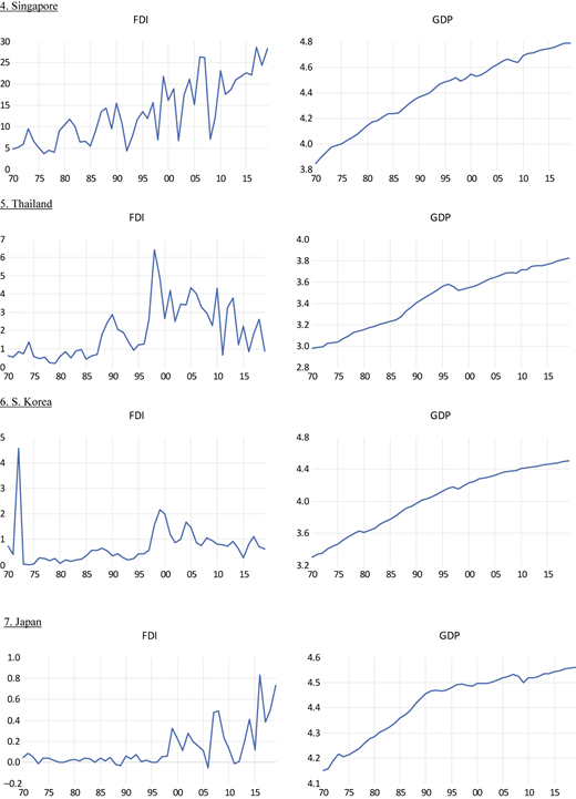
Time path movement of FDI and GDP. Source(s): The authors
The figure 14 line graphs, arranged in seven rows and two columns. Each pair of line graphs is labeled for a specific country. For each country, the left graph is labeled “F D I” and the right graph is labeled “G D P.” The horizontal axis of all graphs ranges from 1970 to 2015, in increments of 5 years. The details of the graphs are as follows: The graphs in the first row are for “Indonesia.” The vertical axis for “F D I” ranges from negative 4 to 6 in increments of 2. The graph for “F D I” on the left starts at (1970, 1.8), shows fluctuations, and drops to (2000, negative 2.54), increases to (2005, 3.12), and fluctuates and ends at (2019, 2.41). The vertical axis for “G D P” ranges from 2.8 to 3.6 in increments of 0.2. The graph for “G D P” starts at (1970, 2.85), increases to (1997, 3.33), drops slightly and again rises to end at (2019, 3.6). The graphs in the second row are for “Malaysia.” The vertical axis for “F D I” ranges from 0 to 10 in increments of 2. The graph for “F D I” on the left starts at (1970, 2.67), fluctuates, reaches a peak at (1992, 8.8), declines to (2001, 0.80), then shows fluctuations, and ends at (2019, 2.67). The vertical axis for “G D P” ranges from 3.2 to 4.4 in increments of 0.2. The graph for “G D P” starts at (1970, 3.27), increases with small fluctuations to (1997, 3.82), continues upward, and ends at (2019, 4.07). The graphs in the third row are for “Philippines.” The vertical axis for “F D I” ranges from negative 1 to 4 in increments of 1. The graph for “F D I” on the left starts at (1970, 0.20), fluctuates, rises to (1997, 3.28), drops to (2004, 0.71), rises and ends at (2019, 2.12). The vertical axis for “G D P” ranges from 3.1 to 3.6 in increments of 0.1. The graph for “G D P” starts at (1970, 3.16), rises slowly, fluctuates around (1997, 3.27), then increases sharply and ends at (2019, 3.56). The graphs in the fourth row are for “Singapore.” The vertical axis of “F D I” ranges from 0 to 30 in increments of 5. The graph for “F D I” on the left starts at (1970, 5.3), fluctuates with sharp increases, reaches (1999, 22.1), dips, rises, and ends at (2019, 28.4). The vertical axis for “G D P” ranges from 3.8 to 4.8 in increments of 0.2. The graph for “G D P” on the right starts at (1970, 3.85), shows a steady increase, reaching (1997, 4.53), and ends at (2019, 4.80). The graphs in the fifth row are for “Thailand.” The vertical axis of “F D I” ranges from 0 to 7 in increments of 1. The graph for “F D I” on the left starts at (1970, 0.66), fluctuates with distinct peaks at (1998, 6.46), drops, and ends with fluctuations at (2019, 0.85). The vertical axis for “G D P” ranges from 2.8 to 4.0 in increments of 0.2. The graph for “G D P” on the right starts at (1970, 3), rises steadily to (1996, 3.57), increases more gradually, and ends at (2019, 4.83). The graphs in the sixth row are for “S. Korea.” The vertical axis of “F D I” ranges from 0 to 5 in increments of 1. The graph for “F D I” on the left starts at (1970, 0.77), rises sharply to (1972, 4.62), drops steeply and fluctuates below 1 after 1975, peaks at (1999, 2.18), and ends at (2019, 0.75). The vertical axis for “G D P” ranges from 3.2 to 4.8 in increments of 0.4. The graph for “G D P” on the right starts at (1970, 3.34), increases consistently to (1997, 4.2), and ends at (2019, 4.54). The graphs in the seventh row are for “Japan.” The vertical axis of “F D I” ranges from negative 0.2 to 1 in increments of 0.2. The graph for “F D I” on the left starts at (1970, 0.06), remains near zero, increases after 1995, reaching (2007, 0.5), rises with fluctuations and ends at (2019, 0.75). The vertical axis for “G D P” ranges from 4.1 to 4.6 in increments of 0.1. The graph for “G D P” on the right starts at (1970, 4.16), rises steadily to (2006, 4.52), fluctuates and ends at (2019, 4.57). Note: All numerical values are approximated.Time path movement of FDI and GDP. Source(s): The authors
Previous to applying the NARDL model, we begin by checking the stationarity of the respective variables to disclose their order of integration. Regardless of the fact that the NARDL can be utilized whether the variables are of order zero, or order one, or even a mix of both (I(0), I(1)), as described before, still including I(2) variable in the NARDL model presents the possibility of spurious inferences (Pesaran et al., 2001). As a result, the first needed step for applying the NARDL is to verify that none of the series is I(2). While there are various tests available to investigate the unit root, the modified Dickey-Fuller unit root test with single break was used for each variable with the results shown in Table 2. The test assumes a null of unit root (non-stationarity). The results of Table 2 provide compelling evidence that the respective variables are not integrated of order two (I(2)), which denotes the appropriateness of using the NARDL model as the fundamental requirement is met.
Modified Dickey-Fuller test with break
| Variable | Level | 1st difference |
|---|---|---|
| Indonesia | ||
| −9.59*** (0) | −11.80*** (0) | |
| −4.27 (0) | −10.37*** (0) | |
| −5.36*** (0) | −8.52*** (0) | |
| −4.22 (0) | −9.77*** (0) | |
| −4.39 (10) | −9.07*** (10) | |
| Malaysia | ||
| −3.63 (0) | −7.51*** (0) | |
| −4.66 (0) | −8.30*** (0) | |
| −4.93 (0) | −7.22*** (0) | |
| −2.32 (0) | −7.05*** (1) | |
| −3.90 (8) | −8.62*** (6) | |
| Philippines | ||
| −2.04 (1) | −9.78*** (8) | |
| −4.54 (0) | −9.27*** (0) | |
| −4.88 (1) | −6.16*** (1) | |
| −3.18 (0) | −7.16*** (0) | |
| −4.90 (10) | −6.54*** (6) | |
| Singapore | ||
| −3.13 (0) | −7.99*** (1) | |
| −6.75*** (0) | −10.01*** (0) | |
| −3.70 (0) | −9.46*** (0) | |
| −3.12 (0) | −7.69*** (0) | |
| −4.18 (0) | −7.49*** (0) | |
| Thailand | ||
| −3.93 (1) | −8.30*** (0) | |
| −5.15 (0) | −11.12*** (0) | |
| −4.60 (0) | −8.76*** (0) | |
| −2.39 (0) | −8.11*** (0) | |
| −3.84 (7) | −8.16*** (6) | |
| S. Korea | ||
| −1.91 (0) | −7.93*** (0) | |
| −8.64*** (2) | −13.47*** (0) | |
| −3.74 (0) | −10.72*** (1) | |
| −3.45 (0) | −6.90*** (0) | |
| −5.22 (0) | −8.40*** (0) | |
| Japan | ||
| −2.68 (0) | −7.26*** (0) | |
| −6.73*** (0) | −10.71*** (0) | |
| −3.36 (1) | −6.27*** (0) | |
| −4.82 (0) | −7.24*** (0) | |
| −8.49*** (0) | −30.48*** (0) | |
Note(s): is real GDP (base year is 2015), is net inflows of foreign direct investment, is gross capital formation, is trade openness as exports plus imports of goods and services, is population growth. All variables in logarithmic format. Null Hypothesis: series has unit roots. Lag length, reported in parentheses, is selected by SIC with maximum lags = 10. *** denotes significance at the 1% level
Ahead of applying the NARDL analysis, we need to check for two issues. Firstly, investigate if there is support for the nonlinearity in the relationship between the engaged variables. A proper practice to employ is the Brock, Dechert, and Scheinkman test (BDS test) of Broock et al. (1996) that is often used to explore the presence of nonlinearity in the model. The BDS test postulates a null hypothesis of linearity in opposition to an alternative of nonlinearity. Secondly, test if the data suffers from shocks or unanticipated events (structural breaks). Gregory et al. (1996) report that if the analysis does not consider the structural breaks, the cointegration conclusions might be deceptive, since such breaks might produce unstable cointegration relationship, provided that the NARDL procedure requires evidence of cointegration. Thus, the test of Bai and Perron (1998) is applied to detect the structural breaks in the data. This test enables us to determine up to five breaks in addition to detecting its dates [6]. If structural breaks are found, the NARDL model allows, within the error correction model, to use dummy variables for the breaks. The dummy variable equals one starting from the break date and afterward and equals zero before the break date (Pesaran et al., 2001). The results of BDS test and Bai-Perron examination are reported in Tables 3 and 4, respectively.
BDS test (Broock et al., 1996)
| Country | m = 2 | m = 3 | m = 4 | m = 5 | m = 6 | |
|---|---|---|---|---|---|---|
| Indonesia | 0.059*** | 0.117*** | 0.142*** | 0.156*** | 0.155*** | |
| 0.161*** | 0.266*** | 0.335*** | 0.375*** | 0.397*** | ||
| 0.098*** | 0.174*** | 0.209*** | 0.214*** | 0.216*** | ||
| 0.205*** | 0.347*** | 0.447*** | 0.516*** | 0.565*** | ||
| Malaysia | 0.055*** | 0.075*** | 0.086*** | 0.079** | 0.074** | |
| 0.124*** | 0.200*** | 0.235*** | 0.244*** | 0.235*** | ||
| 0.181*** | 0.314*** | 0.404*** | 0.461*** | 0.491*** | ||
| 0.172*** | 0.276*** | 0.336*** | 0.368*** | 0.377*** | ||
| Philippines | 0.068*** | 0.085*** | 0.071*** | 0.049** | 0.047** | |
| 0.103*** | 0.167*** | 0.198*** | 0.204*** | 0.202*** | ||
| 0.164*** | 0.272*** | 0.342*** | 0.386*** | 0.401*** | ||
| 0.187*** | 0.308*** | 0.388*** | 0.442*** | 0.481*** | ||
| Singapore | 0.060*** | 0.101*** | 0.111*** | 0.120*** | 0.120*** | |
| 0.123*** | 0.206*** | 0.262*** | 0.292*** | 0.302*** | ||
| 0.112*** | 0.193*** | 0.239*** | 0.252*** | 0.256*** | ||
| 0.192*** | 0.321*** | 0.410*** | 0.471*** | 0.515*** | ||
| Thailand | 0.052*** | 0.117*** | 0.154*** | 0.160*** | 0.157*** | |
| 0.131*** | 0.218*** | 0.270*** | 0.287*** | 0.288*** | ||
| 0.189*** | 0.321*** | 0.415*** | 0.480*** | 0.521*** | ||
| 0.203*** | 0.341*** | 0.438*** | 0.505*** | 0.554*** | ||
| S. Kores | 0.079*** | 0.114*** | 0.148*** | 0.183*** | 0.204*** | |
| 0.119*** | 0.203*** | 0.257*** | 0.278*** | 0.279*** | ||
| 0.169*** | 0.280*** | 0.354*** | 0.400*** | 0.421*** | ||
| 0.186*** | 0.313*** | 0.398*** | 0.454*** | 0.488*** | ||
| Japan | 0.166*** | 0.261*** | 0.320*** | 0.348*** | 0.369*** | |
| 0.167*** | 0.274*** | 0.342*** | 0.387*** | 0.418*** | ||
| 0.124*** | 0.189*** | 0.224*** | 0.233*** | 0.229*** | ||
| 0.189*** | 0.331*** | 0.430*** | 0.499*** | 0.548*** |
Note(s): The null hypothesis is linearity, and the alternative is nonlinearity. The entries indicate the BDS statistics. ***, ** indicate a rejection of the null at 1 and 5% levels, respectively, using Bootstrap probabilities
Bai and Perron (1998) structural breaks test
| Country | Break test | Scaled F-statistic | Critical valuea | Break date |
|---|---|---|---|---|
| Indonesia | ||||
| 0 vs. 1* | 218.47 | 18.23 | 1980, 1988, 1998, 2006, 2013 | |
| 1 vs. 2* | 25.48 | 19.91 | ||
| 2 vs. 3* | 33.63 | 20.99 | ||
| 3 vs. 4* | 25.85 | 21.71 | ||
| 4 vs. 5* | 29.86 | 22.37 | ||
| Malaysia | ||||
| 0 vs. 1* | 316.99 | 18.23 | 1984, 1996 | |
| 1 vs. 2* | 32.23 | 19.91 | ||
| 2 vs. 3 | 20.36 | 20.99 | ||
| Philippines | ||||
| 0 vs. 1* | 38.07 | 18.23 | 1980, 1988, 1997, 2010 | |
| 1 vs. 2* | 47.50 | 19.91 | ||
| 2 vs. 3* | 47.63 | 20.99 | ||
| 3 vs. 4* | 29.96 | 21.71 | ||
| 4 vs. 5 | 0.000 | 22.37 | ||
| Singapore | ||||
| 0 vs. 1* | 60.15 | 18.23 | 1983, 1993, 2009 | |
| 1 vs. 2* | 63.81 | 19.91 | ||
| 2 vs. 3* | 55.69 | 20.99 | ||
| 3 vs. 4 | 10.51 | 21.71 | ||
| Thailand | ||||
| 0 vs. 1* | 68.76 | 18.23 | 1984, 1996, 2003 | |
| 1 vs. 2* | 28.48 | 19.91 | ||
| 2 vs. 3* | 72.10 | 20.99 | ||
| 3 vs. 4 | 17.89 | 21.71 | ||
| S. Korea | ||||
| 0 vs. 1* | 154.56 | 18.23 | 1992 | |
| 1 vs. 2 | 18.52 | 19.91 | ||
| Japan | ||||
| 0 vs. 1* | 90.81 | 18.23 | 1977, 1989, 1996 | |
| 1 vs. 2* | 62.64 | 19.91 | ||
| 2 vs. 3* | 34.95 | 20.99 | ||
| 3 vs. 4 | 8.68 | 21.71 | ||
Bai-Perron critical values
*Denotes significance at the 5% level
The results represented in Table 3 indicate that the nonlinearity will be a proper representation in examining the nexus seeing that the null hypothesis of linearity is evidently rejected, seeing that the test statistics are substantially significant for all seven countries. This provides the rationale to employ the NARDL model. On the other hand, Table 4 suggests different number and dates of structural breaks for the seven countries. This suggests that the estimation of the ECM of Eq. (6) will be modified by incorporating the dummy variables as illustrated above-mentioned.
We now utilize yearly data from 1970 to 2019 to estimate Eq. (6) by the use of OLS. Ahead of examining the short- and long-run effects, we need to test for cointegration first. Table 5 describes, for all seven countries, the F-statistic and statistic of the NARDL model, together with the error correction term (). , which needs to be significant, denotes the deviation from the long-run equilibrium because of a short-run shock, and represents the adjustment speed to reinstate the long-run equilibrium. Cointegration verification requires the absolute value of the significant to be less than one. From Table 5, the results offer confirmation for an asymmetric cointegrating relationship between the positive and negative changes of the explanatory variables (, , , , , , , ) and real GDP (). The F-statistics of all seven countries are above the 1% upper bound critical value of 3.77, and the -statistics are significant at different significance levels. Both test statistics signal proof of rejecting the null hypothesis of no asymmetric cointegration relationship. In addition, the is significant and less than one in absolute value for all seven countries confirming the cointegration relationship.
NARDL bounds cointegration test
| Country | F-statistic | statistics | Conclusion | |
|---|---|---|---|---|
| Indonesia | 20.80*** | −4.341*** | −0.396 (0.00)*** | Cointegration |
| Malaysia | 15.58*** | −5.868*** | −0.565 (0.00)*** | Cointegration |
| Philippines | 7.170*** | −3.407*** | −0.520 (0.00)*** | Cointegration |
| Singapore | 17.96*** | −3.330*** | −0.151 (0.00)*** | Cointegration |
| Thailand | 6.314*** | −4.930*** | −0.775 (0.00)*** | Cointegration |
| S. Korea | 32.91*** | −1.75* | −0.081 (0.00)*** | Cointegration |
| Japan | 4.758*** | −2.73** | −0.188 (0.00)*** | Cointegration |
| Pesaran et al. (2001) critical values (K = 8) | ||
|---|---|---|
| Significance | I(0) bound | I(1) bound |
| 10% | 1.85 | 2.85 |
| 5% | 2.11 | 3.15 |
| 1% | 2.62 | 3.77 |
Note(s): Null hypothesis: No cointegration. The selection of the model lags is based on AIC. The bounds test critical values are from Pesaran et al. (2001), Critical values: Case II-restricted intercept and no trend. K = 8. ***, ** and * denote significance at 1%, 5%, and 10% levels, respectively
As evidence of cointegration between the selected variables is found for all seven countries, now we are discussing asymmetric analysis. Let us first discuss the long-run results from Table 6, [7]. It is noticed that either or has one significant coefficient for five countries (Indonesia, Malaysia, Philippines, Singapore, and Thailand) but not S. Korea and Japan. Consequently, is demonstrated to be an important factor modeling the behavior of the real in the long run. What’s more, as the estimates on across the five countries have different sizes, signs, and significance from the matching estimates on (in Table 6), this guides us to think that there appears to be a long-run asymmetry. When performing the Wald test, the long-run asymmetry is supported in all five countries: Indonesia, Malaysia, Philippines, Singapore, and Thailand, as the statistic is significant at different significance levels. Thus, real for the five countries seems to respond asymmetrically to the positive and negative shocks. In sum, Table 6 shows that the long-run asymmetries are significant across five countries only.
NARDL long-run coefficients
| Indonesia | Malaysia | Philippines | Singapore | |
|---|---|---|---|---|
| 0.003 (0.490) | −0.010*** (0.00) | −0.003 (0.716) | −0.006 (0.164) | |
| −0.017*** (0.006) | 0.004 (0.196) | 0.050 (0.131) | −0.013** (0.031) | |
| 13.38*** (0.000) | 3.005* (0.083) | 3.265* (0.071) | 4.605** (0.032) | |
| 0.159* (0.091) | −0.111** (0.024) | −0.153* (0.084) | −1.046*** (0.001) | |
| −0.419* (0.054) | 0.175*** (0.00) | 0.238*** (0.00) | −0.215 (0.185) | |
| 5.421** (0.019) | 6.786*** (0.009) | 19.586*** (0.00) | 12.709*** (0.00) | |
| −0.473** (0.016) | 0.571*** (0.00) | 0.110 (0.214) | 0.906*** (0.00) | |
| −0.065 (0.466) | −0.668*** (0.00) | −0.525*** (0.003) | −0.313* (0.086) | |
| 5.822**(0.016) | 61.205*** (0.000) | 15.994*** (0.00) | 49.092*** (0.00) | |
| 5.46** (0.015) | −0.035 (0.207) | −4.411** (0.046) | −0.013 (0.359) | |
| −0.366*** (0.00) | −0.095** (0.019) | −0.731** (0.035) | −0.010 (0.590) | |
| 8.213*** (0.004) | 8.13*** (0.003) | 5.041** (0.025) | 0.454 (0.500) |
| Thailand | S. Korea | Japan | |
|---|---|---|---|
| 0.063*** (0.00) | 0.034 (0.714) | 0.060 (0.118) | |
| 0.043*** (0.001) | 0.354* (0.085) | 0.018 (0.789) | |
| 39.727*** (0.00) | 2.101 (0.147) | 0.587 (0.443) | |
| −0.158** (0.013) | −0.740 (0.297) | 0.123 (0.643) | |
| −0.411*** (0.00) | 0.063 (0.893) | −0.423* (0.091) | |
| 60.367*** (0.00) | 0.778 (0.378) | 1.291 (0.256) | |
| −0.266** (0.013) | 1.127** (0.038) | 0.090 (0.397) | |
| 0.438*** (0.001) | −1.319** (0.012) | 0.024 (0.703) | |
| 27.205***(0.00) | 3.008* (0.083) | 0.034 (0.853) | |
| −1.483*** (0.00) | −0.209 (0.221) | −1.124** (0.014) | |
| −0.404*** (0.00) | 0.278 (0.254) | 0.003 (0.598) | |
| 9.979*** (0.002) | 2.221 (0.136) | 2.755* (0.097) |
Note(s): is the long-run Wald test statistic. Numbers in parentheses represent p-value. ***, **, and * denote significance at 1%, 5% and 10% levels, respectively
Next, we turn our attention to the short-run findings. Table 7 reports the short-run estimates of and across the seven countries. We notice that at least one of and includes a significant coefficient at the 5% level or lower for three countries: Malaysia, Thailand, and Japan. In addition, the statistics confirm the short-run asymmetric effects of on real (Table 7). As a result, it turns out that seems to have a significant asymmetric role in adjusting the real of these three countries in the short-run. However, in the case of Japan the short-run effects do not last in the long-run as compared to Malaysia and Thailand where the short-run effects do last in the long-run. In the Japan case, the short-run effect vanishes in the long-run due to the possibility of the restricted environmental laws of technology transfer in Japan. Such laws could lead to symmetric FDI effects rather than asymmetric.
NARDL short-run coefficients
| Country | (−1) | (−2) | (−1) | (−2) | |||
|---|---|---|---|---|---|---|---|
| Indonesia | 0.002 | – | – | 0.001 | – | – | 0.116 |
| (0.581) | – | – | (0.857) | – | – | (0.733) | |
| Malaysia | −0.006*** | – | – | 0.005** | – | – | 11.848*** |
| (0.003) | – | – | (0.011) | – | – | (0.001) | |
| Philippines | −0.005 | – | 0.008 | −0.012 | −0.006 | 0.176 | |
| (0.124) | – | (0.210) | (0.251) | (0.165) | (0.675) | ||
| Singapore | 0.001 | 0.001 | – | 0.001 | 0.001 | 0.001 | 0.183 |
| (0.136) | (0.340) | – | (0.785) | (0.260) | (0.121) | (0.668) | |
| Thailand | 0.007 | −0.005 | 0.003 | −0.001 | −0.019*** | −0.010*** | 16.07*** |
| (0.168) | (0.471) | (0.371) | (0.789) | (0.003) | (0.008) | (0.00) | |
| S. Korea | 0.002 | – | – | 0.021 | – | – | 0.796 |
| (0.838) | – | – | (0.138) | – | – | (0.372) | |
| Japan | 0.012** | – | – | −0.025 | −0.014 | 5.954** | |
| (0.034) | – | – | (0.127) | (0.271) | (0.015) |
Note(s): is the Wald test statistic. Numbers in parentheses represent p-value. *** and ** denote significance at 1% and 5% levels, respectively
4.2 Robustness checks
The soundness of the findings from the NARDL estimations rely upon the degree to which these estimations are statistically robust. Accordingly, we run several diagnostic tests that investigate the stability and robustness of the NARDL model. The tests are Lagrange Multiplier (LM), Ramsey’s RESET test, adjusted R2, Jarque-Bera (JB) normality test, cumulative sum of recursive residuals (CUSUM), and cumulative sum of squares of recursive residuals (CUSUMSQ). The LM test examines the serial correlation of the residuals (null hypothesis: no serial correlation in the residuals). The Ramsey RESET test examines if the model is well specified (null hypothesis: functional form is correctly specified). Jarque-Bera (JB) normality test examines the error normality (null hypothesis: normal distribution). CUSUM and CUSUMSQ tests of Brown et al. (1975) examine the stability of the long-run parameters. The findings of the diagnostic tests are reported in Table 8.
NARDL long-run diagnostic tests
| Indonesia | Malaysia | Philippines | Singapore | Thailand | |
|---|---|---|---|---|---|
| LM (2) | 4.40 | 2.96 | 3.75 | 2.30 | 2.44 |
| RESET test | 0.828 | 2.02 | 0.389 | 0.472 | 0.410 |
| J-B | 0.609 | 0.186 | 2.04 | 2.47 | 0.026 |
| Adj. R2 | 0.998 | 0.998 | 0.995 | 0.998 | 0.998 |
| CUSUM | S | S | S | S | S |
| CUSUMSQ | S | S | S | S | S |
Note(s): LM (2) is the LM statistics for autocorrelation up to order 2. RESET test is Ramsey’s test (null hypothesis: functional form is correctly specified). J-B is the Jarque-Bera statistics for error normality (null hypothesis: normal distribution). CUSUM is the cumulative sum of recursive residuals (S: stable). CUSUMSQ is the cumulative sum of squares of recursive residuals (S: stable)
Table 8 shows no indication of serial correlation of the errors needed for an optimal model. The LM statistics ( statistics) from Table 8 reveal that we cannot reject the null hypothesis for all countries, implying that the residuals are not suffering from serial correlation. For the Ramsey RESET test, which has a null hypothesis assuming the model is well specified, the statistics from Table 8 show that we cannot reject the null, indicating that the functional form of the NARDL model is suitable. As for the adjusted R2, Table 8 shows notable goodness of fit for all countries. Additionally, the Jarque-Bera statistics (J-B) for error normality are insignificant implying normality. Finally, Figure 2 verifies the stability of the parameters as both CUSUM and CUSUMSQ lie within the 5% critical bounds across all countries. Overall, the CUSUM and CUSUMSQ tests give rationale for employing the NARDL model and its outcomes.
 The image shows ten line graphs arranged in five rows and two columns. Each pair of line graphs is labeled for a specific country. For each country, the left graph shows the line for “CUSUM” and the right graph shows the line for “CUSUM of squares,” along with 5 percent significance. The legend is shown at the bottom of each graph. The details of the graphs are as follows: The graphs in the first row are for “Indonesia.” The horizontal axis for both graphs ranges from 2014 to 2019 in increments of 1 year. The vertical axis of the left graph ranges from negative 8 to 8 in increments of 2. The “CUSUM” line starts at (2014, negative 0.63), rises to (2016, 1.5), remains level, and ends at (2019, 1.62). The line for the upper 5 percent significance starts at (2014, 2.5), increases with a positive slope, and ends at (2019, 7.17). The line for the lower 5 percent significance starts at (2014, negative 2.28), decreases with a negative slope, and ends at (2019, negative 6.62). The vertical axis for the right graph ranges from negative 0.4 to 1.6 in increments of 0.4. The line for “CUSUM of Squares” starts at (2014, 0.20), increases to (2016, 0.90), and rises slightly to end at (2019, 1.016). The line for the upper 5 percent significance starts at (2014, 0.56), increases with a positive slope, and ends at (2019, 1.40). The line for the lower 5 percent significance starts at (2014, negative 0.19), increases with a positive slope, and ends at (2019, 0.65). The graphs in the second row are for “Malaysia.” The horizontal axis for both graphs ranges from 1998 to 2018 in increments of 2 year. The vertical axis of the left graph ranges from negative 15 to 15 in increments of 5. The “CUSUM” line starts at (1997, negative 1.16), fluctuates mostly in negative values, reaches a low at (2005, negative 3.22), rises to (2009, negative 0.98), and ends at (2019, 0.047). The line for the upper 5 percent significance starts at (1997, 4.72), increases with a positive slope, and ends at (2019, 13.78). The line for the lower 5 percent significance starts at (1997, negative 4.15), decreases with a negative slope, and ends at (2019, negative 13.22). The vertical axis for the right graph ranges from negative 0.2 to 1.4 in increments of 0.2. The line for “CUSUM of Squares” starts at (1998, 0.097), increases in steps to (2014, 0.77), and ends at (2018, 1.00). The line for the upper 5 percent significance starts at (1998, 0.38), increases with a positive slope, and ends at (2018, 1.32). The line for the lower 5 percent significance starts at (1997, negative 0.22), increases with a positive slope, and ends at (2019, 0.73). The graphs in the third row are for “Philippines.” The horizontal axis for both graphs ranges from 2012 to 2019 in increments of 1 year. The vertical axis of the left graph ranges from negative 10 to 10 in increments of 2. The “CUSUM” line starts at (2012, negative 1.17), rises to (2015, 1.81), fluctuates, and ends at (2019, 2.81). The line for the upper 5 percent significance starts at (2012, 2.82), increases with a positive slope, and ends at (2019, 8.15). The line for the lower 5 percent significance starts at (2012, negative 2.31), decreases with a negative slope, and ends at (2019, negative 7.71). The vertical axis for the right graph ranges from negative 0.4 to 1.6 in increments of 0.4. The line for “CUSUM of Squares” starts at (2012, 0.24), increases in steps to (2016, 0.70), and ends at (2019, 1.02). The line for the upper 5 percent significance starts at (2012, 0.52), increases with a positive slope, and ends at (2019, 1.39). The line for the lower 5 percent significance starts at (2012, negative 0.23), increases with a positive slope, and ends at (2019, 0.66). The graphs in the fourth row are for “Singapore.” The horizontal axis for both graphs ranges from 1994 to 2018 in increments of 2 years. The vertical axis of the left graph ranges from negative 15 to 15 in increments of 5. The “CUSUM” line starts at (1994, 2.25), drops to (2009, negative 3.77), rises slightly, and ends at (2019, negative 3.36). The upper 5 percent significance line starts at (1994, 5.51), increases with a positive slope and ends at (2019, 14.90). The lower 5 percent significance line starts at (1994, negative 4.28), decreases with a negative slope and ends at (2019, negative 13.98). The vertical axis for the right graph ranges from negative 0.2 to 1.4 in increments of 0.2. The line for “CUSUM of Squares” starts at (1994, 0.14), increases in steps to (2009, 0.76), and ends at (2018, 1.01). The upper 5 percent significance line starts at (1994, 0.33), increases with a positive slope, and ends at (2018, 1.30). The lower 5 percent significance line starts at (1994, negative 0.20), increases with a positive slope and ends at (2018, 0.74). The graphs in the fifth row are for “Thailand.” The horizontal axis for both graphs ranges from 2005 to 2019 in increments of 1 year. The vertical axis of the left graph ranges from negative 12 to 12 in increments of 4. The “CUSUM” line starts at (2005, 0.33), peaks at (2007, 1.70), drops to (2011, negative 3.33), and ends at (2019, negative 4.06). The upper 5 percent significance line starts at (2005, 3.60), increases with a positive slope and ends at (2019, 11.09). The lower 5 percent significance line starts at (2005, negative 3.51), decreases with a negative slope and ends at (2019, negative 10.55). The vertical axis for the right graph ranges from negative 0.4 to 1.6 in increments of 0.4. The line for “CUSUM of Squares” starts at (2005, 0.073), increases to (2009, 0.65), and ends at (2019, 0.99). The upper 5 percent significance line starts at (2005, 0.42), increases with a positive slope, and ends at (2019, 1.34). The lower 5 percent significance line starts at (2005, negative 0.22), increases with a positive slope and ends at (2019, 0.68). Note: All numerical values are approximated.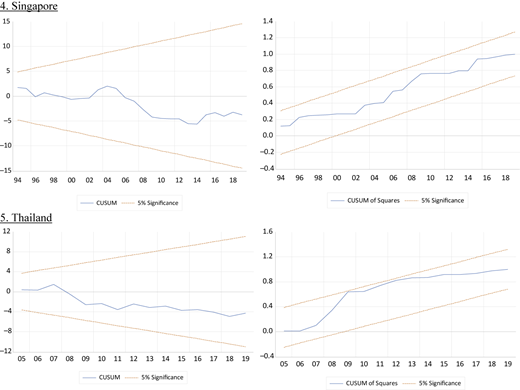
CUSUM and CUSUMSQ graphs. Source(s): The authors
The image shows ten line graphs arranged in five rows and two columns. Each pair of line graphs is labeled for a specific country. For each country, the left graph shows the line for “CUSUM” and the right graph shows the line for “CUSUM of squares,” along with 5 percent significance. The legend is shown at the bottom of each graph. The details of the graphs are as follows: The graphs in the first row are for “Indonesia.” The horizontal axis for both graphs ranges from 2014 to 2019 in increments of 1 year. The vertical axis of the left graph ranges from negative 8 to 8 in increments of 2. The “CUSUM” line starts at (2014, negative 0.63), rises to (2016, 1.5), remains level, and ends at (2019, 1.62). The line for the upper 5 percent significance starts at (2014, 2.5), increases with a positive slope, and ends at (2019, 7.17). The line for the lower 5 percent significance starts at (2014, negative 2.28), decreases with a negative slope, and ends at (2019, negative 6.62). The vertical axis for the right graph ranges from negative 0.4 to 1.6 in increments of 0.4. The line for “CUSUM of Squares” starts at (2014, 0.20), increases to (2016, 0.90), and rises slightly to end at (2019, 1.016). The line for the upper 5 percent significance starts at (2014, 0.56), increases with a positive slope, and ends at (2019, 1.40). The line for the lower 5 percent significance starts at (2014, negative 0.19), increases with a positive slope, and ends at (2019, 0.65). The graphs in the second row are for “Malaysia.” The horizontal axis for both graphs ranges from 1998 to 2018 in increments of 2 year. The vertical axis of the left graph ranges from negative 15 to 15 in increments of 5. The “CUSUM” line starts at (1997, negative 1.16), fluctuates mostly in negative values, reaches a low at (2005, negative 3.22), rises to (2009, negative 0.98), and ends at (2019, 0.047). The line for the upper 5 percent significance starts at (1997, 4.72), increases with a positive slope, and ends at (2019, 13.78). The line for the lower 5 percent significance starts at (1997, negative 4.15), decreases with a negative slope, and ends at (2019, negative 13.22). The vertical axis for the right graph ranges from negative 0.2 to 1.4 in increments of 0.2. The line for “CUSUM of Squares” starts at (1998, 0.097), increases in steps to (2014, 0.77), and ends at (2018, 1.00). The line for the upper 5 percent significance starts at (1998, 0.38), increases with a positive slope, and ends at (2018, 1.32). The line for the lower 5 percent significance starts at (1997, negative 0.22), increases with a positive slope, and ends at (2019, 0.73). The graphs in the third row are for “Philippines.” The horizontal axis for both graphs ranges from 2012 to 2019 in increments of 1 year. The vertical axis of the left graph ranges from negative 10 to 10 in increments of 2. The “CUSUM” line starts at (2012, negative 1.17), rises to (2015, 1.81), fluctuates, and ends at (2019, 2.81). The line for the upper 5 percent significance starts at (2012, 2.82), increases with a positive slope, and ends at (2019, 8.15). The line for the lower 5 percent significance starts at (2012, negative 2.31), decreases with a negative slope, and ends at (2019, negative 7.71). The vertical axis for the right graph ranges from negative 0.4 to 1.6 in increments of 0.4. The line for “CUSUM of Squares” starts at (2012, 0.24), increases in steps to (2016, 0.70), and ends at (2019, 1.02). The line for the upper 5 percent significance starts at (2012, 0.52), increases with a positive slope, and ends at (2019, 1.39). The line for the lower 5 percent significance starts at (2012, negative 0.23), increases with a positive slope, and ends at (2019, 0.66). The graphs in the fourth row are for “Singapore.” The horizontal axis for both graphs ranges from 1994 to 2018 in increments of 2 years. The vertical axis of the left graph ranges from negative 15 to 15 in increments of 5. The “CUSUM” line starts at (1994, 2.25), drops to (2009, negative 3.77), rises slightly, and ends at (2019, negative 3.36). The upper 5 percent significance line starts at (1994, 5.51), increases with a positive slope and ends at (2019, 14.90). The lower 5 percent significance line starts at (1994, negative 4.28), decreases with a negative slope and ends at (2019, negative 13.98). The vertical axis for the right graph ranges from negative 0.2 to 1.4 in increments of 0.2. The line for “CUSUM of Squares” starts at (1994, 0.14), increases in steps to (2009, 0.76), and ends at (2018, 1.01). The upper 5 percent significance line starts at (1994, 0.33), increases with a positive slope, and ends at (2018, 1.30). The lower 5 percent significance line starts at (1994, negative 0.20), increases with a positive slope and ends at (2018, 0.74). The graphs in the fifth row are for “Thailand.” The horizontal axis for both graphs ranges from 2005 to 2019 in increments of 1 year. The vertical axis of the left graph ranges from negative 12 to 12 in increments of 4. The “CUSUM” line starts at (2005, 0.33), peaks at (2007, 1.70), drops to (2011, negative 3.33), and ends at (2019, negative 4.06). The upper 5 percent significance line starts at (2005, 3.60), increases with a positive slope and ends at (2019, 11.09). The lower 5 percent significance line starts at (2005, negative 3.51), decreases with a negative slope and ends at (2019, negative 10.55). The vertical axis for the right graph ranges from negative 0.4 to 1.6 in increments of 0.4. The line for “CUSUM of Squares” starts at (2005, 0.073), increases to (2009, 0.65), and ends at (2019, 0.99). The upper 5 percent significance line starts at (2005, 0.42), increases with a positive slope, and ends at (2019, 1.34). The lower 5 percent significance line starts at (2005, negative 0.22), increases with a positive slope and ends at (2019, 0.68). Note: All numerical values are approximated.CUSUM and CUSUMSQ graphs. Source(s): The authors
4.3 Inferences of the GIRF method: effects of positive and negative FDI shocks on GDP
In this part, we proceed with the responses of the sample countries’ to the positive and negative shocks using GIRF, as shown before (Figure 3). The impulse response will be statistically significant, at the 5% level, once both the mean and confidence interval values are falling above or below zero. We first start by exploring the responses of the sample countries’ to a positive shock. For Indonesia, the positive shock is significant and rises over the 10 periods, and the same thing applies for Philippines. Whereas for Malaysia, the significant positive shock causes to rise for the first four periods, but then falls. In the case of Philippines, the positive shock is significant in the first two periods where falls, and significant from the fifth period again seeing that it vanishes. For the Thailand case, the positive shock is significant starting from the fourth period and causes to rise. On the other hand, for S. Korea and Japan the positive shock is not significant for the entire 10 periods.
 The figure contains 14 line graphs arranged in four rows and two columns. Each pair of graphs is labeled for a specific country, with the left graph titled “Positive F D I shock” and the right graph titled “Negative F D I shock.” The horizontal axis for all graphs is labeled from 1 to 10 in increments of 1. The details of the graphs are as follows: The graphs in the first row are for “Indonesia.” The vertical axis for both graphs ranges from negative 0.005 to 0.020 in increments of 0.005. The graph for “Positive F D I shock” on the left starts at (1, 0.001), rises to (6, 0.006), increases, and ends at (10, 0.010). The graph for “Negative F D I shock” on the right starts at (1, 0.008), peaks at (2, 0.009), then declines to end at (10, 0.001). Both graphs include upper and lower dashed lines for significance bounds. The graphs in the second row are for “Malaysia.” The vertical axis for both graphs ranges from negative 0.005 to 0.010 in increments of 0.005. The graph for “Positive F D I shock” on the left starts at (1, 0.004), increases to (4, 0.008), then gradually declines to end at (10, 0.007). The graph for “Negative F D I shock” on the right starts at (1, 0.008), peaks at (2, 0.008), and gradually decreases to end at (10, 0.001). Both graphs include upper and lower dashed lines representing significance bounds. The graphs in the third row are for “Philippines.” The vertical axis for both graphs ranges from negative 0.000 to 0.010 in increments of 0.005. The graph for “Positive F D I shock” on the left starts at (1, 0.001), increases to (4, 0.004), and gradually rises to end at (10, 0.006). The graph for “Negative F D I shock” on the right starts at (1, 0.001), less gradually, and ends at (10, 0.004). Both graphs include upper and lower dashed lines representing significance bounds. The graphs in the fourth row are for “Singapore.” The vertical axis for both graphs ranges from negative 0.008 to 0.008 in increments of 0.004. The graph for “Positive F D I shock” on the left starts at (1, 0.006), decreases to (3, negative 0.0005), remains nearly flat, and ends at (10, 0.001). The graph for “Negative F D I shock” on the right starts at (1, 0.003), declines to (3, negative 0.007), and ends at (10, negative 0.0035). Both graphs include upper and lower dashed lines representing significance bounds. The graphs in the fifth row are for “Thailand.” The vertical axis for both graphs ranges from negative 0.01 to 0.010 in increments of 0.005. The graph for “Positive F D I shock” on the left starts at (1, negative 0.004), increases to (6, 0.002), remains nearly level, and ends at (10, 0.001). The graph for “Negative F D I shock” on the right starts at (1, 0.001), slightly falls, and stays nearly flat and ends at (10, 0.001). Both graphs include upper and lower dashed lines representing significance bounds. The graphs in the sixth row are for “S. Korea.” The vertical axis for both graphs ranges from negative 0.01 to 0.01 in increments of 0.01. The graph for “Positive F D I shock” on the left starts at (1, negative 0.003), decreases slightly and ends at (10, negative 0.005). The graph for “Negative F D I shock” on the right starts at (1, 0.003), rises to (3, 0.005), and continues to end at (10, 0.006). Both graphs include upper and lower dashed lines representing significance bounds. The graphs in the seventh row are for “Japan.” The vertical axis for both graphs ranges from negative 0.005 to 0.005 in increments of 0.005. The graph for “Positive F D I shock” on the left starts at (1, negative 0.002), decreases to (3, negative 0.004), rises to (7, 0.001), and ends at (10, negative 0.001). The graph for “Negative F D I shock” on the right starts at (1, negative 0.002), increases to (4, 0.00), falls to (6, 0.004), rises, and ends at (10, negative 0.002). Both graphs include upper and lower dashed lines representing significance bounds. Note: All numerical values are approximated.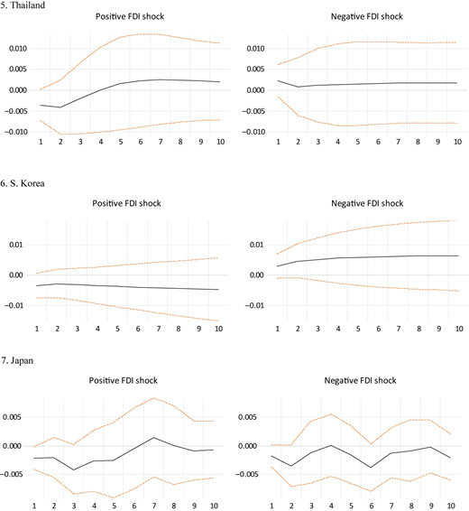
Responses of GDP to positive and negative FDI shocks using GIRF. Source(s): The authors
The figure contains 14 line graphs arranged in four rows and two columns. Each pair of graphs is labeled for a specific country, with the left graph titled “Positive F D I shock” and the right graph titled “Negative F D I shock.” The horizontal axis for all graphs is labeled from 1 to 10 in increments of 1. The details of the graphs are as follows: The graphs in the first row are for “Indonesia.” The vertical axis for both graphs ranges from negative 0.005 to 0.020 in increments of 0.005. The graph for “Positive F D I shock” on the left starts at (1, 0.001), rises to (6, 0.006), increases, and ends at (10, 0.010). The graph for “Negative F D I shock” on the right starts at (1, 0.008), peaks at (2, 0.009), then declines to end at (10, 0.001). Both graphs include upper and lower dashed lines for significance bounds. The graphs in the second row are for “Malaysia.” The vertical axis for both graphs ranges from negative 0.005 to 0.010 in increments of 0.005. The graph for “Positive F D I shock” on the left starts at (1, 0.004), increases to (4, 0.008), then gradually declines to end at (10, 0.007). The graph for “Negative F D I shock” on the right starts at (1, 0.008), peaks at (2, 0.008), and gradually decreases to end at (10, 0.001). Both graphs include upper and lower dashed lines representing significance bounds. The graphs in the third row are for “Philippines.” The vertical axis for both graphs ranges from negative 0.000 to 0.010 in increments of 0.005. The graph for “Positive F D I shock” on the left starts at (1, 0.001), increases to (4, 0.004), and gradually rises to end at (10, 0.006). The graph for “Negative F D I shock” on the right starts at (1, 0.001), less gradually, and ends at (10, 0.004). Both graphs include upper and lower dashed lines representing significance bounds. The graphs in the fourth row are for “Singapore.” The vertical axis for both graphs ranges from negative 0.008 to 0.008 in increments of 0.004. The graph for “Positive F D I shock” on the left starts at (1, 0.006), decreases to (3, negative 0.0005), remains nearly flat, and ends at (10, 0.001). The graph for “Negative F D I shock” on the right starts at (1, 0.003), declines to (3, negative 0.007), and ends at (10, negative 0.0035). Both graphs include upper and lower dashed lines representing significance bounds. The graphs in the fifth row are for “Thailand.” The vertical axis for both graphs ranges from negative 0.01 to 0.010 in increments of 0.005. The graph for “Positive F D I shock” on the left starts at (1, negative 0.004), increases to (6, 0.002), remains nearly level, and ends at (10, 0.001). The graph for “Negative F D I shock” on the right starts at (1, 0.001), slightly falls, and stays nearly flat and ends at (10, 0.001). Both graphs include upper and lower dashed lines representing significance bounds. The graphs in the sixth row are for “S. Korea.” The vertical axis for both graphs ranges from negative 0.01 to 0.01 in increments of 0.01. The graph for “Positive F D I shock” on the left starts at (1, negative 0.003), decreases slightly and ends at (10, negative 0.005). The graph for “Negative F D I shock” on the right starts at (1, 0.003), rises to (3, 0.005), and continues to end at (10, 0.006). Both graphs include upper and lower dashed lines representing significance bounds. The graphs in the seventh row are for “Japan.” The vertical axis for both graphs ranges from negative 0.005 to 0.005 in increments of 0.005. The graph for “Positive F D I shock” on the left starts at (1, negative 0.002), decreases to (3, negative 0.004), rises to (7, 0.001), and ends at (10, negative 0.001). The graph for “Negative F D I shock” on the right starts at (1, negative 0.002), increases to (4, 0.00), falls to (6, 0.004), rises, and ends at (10, negative 0.002). Both graphs include upper and lower dashed lines representing significance bounds. Note: All numerical values are approximated.Responses of GDP to positive and negative FDI shocks using GIRF. Source(s): The authors
Next, we proceed to the effects of the negative shock on the sample countries’ .
The negative shock is not significant for Singapore and Japan. However, for Indonesia and Malaysia, the negative shock is significant and causes to fall over the entire 10 periods. For Philippines and S. Korea, the negative shock is significant but causes to rise. Finally, in the case of Thailand, the GIRF shows that the negative shock is significant but causes the to drop in first two periods and then stays almost steady after that.
Overall, the generalized impulse response function (GIRF) shows that the responses of the sample countries’ to the positive and negative shocks do not seem to be mirror images of one another. This can be interpreted as a sign of the asymmetric impact of on . This conclusion can be supported further by the plots of the Accumulated Response to Generalized one standard deviation Innovations in Figure 3. The plots do show that positive and negative shocks provide different effect on .
5. Concluding remarks
This paper enhances the existing body of literature by investigating whether asymmetrically affects among seven selected Asian countries: Indonesia, Malaysia, Philippines, Singapore, Thailand, South Korea, and Japan. We employed the NARDL model in conjunction with GIRF analysis. From a methodological standpoint, the NARDL model enables the examination of potential asymmetry in how GDP responds to positive and negative shocks, revealing insightful findings that may remain hidden when using a symmetric (linear) analysis. Concurrently, the GIRF analysis allowed us to evaluate the dynamic responses of to both positive and negative shocks.
The NARDL model findings indicated that in the long term, shocks asymmetrically affect the of five Asian countries: Indonesia, Malaysia, Philippines, Singapore, and Thailand. Conversely, the presence of short-run asymmetry was only confirmed for Malaysia, Thailand, and Japan. The GIRF estimations, on a general note, demonstrated that a positive shock appears to significantly influence the of most sample countries, while a negative shock has a relatively minor impact. Therefore, the GIRF analysis provides further additional evidence supporting the asymmetric influence of shocks on across the selected Asian countries. In conclusion, when examining the repercussions of fluctuations on a country’s , it is essential to account for asymmetry in the analysis; otherwise, the empirical procedures may lack proper specification and raise doubts concerning the reliability of the findings. Overall, the results reveal nonlinear and context-specific responses in both advanced and emerging markets, indicating that FDI impacts are neither uniform nor linear. This underscores the importance of designing economic policies that consider each country’s structural characteristics and institutional context. Our analysis further demonstrates that FDI shocks can produce heterogeneous outcomes, depending on the direction of inflows and the country’s absorptive capacity.
Several policy implications would emerge based on our empirical results. First, we propose that to maximize the benefits of positive FDI shocks, host countries should strengthen absorptive capacities through targeted investments in human capital development, innovation ecosystems, and financial sector reforms. Specifically, we now recommend that governments prioritize policies such as improving the quality of education and workforce skills, investing in innovation and research infrastructure, creating a more stable and attractive environment for long-term foreign investment, strengthening financial market development to facilitate investment absorption, and enhancing institutional transparency and governance to retain high-value foreign investors. Second, to mitigate the adverse effects of negative FDI shocks, we suggest diversifying FDI sources, promoting domestic investment as a buffer, supporting domestic entrepreneurship and SMEs to reduce dependency on foreign capital, and establishing contingency policies such as countercyclical fiscal measures to sustain growth momentum during downturns and to cushion against external FDI volatility. Third, our findings are relevant to governments that embrace open economic policies, underscoring the need for them to allocate added consideration to the FDI-sector-based analysis (i.e. education, health, industry, infrastructure, and telecommunication). Fourth, the findings from our control regressors indicate the importance of the government’s monetary, fiscal, and societal standings committed to such robust key factors. These factors encompass the development of national human capital, adjustments to trade-openness policies, and careful consideration of the country’s demographic shifts—such as population growth rate, population age structure, and per capita income levels.
For future research, although FDI appears to have an asymmetric impact on the real GDP on the aggregate level of data across Asian countries, however, this dynamic may differ when conducting a sectoral-specific analysis among these countries. Forthcoming research could adopt an analysis approach utilizing detailed sectoral-level data or may incorporate FDI stock data to further enrich the understanding of FDI’s asymmetric effects on sustainable GDP growth across Asian countries. Similarly, future research could highlight whether the empirical long- and short-run FDI asymmetric results vary by utilizing diverse types of population growth. Furthermore, future research could incorporate a wider array of control variables such as a country’s income level, population size, and population age structure which could certainly contribute to more robust assessments of the FDI-growth relationship.
Notes
Likewise, on a country-specific basis, see, Fadhil and Almsafir (2015) for Malaysia; Peng et al. (2016) for China; Luu et al. (2017) for Vietnam; Sothan (2017) for Cambodia; Sunde (2017) for South Africa; Choi and Baek (2017) for India; Reza et al. (2018) for Bangladesh.
The preconditions may include the country’s level of income (Alvarado et al., 2017), having well-developed financial markets (Osei and Kim, 2020); input accumulation (Makiela and Ouattara, 2018); human capital (Fadhil and Almsafir, 2015); appropriate political conditions (Magazzino and Mele, 2022); economic growth (Odhiambo, 2021; Maryam and Mittal, 2020; Gherghina et al., 2019; Mittal and Mittal, 2019; Asongu et al., 2018).
The main reason for the sample selection is that Indonesia, Malaysia, Philippines, Singapore, and Thailand were among the founding members of ASEAN, established in 1967, beside the data is mainly available for these countries.
For recent applications of the NARDL model, kindly see: Kisswani and Kisswani (2019), Kisswani (2021a, b), Kisswani and Elian (2021), Kisswani (2024), Kisswani and Khan (2023), Kisswani et al. (2022).
For the F-statistics test, Pesaran et al. (2001) provided upper bound and lower bound critical values. The F-statistics needs to be higher than the upper bound critical value for cointegration evidence. For more details, kindly see: Kisswani (2019), Kisswani et al. (2019, 2020).
For more details, see Bai and Perron (1998).
Although Table 6 reports the long-run coefficients for all variables, our focus is on the long-run coefficients of and .
The supplementary material for this article can be found online.

