

We propose a method for calibrating high-dimensional parameters in the Hull–White one-factor model using market prices of swaptions, aimed at generating mark-to-market interest rate scenarios in the Korean insurance industry. Our approach integrates a trust region-based Bayesian optimization technique with a parameter space decomposition method to solve the calibration problem. Empirical studies demonstrate that our method achieves superior stability and effectiveness in calibrating high-dimensional parameters compared to conventional Bayesian optimization approaches.
1. Introduction
Recently, the South Korean insurance industry has undergone substantial regulatory transformations with the adoption of the new International Financial Reporting Standard 17 (IFRS17). Regulators decided to adopt the Korean Insurance Capital Standard (K-ICS), a new financial soundness indicator, to cope with such changes. Given these changes, there has been a pressing need for advanced interest rate scenario models that accurately reflect the unique features of K-ICS. This study proposes a calibration method that effectively calibrates high-dimensional [1] parameters in interest rate models, ensuring a more precise assessment of capital solvency under the new regulatory framework.
The transition from International Financial Reporting Standard 4 (IFRS4) to IFRS17, effective January 2023, has significantly transformed insurance accounting practices. Under IFRS4, insurance liabilities were evaluated based on historical costs, which often led to financial discrepancies when interest rates showed big fluctuations. IFRS17 resolves this issue by requiring liabilities to be assessed at current market rates, which necessitates regular updates to discount rates and relevant assumptions. This change enhances transparency and ensures that financial statements reflect economic conditions more accurately. Additionally, IFRS17 modified the timing of revenue recognition to align with the coverage period of insurance contracts, thereby smoothing income statements and providing a clearer view of an insurer’s financial stability.
Correspondingly, a new solvency system has been introduced to incorporate the change in accounting standards. In South Korea, K-ICS has replaced the Risk-Based Capital (RBC) framework, aiming for regulatory enhancement. Unlike RBC, which primarily measured financial health by comparing available capital to required capital, K-ICS adopts a market value-based assessment of insurance liabilities. This approach aligns with the international standards developed by the International Association of Insurance Supervisors. The new solvency system offers a more realistic and dynamic assessment of an insurer’s financial stability, especially in response to market fluctuations.
Accordingly, it is essential to consider an interest rate scenario model that is suitable for the evolving domestic insurance supervision environment, driven by the introduction of IFRS17 and K-ICS. Recent research has begun to address interest rate risk measurement under the new regulatory framework. Noh et al. (2019) compared the dynamic Nelson-Siegel (DNS) and arbitrage-free Nelson-Siegel (AFNS) models, demonstrating that the AFNS can result in lower capital requirements through improved asset-liability matching. Lee and Ki (2019) reviewed the arbitrage-free DNS shock-generating algorithm used in K-ICS 2.0, highlighting potential improvements in managing interest rate shocks more effectively. Ryu and Yu (2020) analyzed the financial impacts of hybrid bond issuances by insurance firms, revealing nuanced effects on solvency and performance. Jeong (2022) proposed copula-based internal models for risk aggregation under K-ICS, offering a method to evaluate required capital through more accurate risk correlation assessments. Noh (2024) discussed the adoption of internal models under K-ICS, emphasizing their suitability for reflecting individual company risks and fostering a risk-focused management culture. Despite these advances, the field remains in its early stages, offering substantial opportunities for further exploration and development. A well-constructed model can facilitate research on shock scenario calculations for interest rate curves, crucial for financial risk assessment.
In the context of K-ICS, the calibration of interest rate models serves a distinct purpose compared to the conventional focus on hedging exotic interest rate derivatives. Unlike financial firms that actively engage in dynamic hedging of optionality within their liabilities, life insurance companies operate under a different paradigm. Their primary objective is to value insurance contracts accurately for risk measurement purposes rather than to match the model to the optionality embedded in their liabilities. As a result, reflecting overall market conditions precisely takes precedence over replicating specific optionality patterns [2].
Among the diverse interest rate models that could be employed depending on various circumstances (Brigo and Mercurio, 2006), this study focuses on the Hull and White (1993) one-factor model, widely employed by South Korean insurance companies for its adaptability and effectiveness in reflecting current market conditions and meeting regulatory requirements. Before the adoption of K-ICS, non-stochastic interest rate models were often utilized for scenario generation. However, with the introduction of K-ICS, which requires full fair value evaluation of assets and liabilities (Noh et al., 2024) [3], stochastic interest rate models became essential to accurately reflect market conditions. Among these, the Hull–White one-factor model stands out as a parsimonious yet robust choice for meeting regulatory standards. According to the KIDI, currently about 30 insurance companies and Saemaul Geumgo are utilizing the Hull–White one-factor model along with ESG Pro to generate scenarios [4]. Organizations like Shinhyup and Suhyup are also planning to adopt this approach. By increasing the number of parameters in the Hull–White one-factor model, more accurate calibration becomes feasible, which naturally leads to more precise results in scenario generation. This enhanced accuracy is essential for fulfilling the requirements of K-ICS, as it ensures that the generated scenarios more closely reflect actual market conditions.
As the Hull–White one-factor model inherently includes time-varying parameters, those continuous-valued parameters are often approximated using step functions with respect to the time variable for practical purposes. Such step functions may require defining more than 10 constant parameters. The calibration methodology proposed in this paper proves robust for calibrating such interest rate models with high-dimensional market parameters.
The calibration of the Hull–White interest rate model has been extensively studied, and various methodologies have been proposed over the years. Traditional approaches often involve calibrating the model parameters using optimization algorithms like the Levenberg–Marquardt method, as presented in Hull and White (2001), which is commonly used in practice in South Korea according to Korea Insurance Development Institute (KIDI) guidelines (KIDI, 2013) [5]. However, these methods face limitations when dealing with time-dependent parameters due to increased computational complexity and the high dimensionality of the calibration problem.
Recent studies have explored advanced optimization techniques and machine-learning approaches to address these challenges. Hernandez (2016) has proposed a calibration framework that utilizes a neural network to approximate the objective function, transforming the calibration problem into an optimization problem searching for a minimizer of the inverse approximate function. This approach was validated through experiments employing the Hull–White one-factor model. Ruf and Wang (2019) have reviewed further relevant papers which employed neural networks to approximate pricing functions and accelerate the calibration process. Kladívko and Rusỳ (2023) have suggested a calibration method for Hull–White one-factor model based on the maximum likelihood estimation by fitting time-dependent model parameters to a market forward rate curve. Russo and Torri (2019) have developed a calibration technique for the Hull–White one-factor and two-factor models, based on pricing formulas for coupon bond options and swaptions, under the assumption of a deterministic (i.e. constant over time) mean reversion rate and volatility. Others have utilized automatic differentiation and adjoint methods to efficiently compute gradients in high-dimensional settings (Schlenkrich, 2012; Griewank and Walther, 2008).
While these methods offer improvements, they often rely on strong assumptions (e.g. fixing certain parameters or simplifying the model structure) or are tailored to specific situations. Our methodology advances the existing literature by assuming both the mean reversion rate and volatility as piecewise constant and by effectively tackling the high-dimensional calibration problem under these conditions without imposing restrictive assumptions, making it more broadly applicable.
Bootstrapping is a widely adopted method for calibrating the Hull–White one-factor model in practice, as it simplifies the high-dimensional problem into a sequence of lower-dimensional tasks. By sequentially fitting the model parameters (i.e. the mean reversion rate and volatility) to subsets of the swaption price table—–such as specific rows, columns or diagonals—–bootstrapping circumvents the need to solve the full optimization problem at once. However, this approach has notable limitations. First, it does not fully utilize the entire market data available, as only subsets of the swaption price table are employed at each step of solving subproblems. This partial utilization may result in a failure to capture overall market dynamics.
Another challenge with bootstrapping is the risk of parameter inconsistencies due to its sequential nature. Since calibration is performed step by step, some swaption prices are reused multiple times across different estimation steps. Specifically, in the early stages, parameters are estimated using only shorter-maturity swaption prices, and these values are then carried forward and reused in subsequent steps when estimating parameters for longer maturities. However, because each estimation step optimizes parameters independently rather than in a globally consistent manner, the same parameters (i.e. the mean reversion rate and volatility) may be assigned slightly different values depending on the subset of data used in each step. This sequential dependency can introduce minor inconsistencies in the final calibrated values, leading to potential instability in the overall calibration process.
A proper establishment of an interest rate model requires both the mathematical derivation for product price calculations and the calibration of model parameters. Because the relationship between parameters and prices is typically not explicitly identified, this calibration procedure often becomes a black-box optimization problem. Function approximation methods are commonly employed to solve such problems, serving as alternatives to gradient-based or heuristic algorithms (Snoek et al., 2012). Bayesian optimization (BO), in particular, offers a robust solution when evaluations of the objective function are costly and noisy, conditions that are frequently encountered in financial modeling.
Nevertheless, interest rate models with high-dimensional market parameters pose challenges for the application of general BO. Recently, significant research has been conducted on high-dimensional BO—often referred to as such when involving dimensions over 20—to address similar issues in various domains (Malu et al., 2021; Binois and Wycoff, 2022). The relevant studies could be categorized into two main research streams; one focusing on Gaussian Process (GP) modeling, and the other on acquisition function optimization. In the realm of GP modeling, Chen et al. (2012) developed a framework for joint optimization and variable selection in high-dimensional settings and showed that it could provide strong performance guarantees. Additionally, Duvenaud et al. (2011) introduced the concept of additive GPs, which decompose functions into sums of low-dimensional functions for enhanced interpretability and predictability. Regarding acquisition function optimization, Eriksson et al. (2019) proposed a trust region-based BO algorithm, employing local BO for scalable global optimization, effectively managing large-scale high-dimensional problems. Similarly, Gupta et al. (2020) proposed a method that maximizes the acquisition function over a discrete set of low-dimensional subspaces to maintain accuracy and efficiency in larger search spaces.
Aligning with these advancements, we propose a parameter calibration method specifically tailored for the high-dimensional model parameter calibration problem in insurance company interest rate models. Our approach combines two distinctive strategies from the aforementioned research streams; pairwise decomposition of the input space, inspired by GP modeling techniques, and trust region-based sample search, relevant to the acquisition function optimization. The proposed method efficiently reduces the complexity of the model space by distinguishing the effects of variables across specific periods or timestamps. Additionally, our approach dynamically adjusts the search space, significantly enhancing the accuracy and efficiency of the optimization process for the acquisition function. This synergistic integration enables more effective and efficient exploration of the parameter space, leveraging the strengths of each method to enhance the robustness and accuracy of the model. Our numerical experiments demonstrated that our approach can calibrate the parameters of the interest rate model more accurately, developed to meet the stringent standards, IFRS17 and K-ICS, compared to the conventional BO.
Here, we summarize the contributions of this study.
- (1)
We propose a high-dimensional model parameter calibration method for the Hull–White one-factor model which is commonly employed by South Korean insurance companies. Our method integrates the trust region-based BO with the pairwise decomposition of the parameter space. This enhances the efficiency and accuracy of parameter calibration in high-dimensional settings, addressing the challenges posed by the complex structure of interest rate models under the new regulatory framework.
- (2)
Through numerical experiments, we demonstrate the effectiveness of the proposed method in calibrating high-dimensional parameters of the interest rate model. By fitting the model to market prices obtained using Bloomberg swaption data, our approach not only achieves better calibration accuracy compared to the conventional BO but also exhibits robustness and stability across different market conditions.
The remainder of the paper is organized as follows. Section 2 describes the swaption and investigates the specific value of interest that we aim to calibrate via the interest rate model. Section 3 derives the swaption pricing formula under the Hull–White one-factor model and proposes the calibration method for high-dimensional model parameters. Section 4 presents experimental results using Bloomberg swaption data and conducts relevant discussions. Finally, Section 5 provides a conclusion and suggests future research topics.
2. Problem description
In this study, we develop an interest rate model for scenario generation focusing on swaptions and investigate the method for calibrating the model parameters. A swaption provides the holder with the right to enter into a swap contract with a specific maturity at a predetermined time. We refer to a swaption with an option maturity of Tn and an underlying swap maturity of TS as a Tn × TS swaption. A payer swaption gives the holder the right to initiate a payer swap contract. Therefore, a payer swaption can be viewed as a call option with the swap rate as the underlying asset.
The payoff structure of a payer swaption with a strike price K for a Tn × TS swaption is as follows:
Here, [x]+ denotes the maximum value between 0 and x (i.e. [x]+ = max{0, x}), and TN = Tn + TS. D(t, T) is the price of a zero-coupon bond maturing at T as seen from time t, and ΔY is the day count fraction (or period) for the swap payments. We define total payment counts as n = Tn/ΔY and N = TN/ΔY. Pn+1,N(Tn) is the present value of a basis point and is calculated as . This can be interpreted as the increase in the value of the swap from the perspective of the fixed-rate receiver when the fixed-rate increases by one unit. The forward par swap rate is denoted as yn,N(Tn) = (D(Tn, Tn) − D(Tn, TN))/Pn+1,N(Tn), which represents the fixed-rate that makes the value of an interest rate swap starting at Tn with a maturity of TS zero at the current time.
Therefore, the value at time t of a payer swaption with a strike price K can be expressed as the conditional expectation under the risk-neutral measure Q, denoted as , as follows:
Expressing this in terms of the expectation under the swap measure Qn+1,N, which takes Pn+1,N(t) as the numeraire, it can be rewritten as follows:
Similarly, the value of a Tn × TS receiver swaption at time t can be expressed as follows:
A swaption with a strike price equal to the forward par swap rate is called an at-the-money-forward swaption, where the strike price is K = yn,N(0). In this case, the values of the payer swaption and the receiver swaption are equal. That is, the following equation holds:
In this study, we use these at-the-money-forward swaptions and henceforth denote the value of a Tn × TS payer swaption as PS(Tn, TS). Therefore, we explore the calibration process by selecting an appropriate interest rate model to fit the actual prices of these instruments. While the calibrated model can be used for generating future interest rate scenarios, such an application is beyond the scope of this study and will not be discussed directly within this paper.
3. Methodology
As described in Section 1, this study utilizes the Hull–White one-factor model for interest rate modeling and parameter calibration. Since this model includes parameters that vary over time, the number of parameters to be calibrated increases when analyzing longer periods. In this section, we propose a calibration method for fitting this model to swaption prices. Section 3.1 derives the swaption price assessment formula under the Hull–White one-factor model. Section 3.2 formulates the parameter calibration problem to match the prices from the assessment formula and market. Section 3.3 illustrates the BO-based solution method for the high-dimensional calibration problem.
3.1 Hull–White one-factor model
We begin with deriving the swaption pricing formula under the Hull–White one-factor model. The derivation largely follows Schrager and Pelsser (2006). The Hull–White one-factor model allows the mean reversion rate α and the volatility σr to vary over time. The instantaneous short rate is described by the following stochastic differential equation (Hull and White, 1990):
Here, the function θ(t), which is calibrated to fit the initial term structure of interest rates, is given by Andersen and Piterbarg (2010):
where f(t, T) is the forward rate for the interval (t, T). By defining a(t) ≔ r(t) − f(0, t), the dynamics of a(t) and the bond reconstitution formula are given as follows (Andersen and Piterbarg, 2010):
With the payer swaption price in Equation (1), the dynamics of yn,N(t) under the swap measure Qn+1,N can be expressed using Ito’s lemma as follows:
where
Following Schrager and Pelsser (2006), we use the following approximations:
and this leads to the approximate value of ∂yn,N(t)/∂x, which we denote as , as follows:
Accordingly, the swap volatility becomes deterministic with respect to time, and consequently, the swap rate is a Gaussian martingale. Under the above assumption, yn,N(t) at t = 0 follows the following probability distribution:
As a result, the at-the-money-forward payer swaption price with K = yn,N(0) is calculated as follows:
Note that this price calculation relies on the model parameters α(t) and σr(t).
3.2 Formulation of the parameter calibration problem for swaption price matching
Here, we formulate the optimization problem for calibrating the Hull–White one-factor model parameters using the swaption price formula in Equation (4). To do so, we first determine the cash price of the swaption from the market-quoted volatility.
Financial data vendors, such as Bloomberg, generally provide two types of volatilities; normal volatility and Black volatility. In this study, we use the Black volatility to derive the market transaction price because it is more widely used by domestic insurance companies, and interest rates are generally assumed to be positive except on rare occasions.
The market price of a payer swaption can be derived using the swaption pricing formula from the Black model by substituting the Black volatility σB. The market transaction price of a Tn × TS payer swaption, PSM(Tn, TS), is calculated as follows:
with
where is the cumulative distribution function of the standard normal distribution.
Now, we can calibrate the parameters of the Hull–White one-factor model so that the corresponding swaption price matches that of the Black model. For a certain date (or a moment), we define the set of maturity pairs of interest as follows:
where the index i specifies the maturity pair. Here, is the number of maturity pair combinations. We denote the market price of the swaption corresponding to the i-th maturity pair as follows:
For all these pairs, we aim to minimize the average squared errors between the market price and the price determined from the Hull–White one-factor model. Thus, the calibration problem for price matching can be formulated as follows:
Note that the market price is considered given because it can be calculated from the Black model as in Equation (5). Solving this minimization problem is equivalent to finding the Hull–White one-factor model parameters such that the resulting price, calculated as illustrated in Section 3.1, closely resembles the market price.
3.3 High-dimensional Bayesian optimization for the parameter calibration
In the optimization problem defined in Equation (6), the parameters α(t) and σr(t) are assumed to be time-varying continuous functions. Given the limited data available, calibrating (or fitting) these continuous functions could either be infeasible or lead to severe overfitting. Thus, we assume these functions to be piecewise constant, and accordingly, approximate the formula used in swaption valuation. Specifically, we assume that α(t) and σr(t) are constants within intervals defined as follows:
where the boundaries of these intervals are defined by with the total number of intervals Nitv.
Under this assumption, the swaption price in Equation (4) could be calculated with σy(Tn) value as follows:
for maturity Tn belonging to the interval [tj, tj+1). In the case of j = 1, the first summation term is omitted. The values of can be calculated using Equation (3), where B(t, Ti) and DP(0, Ti) values are derived from Equation (2) by plugging in the piecewise constant parameters α(t) and σr(t). While the derivation of DP(0, Ti) is straightforward and thus omitted, the calculation of B(t, Ti) is shown below:
where t ∈ [tj, tj+1) and Ti ∈ [tk, tk+1). However, as deriving the final swaption price formula of PSHW under this assumption results in overly complex expressions, we do not explicitly present the full formula here.
With this discretization, the calibration problem in Equation (6) transforms into:
where its decision variables are no longer continuous functions but rather vectors of dimensions 2Nitv (i.e. ). Notably, even in the transformed problem, there is no explicit formula describing the relationship between these decision variables and the objective function or the average squared error. This makes the calibration problem for swaption price matching a black-box optimization problem.
This type of problem is ideally suited for BO, which leverages a GP to model the relationship between decision variables and the objective function probabilistically. BO uses the GP model to calculate an acquisition function, which strategically guides the search for optimal solutions by effectively balancing the exploration of new solution spaces with the exploitation of regions anticipated to yield minimal error. However, BO is inefficient for high-dimensional problems, typically when dimensions exceed 20 (Malu et al., 2021). This is because the solution space exponentially increases with the input dimension, degrading the exploration-exploitation balance (Binois and Wycoff, 2022). To mitigate these risks and enhance the efficiency of our optimization strategy, we integrate two approaches; trust region-based BO, similar to Eriksson et al. (2019), and a pairwise decomposition of the input space.
For the conventional BO, the GP should be modeled with respect to a vector , which includes all model parameters, as an input variable. With the mean and covariance functions μcon and κcon, the GP of the conventional BO, denoted as fcon, is expressed as follows:
Given the observation of inputs (i.e. the model parameters) and outputs (i.e. the average squared errors) [6], represented as dataset , the posterior of the function fcon is also Gaussian. That is, the following holds (Williams and Rasmussen, 1995):
where the posterior mean and covariance of the inputs for evaluation are given by:
with the vector and the matrix Kcon(x1, x2) having its i-th row and j-th column element as κcon(x1,i, x2,j) for 1 ≤ i ≤ |x1| and 1 ≤ j ≤ |x2|. Here, no observation noise is assumed as the average squared error can be precisely calculated. The GP fcon approximates the relationship between the model parameters and the average squared error in Equation (7). Note that later on in the numerical experiments, this conventional BO will serve as a benchmark model.
Alternatively, we develop a different approach for modeling the relationship by representing it as a sum of multiple GPs, each constructed upon mutually exclusive and exhaustive subsets of entire model parameters. Specifically, we model an individual GP such that the j-th GP, denoted as fj, considers the pair of parameters (αj, σr,j) in the j-th time interval [tj, tj+1) as an input variable. The proposed GP, f, can be expressed in an additive form of these individual GPs as follows:
Again, μj and κj denote the mean and covariance functions of the j-th GP, respectively.
For this additive model [7], where each fj is an independently modeled GP, the posterior distribution of f is also Gaussian because GPs are closed under addition. Given the dataset , the posterior distribution is expressed as:
where the posterior mean and covariance functions are calculated as follows:
with
Here, the vector μj(x′) and matrix Kj(⋅,⋅) are calculated as similar to μcon(x′) and matrix Kcon(⋅,⋅), but with respect to j-th mean and covariance functions (i.e. μj and κj). Additionally, it is noticeable that these calculations only account for j-interval’s parameters (i.e. αj and σr,j) even though they are expressed with inputs x′ or x.
This approach ignores the joint effects between different time intervals, such as interactions between the following pairs; (αj, αj′), (σr,j, σr,j′), and (αj, σr,j′) for j ≠ j′. It only focuses on the effect within a single interval. Despite this, the overall behavior of the system is influenced by an implicit aggregation of individual models. As a result, the swaption price from the Hull–White one-factor model is expressed as a probabilistic distribution over the entire input space. This modular approach reduces computational complexity by treating different intervals independently, yet empirically, it still effectively optimizes across the entire solution space.
Next, we describe how we further extend the aforementioned approach for handling the high-dimensional input space more effectively. After GP modeling, sampling solution candidates are necessary for optimizing the acquisition function. Typically, the conventional BO involves sampling from the entire input sample space, which is a 2Nitv-dimensional vector space of an input x in our problem. Borrowing the concept of trust region Bayesian optimization (TuRBO) (Eriksson et al., 2019), we adapt a trust region-based sampling technique upon the decomposition-based GP.
We dynamically adjust the search space, referred to as the trust region, based on the outcome of optimization attempts. This adjustment is performed separately for the corresponding parameter pair of each time interval rather than for the entire input space. Let lj represent the size parameter of the trust region for the j-th input pair, (αj, σr,j), which determines the actual size of the region based on its structural properties (e.g. the radius of a ball-shaped region or the length of a side in a cube-shaped region). Specifically, we adjust lj depending on whether there was a performance improvement in the previous iteration of BO as follows:
where γinc > 1 and γdec < 1 are factors controlling the expansion and contraction of the trust region, and lmax and lmin represent the maximum and minimum allowable sizes. In this strategy, if the previous iteration was successful—indicating potential near the current region—we increase lj to expand the search space, potentially capturing more of the local optimum’s vicinity. Conversely, if the optimization was not successful, lj is decreased to refine the search area, focusing more narrowly on promising regions.
High-Dimensional Bayesian Optimization for Solving the Parameter Calibration Problem
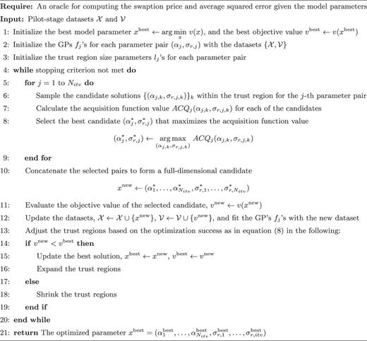
Put together, Algorithm 1 provides a structured approach to our optimization method. The algorithm begins by conducting a pilot sampling of the 2Nitv-dimensional vector across the entire input domain. This initial sampling forms the input parameter set . We then construct the set of objective values for the parameter calibration problem, where each element v(x) represents the average squared error in Equation (6), calculated using the swaption price formula in Equation (4). Using these initial datasets of inputs and outputs, and , individual GPs fj are fitted for each parameter pair (αj, σr,j). The size parameters for the trust regions, lj’s, are also initialized.
Subsequent steps are iteratively repeated until a stopping criterion is met, with each step being performed separately for each parameter pair indexed by j. This separation ensures that the sampling, acquisition function evaluation, and selection of candidates for each pair are conducted independently of the others. For each parameter pair subspace, candidate solutions (αj,k, σr,j,k), with k denoting the candidate index, are sampled within the current trust region using the Latin hypercube sampling. The acquisition function values, denoted by ACQj(⋅), are then calculated for each candidate relative to its respective GP, fj. Among these candidates, the one that maximizes the acquisition function is chosen as the best candidate, denoted as . These optimal pairs are concatenated to form the entire model parameters for the original input space, . Under this configuration, the objective value (i.e. average squared error) is evaluated, and each individual GP is updated accordingly. Depending on whether this new parameter vector achieves a lower error than the best error previously recorded, the trust regions are either expanded or contracted.
4. Numerical experiments
This section presents the experimental results of calibrating interest rate model parameters using swaption products in South Korea via the proposed method. Section 4.1 details the experimental settings, including the data descriptions and assumptions. Section 4.2 provides a comprehensive presentation of the results, highlighting the strengths of the proposed method through comparisons with the benchmark model.
4.1 Experimental settings
This section presents the detailed experimental settings. For clarity, it is divided into two parts: Section 4.1.1 provides a comprehensive description of the data used in this study, including market-quoted volatilities, market transaction prices and interest rate curves. Section 4.1.2 outlines the calibration parameters and other general settings related to the proposed method.
4.1.1 Data description
This study focuses on swaptions with swaps as the underlying assets. Specifically, we used data obtained from Bloomberg, leveraging (implied) Black volatilities from the Bloomberg Interest Rate Composite. These volatilities are quoted with tickers formatted as KWSV BVOL Curncy XXYY, where XX and YY denote the swaption and underlying swap maturities, Tn and TS, respectively. The swaption maturities considered are Tn = 1, 2, 3, 5, 7, 10 years, and the underlying swap maturities are TS = 1, 2, 3, 5, 7, 10 years, resulting in a total of maturity pairs. The market-quoted volatilities, σB, are utilized in the Black model to compute the corresponding market transaction prices (or cash prices), PSM(Tn, TS), as described in Equation (5). These cash prices are then used in the objective function value calculation of the calibration problem in Equation (7). The dataset spans from January 10, 2018, to November 29, 2023, using weekly closing prices on Wednesdays for a total of 308 observation days.
In the Korean capital market, derivatives relying on government bond yields are rare, with the exception of government bond futures. Thus, we use swaptions as a proxy for calibration. However, if products relying on government bond yields that accurately reflect the term structure of volatilities were available, they would naturally be considered as calibration targets.
In general, the insurance capital standard (ICS) and Solvency II utilize interest rate swaps (IRS) to generate interest rate curves. However, in South Korea, a peculiar phenomenon occurs where the IRS, which includes credit risk, often shows lower rates than government bonds due to the interest rate swap inversion phenomenon (Lim and Jang, 2007). Therefore, this study used government bonds to derive the initial discount rate curve, aligning with the recent ICS field test method. The data period, similar to the swaption data, spans from January 10, 2018, to November 29, 2023. The maturities range from 1 year to a maximum of 20 years, which corresponds to the sum of the maximum swaption maturity Tn and the maximum underlying swap maturity TS. Because the available government bond yield data does not cover all maturities, we employed the Smith–Wilson method (Smith and Wilson, 2001) to interpolate the missing maturities. Specifically, the zero rates for 1, 2, 3, 5, 10 and 20 years are directly obtained, while the rates for the remaining maturities are interpolated. The resulting interest rate curve is depicted in Figure 1, where the solid line represents the original zero rates, and the dashed line indicates the interpolated values.

4.1.2 General experimental setup
For the model parameter calibration, the upper bound of the time interval is set to 20 years, which is the sum of the maximum swaption maturity Tn and Ts. We assume that both α and σr are piecewise constant with an interval length of one year. For long-term parameters beyond 10 years, the values are assumed to be constant (i.e. αi = α10 and σi = σ10 for 11 ≤ i ≤ 20). Therefore, the parameters to be calibrated consist of the vector (α1, …, α10, σ1, …, σ10), with 20 elements in total. This setup is designed to ensure the benchmark model operates moderately, as the conventional BO typically begins to struggle with dimensions approaching 20. Nonetheless, we would like to note that the proposed method is capable of handling parameter dimensions larger than 20 (e.g. time domain partitioning on a monthly basis).
As mentioned earlier in Section 3.3, we use the conventional (or plain) BO without any enhancement as a benchmark model. This approach involves using a 20-dimensional parameter vector as the input variable for GP modeling and searching for candidate solutions across the entire input domain. Both the proposed method and the benchmark model utilize 200 randomly sampled parameters as pilot samples for the initial GP modeling. Initially, these samples were drawn with α and σr values from [0,1]. However, we observed that α > 0.03 or σr > 0.04 resulted in poor model performance. Therefore, we have set the domain of the model parameters [8] . The lower bound is set to 10–3 to prevent errors in the swaption price calculation and to ensure the model behaves within a reasonable context. The stopping criterion for the optimization process is defined as reaching a maximum of 50 iterations or the occurrence of no performance improvements for five consecutive iterations. The size parameters for the trust regions were initialized as lj = 0.8 for all j = 1, 2, …, 10, with γinc = 1.1, γdec = 0.9, lmax = 2.0 and lmin = 0.5.
Finally, we use the expected improvement (EI) as the acquisition function. The EI for a point x given a GP posterior with mean μ(x) and variance σ2(x), and the best solution candidate up to far xbest is calculated as:
where is the probability density function of the standard normal random variable. For the benchmark model, x represents a 20-dimensional vector of all parameters. In the proposed method, the EI is calculated for each GP fj with respect to the corresponding parameter pair xj = (αj, σr,j).
4.2 Experimental results
Under the settings described earlier, we performed the parameter calibration using both the proposed method and the benchmark model. Figure 2 shows the objective function value after the optimization. Recall that the objective function is the average squared error in Equation (6) across all (Tn, TS) combinations. Throughout the testing period, the proposed method consistently achieves a better solution, with an average of 46.235% lower error than the benchmark model.

This trend is further corroborated by the statistics of the objective function values over the testing period, as shown in Figure 3. The plot illustrates the yearly average of the objective function values along with their corresponding standard deviations. The proposed method not only consistently demonstrates a lower calibration error compared to the benchmark model but also exhibits reduced variability. Specifically, the smaller standard deviations observed in the proposed method indicate higher stability in calibration results across different time periods. This suggests that the proposed method is not only more accurate but also more reliable, which is critical for practical applications in risk management.

These improvements confirm that employing individual GPs via pairwise decomposition of the input space, as outlined in Section 3.3, aids the optimal parameter search process despite ignoring joint effects between different time intervals. This suggests that while the accuracy of surrogate modeling might decrease compared to using vectors of entire parameters, the advantages in terms of improved exploration–exploitation balance significantly outweigh the drawbacks.
Next, we investigate the time-average performance for each specific maturity pair. For each maturity pair, we compute the squared percentage error between the market price and the model price at each time point over the evaluation period. We then average these errors across all time points. That is, we calculate the time-averaged mean squared percentage error (MSPE) for each swaption maturity pair. The results are presented in Table 1.
Time-averaged performance comparison for each maturity pair
| Tn\TS | 1 | 2 | 3 | 5 | 7 | 10 |
|---|---|---|---|---|---|---|
| 1 | 4.5648/11.9618 | 1.3698/21.8410 | 0.7137/22.4873 | 0.5816/18.0907 | 1.0917/16.9350 | 1.5537/16.2323 |
| 2 | 14.3426/12.4134 | 2.4706/7.1413 | 0.6178/8.8432 | 0.9775/11.8410 | 2.7375/15.1261 | 4.3994/16.8990 |
| 3 | 22.0335/21.9966 | 5.9828/7.7694 | 1.2249/4.2516 | 1.3701/5.7262 | 4.3304/9.4019 | 7.4622/12.4973 |
| 5 | 32.4725/34.4908 | 12.5185/17.1694 | 3.9538/10.4634 | 1.1257/10.0113 | 4.7915/13.8504 | 8.3897/16.2631 |
| 7 | 34.7667/30.7702 | 16.2570/13.8607 | 6.8555/8.1459 | 0.8705/10.8151 | 1.9622/16.4478 | 4.2073/21.1314 |
| 10 | 31.3438/22.2418 | 18.1151/9.0601 | 11.5211/5.0799 | 5.6316/6.6442 | 3.9493/12.3443 | 3.8040/21.2147 |
Note(s): Each cell presents the MSPE of the proposed method (in italicface) versus the benchmark model in percentage terms
From Table 1, it is evident that the proposed method consistently achieves lower MSPE values across most maturity pairs compared to the benchmark model. The performance gap is particularly notable for shorter option maturities (Tn) and longer swap maturities (TS), where the proposed method significantly outperforms the benchmark model. For instance, when Tn = 1 and TS = 10), the MSPE of the proposed method is 1.5537%, considerably lower than that of the benchmark model, 16.2323%.
A slight exception is observed when the option maturity Tn is relatively small while the underlying swap maturity TS is large (e.g. (Tn, TS) = (2, 10)), where the benchmark model achieves marginally lower MSPE values. However, as the calibration problem in Equation (7) aims to minimize the average MSPE across all maturity pairs, the proposed method remains advantageous overall, demonstrating greater accuracy and stability across the full range of maturities. This highlights its suitability for risk management applications, where consistent parameter estimation is critical.
When we take a closer look at the accuracy of the interest rate model, the proposed method consistently produces a more stable and precise match with the market price compared to the benchmark model. Instead of presenting all 36 combinations of (Tn, TS) pairs, we highlight three examples with (Tn, TS) of (1,2), (3,5) and (7,7). Figure 4 displays the swaption prices; one is the market price calculated from Bloomberg data (solid lines), and the other two are calibrated prices from the Hull–White one-factor model, with parameters calibrated using the proposed (dashed lines) and benchmark methods (dotted lines).

Compared to the benchmark model, our method calibrates the interest rate model more accurately so that it closely mimics the actual market prices. This accuracy is particularly pronounced for smaller maturity values of Tn and TS. As Tn or TS increase, we observed that the model performance degrades for both methods. This appears to be due to the inevitable limitations of the Hull–White one-factor model. However, the proposed method exhibits a slower rate of performance degradation.
In terms of computation time, we observed that both the benchmark model and proposed method require a similar overall run time. Under the benchmark model, the Bayesian Optimization (BO) process—where the trained GP is utilized to search for solution candidates, which are then evaluated—often terminates after only a few iterations because the candidate search is typically unsuccessful. As a result, consecutive non-improvements are quickly encountered, triggering the stopping criterion to be met. In contrast, the proposed method consistently finds an improved solution and continues to refine the model parameters over additional iterations. Although this increases the iteration count, each iteration tends to run faster than in the benchmark model, owing to the efficiency provided by trust-region-based sampling and parameter space decomposition. Consequently, the higher iteration count is offset, and neither method shows a substantial advantage in terms of total run time.
Finally, we examine the calibrated parameter values αi and σr,i for 1 ≤ i ≤ 10 over time. Figures 5 and 6 illustrate the calibrated αi and σr,i values, respectively. For the benchmark model, it is often observed that the model parameters are calibrated at the extreme values of the domain throughout the entire period. This is a common phenomenon when BO fails to perform adequately, indicating that the plain BO struggled with exploration-exploitation balance in the 20-dimensional input space. In contrast, the proposed method produces relatively smoother and less spiky calibration results. This tendency is especially prominent for smaller Tn or TS values, where the parameters αi and σr,i associated with small i values exhibit more stable behavior.


In summary, utilizing an additive GP structure via pairwise decomposition of input parameter space, combined with trust region-based BO, for swaption price model calibration proves to be more effective for high-dimensional parameter calibration than the conventional BO. Our approach seems to yield more reliable results, particularly in contexts where the calibrated interest rate model will be further employed for various purposes, such as generating interest rate scenarios.
5. Conclusion
This paper proposes a calibration method for interest rate models with potentially high-dimensional parameter spaces. We explore the Hull–White one-factor model, frequently utilized by insurance companies in South Korea. To align these model-based prices with market prices of swaptions, we suggest a calibration framework that minimizes the average squared error across various maturity pairs. By integrating the trust region-based BO method with an additive GP structure based on the decomposition technique in the parameter space, we develop an effective solution for the calibration problem, particularly tailored for calibrating high-dimensional parameters.
In our numerical experiments, we demonstrate that the proposed method significantly outperforms the conventional BO. The parameters calibrated using our approach enable the interest rate model to achieve a more stable and precise representation of real market prices. This enhanced performance suggests that our method can provide more reliable results in practical scenarios where calibrated models are further used for various applications, such as generating interest rate scenarios and assessing financial risk.
Future research could explore enhancing the proposed approach by addressing the variability in the calibrated model’s performance across different maturity pairs. This could involve investigating alternative formulations of the objective function that better account for these differences, rather than simply averaging the squared errors across all pairs. Additionally, while our method utilizes pairwise decomposition and trust region adjustments, other promising high-dimensional BO techniques, such as those based on functional ANOVA or embedding methods, could be explored. Developing another BO-based method that incorporates concepts from these alternative approaches might further improve the efficiency and accuracy of high-dimensional parameter optimization.
This work was supported by the Ministry of Education of the Republic of Korea and the National Research Foundation of Korea (NRF-2022S1A3A2A02089950).
Notes
In this paper, the term high-dimensional refers to the large number of calibration parameters required in the interest rate model, even within a single-factor framework like the Hull–White one-factor model and does not relate to the number of factors that the selected model considers. This high dimensionality may arise from the need to estimate numerous parameters over time or from densely discretizing the time intervals of the continuous domain of the original parameter space.
We sincerely appreciate the Associate Editor for providing this insightful perspective, which has greatly helped us articulate and refine the justification of our modeling approach.
Please refer to the statement regarding the full market value of assets and liabilities in the conclusion section.
According to Son (2023) and KIDI (2023), the KIDI provides ESG Pro for scenario generation under K-ICS. However, since the specific model used within ESG Pro was not publicly disclosed, we directly inquired with KIDI practitioners in September 2024.
m represents the total number of observations in the dataset, corresponding to the number of input-output pairs used for modeling the GP. For instance, in our numerical experiments, the dataset consists of weekly observations spanning a period of approximately six years, resulting in m ≈ 350 data points.
This approach is adopted following previous studies on additive GPs (Duvenaud et al., 2011; Kandasamy et al., 2015). By decomposing the objective function into a sum of functions over subsets of input variables, the model gains benefits in terms of reducing computational complexity. Specifically, the additive kernel becomes analytically tractable, covariance matrix inversion becomes more manageable due to reduced dimensionality, and parallel computing becomes possible since each component GP operates independently. While this may omit some interdependencies between variables, the additive GP has been shown to perform well in practice. For computational details, interested readers can refer to the previously mentioned papers.
The parameter domains for αi’s and σr,i’s were determined empirically through an iterative process involving preliminary runs of the BO algorithm in Algorithm 1. Starting with initial bounds (lower bounds at zero and reasonable or sufficiently large upper bounds), we performed pilot BO runs with a limited number of iterations to explore the parameter space. Observing the values from stable learning phases—–excluding those at the domain boundaries—–we adjusted the parameter domains by slightly expanding beyond the observed minimum and maximum values. This process was repeated until consecutive runs yielded consistent results, indicating that the domains were appropriately set.
