


This study investigates the optimal option pricing model for the KOSPI 200 options market, where market conditions and investor composition have evolved markedly. We compare the pricing and hedging performances of the Black–Scholes (1973) model (BS), ad hoc Black–Scholes (AHBS) models, the stochastic volatility model (SV), and the stochastic volatility with jumps model (SVJ). The analysis covers in-sample pricing, out-of-sample pricing, and hedging tests. Empirical results show that the SVJ model, which incorporates stochastic volatility and jumps, consistently outperforms others in both in-sample and out-of-sample pricing across different horizons. In contrast, the AHBS A2 model, which includes strike price and its squared term, delivers superior hedging performance. Robustness checks confirm that these results hold across subperiods, including volatile episodes such as the COVID-19 crash, and that model differences are statistically significant. Overall, the findings indicate that the dominance of sophisticated models like SVJ has strengthened in recent years, as foreign investors have become dominant and market liquidity has changed. This contrasts with earlier periods when simpler BS-based models performed relatively better in retail-driven markets. The results also correspond with those observed in the KOSPI weekly and mini options, implying that arbitrage linkages enhance pricing efficiency. The contrast between the SVJ and AHBS (A2) models reflects a structural shift toward institutional dominance, where advanced models improve valuation accuracy while simpler frameworks remain more effective for practical hedging.
1. Introduction
The study of option pricing has evolved substantially since the pioneering work of Black and Scholes (1973). Their model introduced a closed-form framework for valuing options and constructing hedging portfolios, yet its assumptions—constant volatility, a fixed risk-free rate, and log-normal price dynamics—are rarely satisfied in practice. Decades of empirical evidence have shown that actual markets display persistent volatility smiles and skews, revealing systematic deviations from the Black–Scholes (BS) world.
To reconcile these discrepancies, researchers have extended the BS framework in several directions. Some incorporated stochastic behavior into interest rates or volatility, while others introduced discontinuities or regime changes in the price process. These approaches gave rise to models with stochastic volatility, jump-diffusion, or GARCH-type features, as well as purely statistical formulations such as the variance-gamma or double-exponential jump models [1]. Despite their theoretical sophistication, such models require intensive estimation and calibration, motivating practitioners to adopt simpler empirical approximations. Among them, the so-called Ad-Hoc Black–Scholes (AHBS) procedure—where implied volatility is expressed as a function of strike and maturity—has gained broad acceptance for its flexibility and ease of implementation [2].
Empirical findings across markets have yielded a nuanced picture. Models with stochastic volatility or jump components often deliver superior pricing fits, whereas regression-based AHBS specifications frequently outperform in hedging stability [3]. In practice, therefore, model choice depends on the relative importance of analytical precision versus operational simplicity. These mixed results underscore a broader question that motivates the present paper: under current market conditions, particularly after structural shifts in liquidity and investor composition, which option pricing model best represents the KOSPI 200 market?
First, it is necessary to re-examine the purported superiority of the AHBS model by incorporating jump components into the comparison framework. Prior studies that emphasized the advantage of AHBS models often relied on comparisons against the BS model alone or against models that included only stochastic volatility. Yet the literature has shown that jump processes, particularly in short-maturity options, play a crucial role in explaining market behavior. For instance, Kim and Kim (2004) compared the BS, AHBS, GARCH, variance gamma, and stochastic volatility models, and found that stochastic volatility models yielded the best performance. In a subsequent study, Kim and Kim (2005) examined the BS model, jump-diffusion models, stochastic volatility models, and models combining stochastic volatility with jumps. They concluded that stochastic volatility offered the largest performance gains, with jumps providing only marginal improvements. These results suggest that in the KOSPI 200 option market, stochastic volatility is a key driver of performance enhancement over the BS model. However, Kim and Kim (2004) did not consider jump models, while Kim and Kim (2005) incorporated jumps but excluded the AHBS specification. Similarly, Kim (2009) analyzed the relative and absolute smile versions of the AHBS model against the BS and stochastic volatility models, finding that the absolute smile model delivered the strongest pricing and hedging performance, but again omitted jumps from the comparison. Choi and Ok (2011) and Choi et al. (2012) limited their comparisons to the AHBS and BS models. Taken together, these findings highlight that existing evaluations of the AHBS framework either ignored jump processes or confined the comparison to the BS model. Consequently, a comprehensive assessment that includes models with both stochastic volatility and jumps is required to verify the true importance of jump dynamics.
Second, it is necessary to re-examine the optimal option pricing model using more recent data that reflect the substantial changes in market liquidity and the composition of market participants. The KOSPI 200 option market, where the performance of the AHBS model was primarily evaluated, differs markedly today from the pre-2010 period when most empirical studies were conducted. In fact, since 2012, no empirical work has revisited the question of which model best explains the KOSPI 200 option market. As will be discussed in detail later, trading patterns in this market have evolved considerably over time. Prior to the 2010s, the market was characterized by exceptionally high liquidity and heavy participation by retail investors, making the KOSPI 200 option the most actively traded derivative worldwide. However, due to large speculative losses by retail investors, regulators introduced stricter measures—such as changes in contract multipliers and mandatory investor education—that drastically reduced trading volume and shifted market dominance toward foreign institutional investors. This structural transformation suggests that the advantage of the AHBS model, which was heavily utilized by retail investors and rooted in the BS framework, may have diminished, while more mathematically sophisticated models favored by institutional participants could now provide superior performance. Hence, analyzing recent data is essential to evaluate how such market shifts affect the choice of an optimal option pricing model.
Third, it is important to compare the optimal option pricing models across the KOSPI 200 regular, weekly, and mini option markets, which share the same underlying index but differ in product design. Using the KOSPI 200 weekly option market as the testing ground, Kim (2023) compared the BS, AHBS, stochastic volatility, and stochastic volatility with jump models, and found that the most sophisticated model incorporating both stochastic volatility and jumps delivered the best performance. A similar conclusion was reached by Kim (2025) in the KOSPI 200 mini option market, where the stochastic volatility with jumps model again outperformed its alternatives. Both studies emphasized that, unlike in the regular KOSPI 200 option market where the AHBS model was previously reported to be dominant, the weekly and mini option markets favored more complex specifications. This naturally raises the question of whether the optimal option pricing model truly differs across the three markets. Since all of them are tied to the same underlying index, market efficiency and arbitrage considerations suggest that their pricing dynamics should converge, leaving little room for systematic differences. However, while the weekly and mini option markets have been examined with jump-inclusive models, prior studies on the regular option market have largely compared AHBS against stochastic volatility models without considering jumps. Hence, further investigation is required to verify whether the optimal pricing model indeed varies across the regular, weekly, and mini option markets.
This study investigates the most appropriate option pricing model for the Korean KOSPI 200 option market by employing recent data that reflect the substantial structural changes in market conditions. In particular, we test whether the previously documented superiority of the AHBS model still holds in the current environment. To facilitate comparison with other option markets based on the same underlying index, we use the identical sample period as Kim (2023) for the KOSPI 200 weekly option and Kim (2025) for the KOSPI 200 mini option. The analysis incorporates not only AHBS specifications but also more mathematically sophisticated models that include both stochastic volatility and jumps.
The contributions of this study are threefold. First, it provides the first comprehensive comparison of all AHBS variants against advanced models with jump components in the KOSPI 200 option market. Second, by using recent data, it empirically examines how changes in market liquidity and the composition of investors affect the choice of an optimal option pricing model. Third, it evaluates market efficiency by comparing the optimal models across the regular, weekly, and mini option markets that share the same underlying index.
The main findings of this study are as follows. In the KOSPI 200 option market, models incorporating both stochastic volatility and jumps consistently delivered the best performance in both in-sample and out-of-sample pricing. This superiority remained robust across different forecasting horizons (1, 3, 5, and 7 days) as well as across sub-periods, and the performance differences among models were statistically significant. With the sharp decline in liquidity and the reduced participation of retail investors, the advantage of the relatively simple AHBS models, which were modifications of the BS framework, has disappeared. Instead, more sophisticated models that account for both stochastic volatility and jumps now dominate. Regarding hedging performance, the AHBS specification that includes both the strike price and its squared term as explanatory variables produced the most accurate results. This outcome was robust across forecasting horizons and sub-periods, and the differences were again statistically significant. Thus, while the pricing superiority of AHBS has vanished, its relative advantage in hedging remains intact. Finally, these findings are consistent with results from the KOSPI 200 weekly and mini option markets, indirectly confirming that the regular, weekly, and mini option markets operate efficiently through arbitrage linkages.
The remainder of this paper is organized as follows. Section 2 introduces the option pricing models considered for performance comparison, including the AHBS model and models incorporating stochastic volatility and jumps. Section 3 describes the structural changes in the KOSPI 200 option market and outlines the characteristics of the sample data. Section 4 presents the results of in-sample and out-of-sample pricing, hedging performance, and robustness checks across the competing models. Finally, Section 5 summarizes the main findings of the study.
2. Option pricing models
2.1 Ad hoc black-scholes model
Although the limitations of the Black–Scholes (BS) model have been well recognized—particularly its inability to explain volatility smiles and its weak predictive power for option prices and hedging outcomes—it continues to serve as the practical foundation of option trading. In most trading environments, practitioners do not use the BS model in its pure theoretical form. Instead, they adapt it empirically to match observed market patterns.
One widely adopted adaptation is the Ad-Hoc Black–Scholes (AHBS) approach, which replaces the constant-volatility assumption with a flexible, data-driven specification of implied volatility. In this setting, volatility is modeled as a smooth function of the strike price and, in some cases, time to maturity. This formulation, first examined empirically by Dumas et al. (1998), offers a simple yet effective way to approximate the curvature of the volatility surface within the BS framework.
AHBS implementations generally fall into two categories. The relative smile form relates implied volatility to moneyness—defined as the ratio of the underlying price to the strike—and to maturity, capturing the so-called “sticky volatility” behavior. The absolute smile form, by contrast, expresses implied volatility directly as a function of the strike level and maturity, often referred to as the “sticky delta” version. Empirical evidence consistently indicates that the absolute specification provides a closer fit to observed option prices, while the relative specification tends to perform less effectively in most markets.
Because the present analysis focuses exclusively on nearest-month KOSPI 200 contracts, where all options share the same maturity, the time-to-maturity term becomes redundant. The functional forms of the four AHBS specifications are as follows
where denotes the implied volatility of option , , is its strike price, and is the contemporaneous value of the underlying KOSPI 200 index. The A-series (A1, A2) represent absolute smile specifications based directly on strike prices, whereas the R-series (R1, R2) correspond to relative smile formulations that employ moneyness. The quadratic versions (A2 and R2) allow for curvature in the volatility pattern across strikes.
To implement these models, a four-step procedure is applied.
Step 1. For each trading day, the implied volatilities of individual options are extracted using the standard BS model.
Step 2. A cross-sectional regression is estimated with implied volatility as the dependent variable and strike (or moneyness) as the explanatory variable, yielding daily coefficients .
Step 3. The fitted coefficients are then substituted back into the respective AHBS equations to generate predicted implied volatilities for options at future evaluation dates.
Step 4. Finally, these forecasted volatilities are reinserted into the BS pricing formulae to obtain theoretical call and put prices.
Through this regression-based construction, the AHBS model preserves the simplicity of the BS framework while flexibly matching observed implied-volatility patterns. It therefore serves as a natural benchmark against which more structurally complex models—such as those incorporating stochastic volatility and jumps—can be evaluated.
2.2 Stochastic volatility with jumps model
To complement the regression-based AHBS framework, this study also considers a structural model that jointly captures time-varying volatility and discontinuous price movements. The formulation follows the stochastic-volatility-with-jumps approach of Bakshi et al. (1997), which integrates two major strands of the option-pricing literature: the stochastic-volatility tradition originating with Hull and White (1987) and Heston (1993), and the jump-diffusion perspective introduced by Merton (1976) and extended by Naik (1993). As emphasized in Bakshi et al. (2000) and Kim and Kim (2005), combining these elements provides a flexible yet tractable representation of the dynamics observed in index-option markets.
Under the risk-neutral measure for a non-dividend-paying underlying, the model assumes
where is the instantaneous variance, , its long-run mean, the mean-reversion speed, and the volatility of variance. The Wiener processes and are correlated with coefficient . Jump arrivals follow a Poisson process with intensity ; jump magnitudes are i.i.d. and log-normally distributed with mean and volatility . Setting reduces the model to the pure stochastic-volatility specification of Heston (1993), and setting yields the classical Black and Scholes (1973) model.
The resulting closed-form valuation for a European call is
where and denote risk-neutral probabilities derived from the characteristic function of the joint process for (, ) as shown in Bakshi et al. (1997). Put prices follow immediately from put–call parity.
Model parameters are estimated daily by minimizing the sum of squared deviations between market and model prices,
where . denotes the market price of option at time , is the model-implied price of option at time , is the number of options traded at time , and is the total number of trading days in the sample. This nonlinear-least-squares calibration exploits the forward-looking information embedded in option prices and allows the joint identification of structural parameters and risk premia.
3. Data and sample selection
This study constructs daily option prices from one-minute KOSPI 200 option data. In the KOSPI 200 options market, trading activity and liquidity are highly concentrated in the nearest-month contracts, commonly referred to as nearest-to-maturity options. Consistent with prior practice, when the remaining time-to-maturity of the nearest-month contract falls below seven calendar days [4], we instead include the next-month (second-nearest) contract to maintain sufficient liquidity. Based on this selection rule, the analyzed options have an average remaining maturity of 23 days, with a range from 7 to 41 days. This focus also ensures comparability with earlier research highlighting the superior performance of the AHBS model, which likewise employed liquid nearest-to-maturity contracts [5].
An important issue is nonsynchronous trading between the underlying index and option markets. The equity market closes at 3:30 p.m., while option trading continues for an additional 15 min. Furthermore, since the stock market operates under a call auction mechanism during the final 10 min (from 3:20 p.m. onward), the stock index and option prices are not observed simultaneously. To address this, we use the KOSPI 200 index and option prices at 3:20 p.m. as the daily observation. If no option trade occurs exactly at 3:20 p.m., we use the most recent trade price prior to 3:20 p.m. along with the corresponding index value.
As in other option markets, liquidity in the KOSPI 200 market is concentrated in out-of-the-money (OTM) options. Thus, only OTM contracts are included in the sample. Since OTM calls and OTM puts with the same strike price are closely related through put–call parity, including both would result in redundancy; we therefore restrict the sample to the more liquid OTM contracts. In addition, options with premiums below 0.02 (given the minimum tick size of 0.01) or those violating no-arbitrage conditions [6] are excluded. The risk-free interest rate applied in the option pricing models is proxied by the three-month KORIBOR, which is widely used as the benchmark rate in Korea's interbank money market and in derivative transactions [7].
This study covers the period from July 20, 2015 to December 29, 2022 [8], in order to enable direct comparison with the findings of Kim (2023) on the KOSPI 200 weekly options and Kim (2025) on the KOSPI 200 mini options. If the results for the regular KOSPI 200 options are consistent with those of the weekly and mini option markets, it would indirectly suggest that the regular and mini option markets operate efficiently through arbitrage. Conversely, if the results differ, it would imply—consistent with the argument of Kim (2025)—that differences in market structure, participant composition, and liquidity cause each option market to play a distinct role as an independent segment within the capital market.
Figure 1 illustrates the evolution of the KOSPI 200 option market from 1999 to 2022 [9]. First, Panel A shows the trends in trading volume and trading value. After 2002, the option market experienced rapid growth and became the most actively traded derivative worldwide in terms of trading volume, before experiencing a sharp decline starting in 2012. This decline was closely related to heavy losses incurred by retail investors, which prompted regulators to tighten oversight. In particular, on June 15, 2012, the contract multiplier was increased from KRW 100,000 to KRW 500,000 to curb excessive speculation, which explains the subsequent fall in trading volume. To revitalize the market, the multiplier was later reduced to KRW 250,000 on March 27, 2017, leading to a rebound in volume thereafter. Since most prior studies of the KOSPI 200 option market focus on the highly liquid pre-2010 period, it is necessary to examine whether their findings still hold in the post-2012 environment of reduced liquidity. Second, Panel B shows the distribution of trading volume by investor type. In the early years, retail investors dominated the market, but following the regulatory changes around 2011, their share declined significantly while foreign investors gained a much larger presence. This structural change suggests that the optimal option pricing model may also shift. Retail investors are more likely to rely on simpler models such as the BS or AHBS specifications, whereas institutional and foreign investors may prefer more sophisticated models such as stochastic volatility (SV) or stochastic volatility with jumps (SVJ). If market prices reflect the models predominantly used by active traders, then the observed shift in market composition implies that BS and AHBS models would have performed better in the earlier period, while SV or SVJ models are more likely to dominate in recent years. Third, Panel C presents the net trading positions by investor type, which also reveal structural changes over time. In the early years, both retail and foreign investors maintained net long positions, while domestic financial institutions consistently held net short positions. After 2012, however, retail investors shifted toward net short positions, indicating a clear change in their trading behavior. By contrast, financial institutions and foreign investors continued to maintain their traditional net short and net long positions, respectively. Overall, the observed changes in trading activity, market participation, and trading behavior over time strongly suggest that the choice of the optimal option pricing model is also likely to evolve in response to these market dynamics.
 The figure shows the three graphs arranged in a vertical series. The top graph is labeled “Panel A: Trading Volume and Value”. The horizontal axis lists years from 1999 to 2022 in increments of 2 years. The left vertical axis ranges from 0 to 4,000,000,000 in increments of 500,000,000 units. The right vertical axis ranges from 0 to 500,000,000 in increments of 100,000,000 units. The graph displays vertical bars and a line. A legend beneath the graph identifies the bars as “Trading Volume” and the line as “Trading Value”. The bars show low volumes in 1999 and 2000, rising sharply from about 10,00,00,000 in 2000 to nearly 3,00,00,00,000 by 2003, peaking between roughly 2,50,00,00,000 and 3,70,00,00,000 during 2007 to 2011, then falling to around 50,00,00,000 after 2013 and stabilizing near 51,00,00,000 through 2022. The line for trading value climbs from near zero in 1999 to about 35,00,00,000 in 2011, then drops steeply to around 15,00,00,000 by 2015 and fluctuates between 10,00,00,000 and 15,00,00,000 from 2016 to 2022. The second graph is labeled “Panel B: Trading Volume Shares by Investor Type”. The horizontal axis lists years from 1999 to 2022 in increments of 1 year. The vertical axis is labeled “Percentage share of trading volume” and ranges from 0 percent to 80 percent in increments of 10 percent. The graph shows three lines: a dashed line, a solid line, and a dotted line. A legend at the bottom identifies the dashed line as “Institutional Investors”, the solid line as “Retail Investors”, and the dotted line as “Foreign Investors”. The “Institutional Investors” line begins around 23 percent in 1999, dips to about 18 percent in 2001, rises steadily to about 42 percent in 2006, then declines gradually from 2008 onward, ending near 9 percent in 2022. The “Retail Investors” line begins high at about 71 percent in 1999, rises slightly in 2001, then declines sharply through the mid-2000s, reaching around 35 percent by 2007. It continues a slower decline through the 2010s, fluctuating slightly between 25 percent and 32 percent, and ends near 27 percent in 2022. The “Foreign Investors” line starts very low around 3 percent in 1999, rises gradually through the early 2000s, reaching 15 percent by 2006, increases more steeply from 2007 to 2014, peaking near 45 percent. After a small dip, it continues rising through the late 2010s and early 2020s, ending around 63 percent in 2022. The bottom graph is labeled “Panel C: Net Purchases by Investor Type”. The horizontal axis lists years from 1999 to 2022 in increments of 1 year. The vertical axis ranges from negative 3,00,00,000 to positive 4,00,00,000 in increments of 1,00,00,000 units. The graph displays stacked vertical bars representing three investor groups. A legend beneath the graph identifies the first (bottom, blue) segments as “Institutional Investors”, the second (middle, orange) segments as “Retail Investors”, and the third (top, green) segments as “Foreign Investors”. The stacked bars show that institutional investors record negative net purchases for most years between 1999 and 2012, reaching deep lows of about negative 2,25,00,000. Retail investors show consistently positive net purchases from 1999 to 2012, rising from about 20,00,000 in 1999 to between 1,50,00,000 and 2,50,00,000 during 2004 to 2011. Foreign investors also show positive net purchases during this period, typically ranging from about 1,00,00,000 in the early 2000s to peaks of about 2,50,00,000 to 3,20,00,000 around 2009 to 2011. After 2013, institutional investors show smaller negative values close to negative 20,00,000, while retail investors fluctuate near zero with both slightly positive and slightly negative values. Foreign investors dominate the post-2014 period with consistently positive net purchases between roughly 40,00,000 and 80,00,000, peaking around 2019 and 2020 before easing slightly by 2022. Note: All numerical data values are approximated.
Behavior of the KOSPI 200 Options Market. This figure illustrates the annual trading behavior of the options market from 1999 to 2022. Panel A shows trading volume (left axis, unit: contracts) and trading value (right axis, unit: million KRW). Panel B presents the trading volume shares by investor type. Panel C depicts the net purchase amounts by investor type (unit: contracts)
The figure shows the three graphs arranged in a vertical series. The top graph is labeled “Panel A: Trading Volume and Value”. The horizontal axis lists years from 1999 to 2022 in increments of 2 years. The left vertical axis ranges from 0 to 4,000,000,000 in increments of 500,000,000 units. The right vertical axis ranges from 0 to 500,000,000 in increments of 100,000,000 units. The graph displays vertical bars and a line. A legend beneath the graph identifies the bars as “Trading Volume” and the line as “Trading Value”. The bars show low volumes in 1999 and 2000, rising sharply from about 10,00,00,000 in 2000 to nearly 3,00,00,00,000 by 2003, peaking between roughly 2,50,00,00,000 and 3,70,00,00,000 during 2007 to 2011, then falling to around 50,00,00,000 after 2013 and stabilizing near 51,00,00,000 through 2022. The line for trading value climbs from near zero in 1999 to about 35,00,00,000 in 2011, then drops steeply to around 15,00,00,000 by 2015 and fluctuates between 10,00,00,000 and 15,00,00,000 from 2016 to 2022. The second graph is labeled “Panel B: Trading Volume Shares by Investor Type”. The horizontal axis lists years from 1999 to 2022 in increments of 1 year. The vertical axis is labeled “Percentage share of trading volume” and ranges from 0 percent to 80 percent in increments of 10 percent. The graph shows three lines: a dashed line, a solid line, and a dotted line. A legend at the bottom identifies the dashed line as “Institutional Investors”, the solid line as “Retail Investors”, and the dotted line as “Foreign Investors”. The “Institutional Investors” line begins around 23 percent in 1999, dips to about 18 percent in 2001, rises steadily to about 42 percent in 2006, then declines gradually from 2008 onward, ending near 9 percent in 2022. The “Retail Investors” line begins high at about 71 percent in 1999, rises slightly in 2001, then declines sharply through the mid-2000s, reaching around 35 percent by 2007. It continues a slower decline through the 2010s, fluctuating slightly between 25 percent and 32 percent, and ends near 27 percent in 2022. The “Foreign Investors” line starts very low around 3 percent in 1999, rises gradually through the early 2000s, reaching 15 percent by 2006, increases more steeply from 2007 to 2014, peaking near 45 percent. After a small dip, it continues rising through the late 2010s and early 2020s, ending around 63 percent in 2022. The bottom graph is labeled “Panel C: Net Purchases by Investor Type”. The horizontal axis lists years from 1999 to 2022 in increments of 1 year. The vertical axis ranges from negative 3,00,00,000 to positive 4,00,00,000 in increments of 1,00,00,000 units. The graph displays stacked vertical bars representing three investor groups. A legend beneath the graph identifies the first (bottom, blue) segments as “Institutional Investors”, the second (middle, orange) segments as “Retail Investors”, and the third (top, green) segments as “Foreign Investors”. The stacked bars show that institutional investors record negative net purchases for most years between 1999 and 2012, reaching deep lows of about negative 2,25,00,000. Retail investors show consistently positive net purchases from 1999 to 2012, rising from about 20,00,000 in 1999 to between 1,50,00,000 and 2,50,00,000 during 2004 to 2011. Foreign investors also show positive net purchases during this period, typically ranging from about 1,00,00,000 in the early 2000s to peaks of about 2,50,00,000 to 3,20,00,000 around 2009 to 2011. After 2013, institutional investors show smaller negative values close to negative 20,00,000, while retail investors fluctuate near zero with both slightly positive and slightly negative values. Foreign investors dominate the post-2014 period with consistently positive net purchases between roughly 40,00,000 and 80,00,000, peaking around 2019 and 2020 before easing slightly by 2022. Note: All numerical data values are approximated.Behavior of the KOSPI 200 Options Market. This figure illustrates the annual trading behavior of the options market from 1999 to 2022. Panel A shows trading volume (left axis, unit: contracts) and trading value (right axis, unit: million KRW). Panel B presents the trading volume shares by investor type. Panel C depicts the net purchase amounts by investor type (unit: contracts)
Table 1 reports the average option prices and the number of observations for the sample consisting of out-of-the-money (OTM) call and put options. The full sample contains 23,928 calls and 44,116 puts. For both calls and puts, OTM options account for the largest share, representing 61% of the total, reflecting the concentration of trading activity in OTM contracts. Figure 2 presents the average implied volatilities by moneyness across different years in the sample period. Implied volatility is lowest for near-the-money options and increases as options move further away from the money, displaying the typical volatility smile pattern. A closer look shows an asymmetric volatility sneer: OTM puts (with S/K > 1) exhibit higher implied volatility than OTM calls (with S/K < 1). This asymmetry is consistent with well-documented empirical regularities in international index option markets. In addition, the overall level of implied volatility peaked in 2020 during the COVID-19 market turmoil, while 2017 exhibited the lowest volatility levels.
KOSPI 200 option data
| Call options | Put options | ||||
|---|---|---|---|---|---|
| Moneyness | Price | Number | Moneyness | Price | Number |
| <0.94 | 0.2403 | 9,817 | 1.00–1.03 | 3.3701 | 6,485 |
| 0.94–0.96 | 0.7786 | 7,157 | 1.03–1.06 | 1.5242 | 6,181 |
| 0.96–1.00 | 2.7616 | 6,954 | >1.06 | 0.3582 | 31,450 |
| Total | 1.1340 | 23,928 | Total | 0.9643 | 44,116 |
Note(s): This table reports the average option prices and the number of observations, classified by moneyness and option type. The sample period spans from July 20, 2015, to December 29, 2022. For each trading day, the last transaction data before 3:20 p.m. were used. Moneyness is defined as the ratio of the KOSPI 200 index level to the option's strike price
 The horizontal axis is marked with six categories labeled “less than 0.94”, “0.94 to 0.97”, “0.97 to 1.00”, “1.00 to 1.03”, “1.03 to 1.06”, and “greater than or equal to 1.06”. The vertical axis ranges from 0.0 to 0.5000 in increments of 0.05 units. The graph shows eight lines. A legend at the bottom indicates that each line represents a calendar year as follows: “2015”, “2016”, “2017”, “2018”, “2019”, “2020”, “2021”, and “2022”. The line for “2015” begins at approximately 0.15 at “less than 0.94”, decreases slightly to about 0.13 at “0.94 to 0.97”, stays close to 0.14 at “0.97 to 1.00”, increases gradually to roughly 0.17 at “1.00 to 1.03”, around 0.18 at “1.03 to 1.06”, and ends near 0.26 at “greater than or equal to 1.06”. The line for “2016” begins at approximately 0.14, declines toward roughly 0.13 at “0.94 to 0.97”, remains close to 0.13 at “0.97 to 1.00”, increases to about 0.14 at “1.00 to 1.03”, around 0.17 at “1.03 to 1.06”, and ends at roughly 0.24 at “greater than or equal to 1.06”. The line for “2017” starts near 0.13, dips toward about 0.11 in the second category, remains around 0.11 to 0.12 through “1.00 to 1.03”, moves up to about 0.14 at “1.03 to 1.06”, and ends close to 0.23 at “greater than or equal to 1.06”. The line for “2018” begins around 0.15, decreases to about 0.13 in the second category, remains close to 0.13 to 0.14 up to “1.00 to 1.03”, rises toward approximately 0.17 at “1.03 to 1.06”, and finishes near 0.25 at “greater than or equal to 1.06”. The line for “2019” begins at roughly 0.14, dips close to 0.13 at “0.94 to 0.97”, remains near 0.13 at “0.97 to 1.00”, increases gradually to about 0.15 at “1.00 to 1.03”, around 0.17 at “1.03 to 1.06”, and ends at about 0.22 at “greater than or equal to 1.06”. The line for “2020” starts highest among all years at approximately 0.27, decreases to about 0.21 in the second category, rises slightly toward 0.22 at “0.97 to 1.00”, increases again to about 0.26 at “1.00 to 1.03”, around 0.28 at “1.03 to 1.06”, and ends highest overall at roughly 0.45 in the “greater than or equal to 1.06” category. The line for “2021” begins around 0.19, declines modestly to about 0.16 in the second category, stays close to 0.16 to 0.17 across the middle categories, rises to approximately 0.20 near “1.03 to 1.06”, and ends close to 0.35 at “greater than or equal to 1.06”. The line for “2022” begins near 0.17, dips slightly toward 0.15 at “0.94 to 0.97”, remains around 0.16 at “0.97 to 1.00”, rises gradually to near 0.20 at “1.00 to 1.03”, around 0.22 at “1.03 to 1.06”, and ends above 0.30 at “greater than or equal to 1.06”. Note: All numerical data values are approximated.
Implied Volatility Smile. This figure presents the implied volatilities estimated from the Black and Scholes (1973) model across different moneyness intervals. For each moneyness level, the average implied volatility of the corresponding options over the full sample period is calculated. Moneyness is defined as the ratio of the KOSPI 200 index level to the option's strike price
The horizontal axis is marked with six categories labeled “less than 0.94”, “0.94 to 0.97”, “0.97 to 1.00”, “1.00 to 1.03”, “1.03 to 1.06”, and “greater than or equal to 1.06”. The vertical axis ranges from 0.0 to 0.5000 in increments of 0.05 units. The graph shows eight lines. A legend at the bottom indicates that each line represents a calendar year as follows: “2015”, “2016”, “2017”, “2018”, “2019”, “2020”, “2021”, and “2022”. The line for “2015” begins at approximately 0.15 at “less than 0.94”, decreases slightly to about 0.13 at “0.94 to 0.97”, stays close to 0.14 at “0.97 to 1.00”, increases gradually to roughly 0.17 at “1.00 to 1.03”, around 0.18 at “1.03 to 1.06”, and ends near 0.26 at “greater than or equal to 1.06”. The line for “2016” begins at approximately 0.14, declines toward roughly 0.13 at “0.94 to 0.97”, remains close to 0.13 at “0.97 to 1.00”, increases to about 0.14 at “1.00 to 1.03”, around 0.17 at “1.03 to 1.06”, and ends at roughly 0.24 at “greater than or equal to 1.06”. The line for “2017” starts near 0.13, dips toward about 0.11 in the second category, remains around 0.11 to 0.12 through “1.00 to 1.03”, moves up to about 0.14 at “1.03 to 1.06”, and ends close to 0.23 at “greater than or equal to 1.06”. The line for “2018” begins around 0.15, decreases to about 0.13 in the second category, remains close to 0.13 to 0.14 up to “1.00 to 1.03”, rises toward approximately 0.17 at “1.03 to 1.06”, and finishes near 0.25 at “greater than or equal to 1.06”. The line for “2019” begins at roughly 0.14, dips close to 0.13 at “0.94 to 0.97”, remains near 0.13 at “0.97 to 1.00”, increases gradually to about 0.15 at “1.00 to 1.03”, around 0.17 at “1.03 to 1.06”, and ends at about 0.22 at “greater than or equal to 1.06”. The line for “2020” starts highest among all years at approximately 0.27, decreases to about 0.21 in the second category, rises slightly toward 0.22 at “0.97 to 1.00”, increases again to about 0.26 at “1.00 to 1.03”, around 0.28 at “1.03 to 1.06”, and ends highest overall at roughly 0.45 in the “greater than or equal to 1.06” category. The line for “2021” begins around 0.19, declines modestly to about 0.16 in the second category, stays close to 0.16 to 0.17 across the middle categories, rises to approximately 0.20 near “1.03 to 1.06”, and ends close to 0.35 at “greater than or equal to 1.06”. The line for “2022” begins near 0.17, dips slightly toward 0.15 at “0.94 to 0.97”, remains around 0.16 at “0.97 to 1.00”, rises gradually to near 0.20 at “1.00 to 1.03”, around 0.22 at “1.03 to 1.06”, and ends above 0.30 at “greater than or equal to 1.06”. Note: All numerical data values are approximated.Implied Volatility Smile. This figure presents the implied volatilities estimated from the Black and Scholes (1973) model across different moneyness intervals. For each moneyness level, the average implied volatility of the corresponding options over the full sample period is calculated. Moneyness is defined as the ratio of the KOSPI 200 index level to the option's strike price
4. Empirical comparison of pricing and hedging performance
This study evaluates the performance of various option pricing models for the KOSPI 200 option market by comparing in-sample pricing, out-of-sample pricing, and hedging results. To measure pricing and hedging accuracy, we employ the mean absolute error (MAE) and mean squared error (MSE).
where, denotes the market price of option at time , is the model-implied price of option at time , is the number of options traded at time , and is the total number of trading days in the sample. The mean absolute error (MAE) measures the average magnitude of pricing and hedging errors, while the mean squared error (MSE) captures the variability of those errors. In both measures, lower values indicate better performance, and the model with the lowest MAE and MSE is regarded as the optimal option pricing model for the KOSPI 200 market.
4.1 Parameter estimation and in-sample pricing performance
Table 2 reports the parameter estimates, standard errors, and values. Panel A presents the daily average regression coefficients of the AHBS models. Each parameter is estimated through regressions of implied volatility, extracted from option prices, on strike price or moneyness as independent variables. As expected from the results in Figure 2, the strike price coefficient in the A1 model is estimated to be negative, while the moneyness coefficient in the R1 model is positive, consistent with the asymmetric volatility sneer pattern. The values of the AHBS models are naturally higher for A2 and R2, which include additional explanatory variables, than for A1 and R1. Panel B of Table 2 reports the parameter estimates and standard errors for the BS, SV, and SVJ models. Consistent with previous findings, the correlation, , between asset returns and volatility is estimated to be negative, with average values of −0.5009 and −0.6197 for the SV and SVJ models, respectively. This result is also consistent with the volatility sneer pattern shown in Figure 2. Since the sample period includes the COVID-19 crisis, the estimated jump intensity is relatively high. The average jump size, is estimated at −0.2255, indicating that jumps are typically downward, in line with prior studies and again consistent with the volatility sneer phenomenon. Moreover, the standard errors of the SVJ parameters are smaller than those of the SV model, suggesting that the SVJ model yields more stable daily estimates, which foreshadows its superior out-of-sample pricing performance.
Parameter estimates
| <Panel A> AHBS models | ||||
|---|---|---|---|---|
| Intercept | K (or S/K) | K2 (or (S/K)2) | R2 | |
| A1 | 0.9078 (0.0001) | −0.0024 (4.9324e−7) | 0.8549 (0.1100) | |
| A2 | 4.4897 (0.0016) | −0.0278 (1.1618e−5) | 4.5544e−5 (2.2037e−8) | 0.9777 (0.0352) |
| R1 | −0.4797 (0.0001) | 0.6592 (0.0001) | 0.8927 (0.1032) | |
| R2 | 2.3144 (0.0016) | −4.7465 (0.0032) | 2.6034 (0.0016) | 0.9700 (0.0362) |
| <Panel B> other options pricing models | ||||||||
|---|---|---|---|---|---|---|---|---|
| σ | ||||||||
| BS | 0.1653 (0.0000) | |||||||
| θ | σν | ρ | νt | |||||
| SV | 0.0128 (0.0092) | 0.0753 (0.0251) | 0.7527 (0.1823) | −0.5009 (0.0001) | 0.0430 (0.0104) | |||
| SVJ | 0.1515 (0.0322) | 0.0286 (0.0001) | 0.9461 (0.0005) | −0.6197 (0.0002) | 2.8551 (0.0034) | −0.2255 (0.002) | 0.4059 (0.0093) | 0.0489 (0.0001) |
Note(s): This table reports the daily average parameter estimates and standard errors for each model. BS refers to the Black and Scholes (1973) model. The A1 model uses an intercept and the strike price as independent variables, while the A2 model includes an intercept, the strike price, and the squared strike price. The R1 model considers an intercept and moneyness, and the R2 model includes an intercept, moneyness, and squared moneyness. SV and SVJ denote the stochastic volatility model and the stochastic volatility model with jumps of Bakshi et al. (1997), respectively. Parameters of the BS, SV, and SVJ models are estimated by minimizing the sum of squared errors between market and model prices. The parameters of the AHBS models are estimated by daily regressions. For the R2, the reported values are the daily averages and standard deviations of the estimates
In-sample pricing performance is evaluated by first estimating the model parameters from option prices on each trading day, then feeding the estimated parameters back into the model to generate theoretical option prices for the same day, and finally comparing them with the observed market prices. This procedure assesses how well each model explains contemporaneous option prices.
Table 3 reports in-sample pricing errors across different levels of moneyness. Among the models, the BS model, which has only one volatility parameter, produces the largest errors. Within the AHBS family, the A2 and R2 models with three parameters perform better than the simpler A1 and R1 models with two parameters. The SV model, with five parameters, reduces the errors of the AHBS models by more than half, while the SVJ model, which incorporates eight parameters, achieves the lowest MAE and MSE values, thereby providing the best overall in-sample fit. As expected, the ranking of in-sample performance is largely determined by model complexity, with models having more parameters delivering superior results. In terms of option moneyness, errors are largest for near-the-money contracts and decline for options further away from the money. This pattern arises because near-the-money options carry higher absolute prices, so errors measured in absolute terms (MAE, MSE) are naturally larger.
In-sample pricing performance
| <Panel A> MAE | |||||||
|---|---|---|---|---|---|---|---|
| Moneyness | <0.94 | 0.94–0.96 | 0.96–1.00 | 1.00–1.03 | 1.03–1.06 | >1.06 | Total |
| BS | 0.1704 | 0.3168 | 0.4438 | 0.3728 | 0.4917 | 0.2320 | 0.2907 |
| A1 | 0.1062 | 0.2112 | 0.6753 | 0.5491 | 0.3481 | 0.0868 | 0.2307 |
| A2 | 0.0429 | 0.1435 | 0.3853 | 0.2336 | 0.1023 | 0.0301 | 0.1061 |
| R1 | 0.0716 | 0.1867 | 0.5866 | 0.4396 | 0.2409 | 0.0441 | 0.1741 |
| R2 | 0.0534 | 0.1805 | 0.4711 | 0.2675 | 0.1184 | 0.0338 | 0.1267 |
| SV | 0.0209 | 0.0364 | 0.1357 | 0.1691 | 0.0466 | 0.0363 | 0.0578 |
| SVJ | 0.0261 | 0.0244 | 0.1222 | 0.1627 | 0.0423 | 0.0308 | 0.0524 |
| <Panel B> MSE | |||||||
|---|---|---|---|---|---|---|---|
| Moneyness | <0.94 | 0.94–0.96 | 0.96–1.00 | 1.00–1.03 | 1.03–1.06 | >1.06 | Total |
| BS | 0.1045 | 0.2101 | 0.4015 | 0.3200 | 0.3613 | 0.1651 | 0.2179 |
| A1 | 0.0569 | 0.1478 | 0.8015 | 0.4648 | 0.2203 | 0.0322 | 0.1848 |
| A2 | 0.0083 | 0.0601 | 0.3579 | 0.1700 | 0.0318 | 0.0037 | 0.0649 |
| R1 | 0.0307 | 0.1102 | 0.6247 | 0.3266 | 0.1066 | 0.0090 | 0.1248 |
| R2 | 0.0170 | 0.0920 | 0.4710 | 0.1941 | 0.0423 | 0.0052 | 0.0850 |
| SV | 0.0022 | 0.0052 | 0.1017 | 0.1429 | 0.0068 | 0.0043 | 0.0275 |
| SVJ | 0.0060 | 0.0030 | 0.0903 | 0.1418 | 0.0063 | 0.0051 | 0.0268 |
Note(s): This table reports the in-sample pricing errors of each option pricing model across moneyness categories. Moneyness is defined as the KOSPI 200 index divided by the option strike price. Each model is estimated on a daily basis, and the in-sample pricing error is computed as the difference between the market option price and the model-implied option price using the parameters estimated for that day
MAE denotes the mean absolute error, and MSE denotes the mean squared error. BS refers to the Black and Scholes (1973) model. The A1 model uses the intercept and strike price as independent variables, while the A2 model includes the intercept, strike price, and squared strike price. The R1 model uses the intercept and moneyness, while the R2 model includes the intercept, moneyness, and squared moneyness. SV and SVJ refer to the stochastic volatility model and the stochastic volatility with jumps model of Bakshi et al. (1997), respectively
In conclusion, the SVJ model demonstrates the strongest in-sample pricing performance, while within the AHBS class, the A2 and R2 models again outperform their simpler counterparts. Whether the superior in-sample performance of the SVJ model reflects genuine predictive ability or is merely the result of overfitting will be further examined in the next section on out-of-sample pricing performance.
4.2 Out-of-sample pricing performance
While it is natural that in-sample pricing performance improves as the number of parameters in an option pricing model increases, an excessive number of parameters may lead to overfitting. Hence, evaluating out-of-sample pricing performance—using parameters estimated from current option prices to forecast future option prices—is essential for identifying the optimal option pricing model. In this study, we examine out-of-sample performance by predicting future option prices with parameters estimated from same-day option data. This analysis also enables us to assess the stability of the estimated parameters.
Table 4 reports the out-of-sample pricing errors across different forecast horizons. For example, the “3-day” result refers to the error obtained when parameters estimated from current option prices are used to predict option prices three days ahead.
Out-of-sample pricing performance
| <Panel A> MAE | |||||
|---|---|---|---|---|---|
| In-sample | 1-day | 3-day | 5-day | 7-day | |
| BS | 0.2907 | 0.3133 | 0.3369 | 0.3632 | 0.3964 |
| A1 | 0.2307 | 0.2804 | 0.2909 | 0.3420 | 0.4095 |
| A2 | 0.1061 | 0.2634 | 0.2639 | 0.3923 | 0.5117 |
| R1 | 0.1741 | 0.2650 | 0.2945 | 0.3650 | 0.4493 |
| R2 | 0.1267 | 0.3690 | 0.3552 | 0.5437 | 0.7199 |
| SV | 0.0578 | 0.2031 | 0.2321 | 0.3420 | 0.4121 |
| SVJ | 0.0524 | 0.1622 | 0.2069 | 0.2600 | 0.3024 |
| <Panel B> MSE | |||||
|---|---|---|---|---|---|
| In-sample | 1-day | 3-day | 5-day | 7-day | |
| BS | 0.2179 | 0.2915 | 0.3696 | 0.4826 | 0.6190 |
| A1 | 0.1848 | 0.3239 | 0.3743 | 0.5333 | 0.7581 |
| A2 | 0.0649 | 0.6560 | 0.4469 | 0.8903 | 1.2760 |
| R1 | 0.1248 | 0.3058 | 0.3879 | 0.5933 | 0.8651 |
| R2 | 0.0850 | 2.8752 | 1.7969 | 3.4508 | 5.4082 |
| SV | 0.0275 | 0.3689 | 0.3068 | 0.7986 | 0.9908 |
| SVJ | 0.0268 | 0.1254 | 0.1900 | 0.3146 | 0.3900 |
Note(s): This table reports the out-of-sample pricing errors of each option pricing model across different forecast horizons. Each model is estimated on a daily basis, and the out-of-sample pricing error is computed as the difference between the market option price and the model-implied option price using the parameters estimated on day t to evaluate options at day t + N. MAE denotes the mean absolute error, and MSE denotes the mean squared error. BS refers to the Black and Scholes (1973) model. The A1 model uses the intercept and strike price as independent variables, while the A2 model includes the intercept, strike price, and squared strike price. The R1 model uses the intercept and moneyness, while the R2 model includes the intercept, moneyness, and squared moneyness. SV and SVJ refer to the stochastic volatility model and the stochastic volatility with jumps model of Bakshi et al. (1997), respectively
First, the SVJ model, which incorporates both stochastic volatility and jumps with eight parameters, consistently delivers the lowest MAE and MSE across all forecast horizons, confirming its superior predictive power in the KOSPI 200 option market, in line with its in-sample performance. The SV model with five parameters, which ranked second in in-sample pricing, maintains an advantage over other models for short horizons (up to three days) in terms of MAE, but loses ground to the A1 specification of the AHBS family for horizons of five days or longer. This finding differs from earlier studies on the regular KOSPI 200 option market (e.g. Kim, 2009, 2014a, 2014b), which reported superior performance of AHBS models relative to stochastic volatility models. The divergence likely reflects structural changes in liquidity and investor composition in the more recent sample. Importantly, the consistently strong performance of the SVJ model indicates that incorporating jump dynamics into stochastic volatility models is crucial for accurate option pricing. Notably, in terms of MSE, the BS model ranks second (except for the 3-day horizon, where the SV model is second), suggesting greater stability of its errors despite its simplicity.
Second, within the AHBS family, the absolute smile specifications consistently outperform their relative smile counterparts when the number of independent variables is the same. This is consistent with the findings of Jackwerth and Rubinstein (2012), Li and Pearson (2008b), Kim (2009), and Choi and Ok (2011). Moreover, while the A2 model, which includes a squared strike term, performs better than the A1 model for 1-day and 3-day horizons, its relative performance deteriorates for longer horizons, indicating potential overfitting issues [10].
Third, for the one-week horizon, the BS model—except for the SVJ—outperforms all other specifications. This suggests that the more complex models, designed to improve upon the BS model, may suffer from overfitting when used for longer forecast horizons, implying that their usefulness is largely confined to short-term predictions.
Finally, the performance gap between the best and worst models narrows substantially when moving from in-sample to out-of-sample evaluation. In in-sample tests, the ratio of MAE between the SVJ model (lowest error) and the BS model (highest error) was 4.34, but this ratio decreases to 1.86 for the 1-day horizon and to 1.31 for the 7-day horizon. This indicates the presence of overfitting in the more complex models.
In conclusion, the SVJ model shows the strongest and most consistent out-of-sample pricing performance, followed by the SV model for short horizons and the A1 model for medium and long horizons. Contrary to earlier findings that emphasized the superiority of AHBS models in the KOSPI 200 market, the recent data—characterized by reduced liquidity and changes in investor composition—suggest that the mathematically more sophisticated SVJ model now provides the best fit. The limited and inconsistent performance of the SV model relative to AHBS models highlights the importance of incorporating jumps. Moreover, these results are consistent with the findings of Kim (2023) on KOSPI 200 weekly options and Kim (2025) on KOSPI 200 mini options, indirectly confirming that the regular, weekly, and mini option markets operate efficiently through arbitrage linkages.
4.3 Hedging performance
Hedging performance analysis enables the evaluation of each option pricing model's ability to forecast the volatility of option prices. While out-of-sample pricing performance assesses the predictive power regarding the absolute level of option prices, hedging performance focuses on the predictive accuracy of option price variations. In practice, option market participants commonly employ delta hedging, which considers only the underlying asset's movements as the relevant risk factor. For the BS and AHBS models, delta hedging outcomes can be directly used to assess hedging performance. However, for the SV and SVJ models—where stochastic volatility and jump risks are explicitly incorporated—hedging performance cannot be evaluated solely on the basis of delta hedging. Alexander and Nogueira (2007) demonstrated that the delta values derived from SV and SVJ models are theoretically identical, rendering delta-hedging-based performance comparisons meaningless. For these models, hedging effectiveness must instead be evaluated by considering additional risk factors such as volatility and jump risk.
Accordingly, this study follows Dumas et al. (1998), Gemmill and Saflekos (2000), and Kim (2009, 2017, 2021) in defining hedging errors as the difference between changes in theoretical option prices and changes in observed market option prices. This approach allows for the simultaneous assessment of hedging performance across multiple risk factors, including underlying asset movements, volatility, and jumps.
where, denotes the change in the market price of option from time to day later, while represents the corresponding change in the theoretical option price over the same horizon.
Table 5 reports the hedging performance of each option pricing model across different forecasting horizons. First, both MAE and MSE consistently show that the A2 model, which employs the strike price and the squared strike price as independent variables, yields the smallest errors. However, consistent with prior studies on hedging performance, the differences across models are not as pronounced as those observed in the out-of-sample pricing results. Second, all extended models—AHBS, SV, and SVJ—proposed as improvements to the BS model exhibit lower MAE errors compared to the BS model, thereby contributing to enhanced hedging performance. However, in terms of MSE, only the absolute smile models A1 and A2 maintain superiority over the BS model. Third, the SVJ model, which exhibited the best performance in pricing accuracy, records relatively high hedging errors. This result is consistent with previous findings, reaffirming that in hedging performance, the simpler AHBS models can outperform more mathematically sophisticated models.
Hedging performance
| <Panel A> MAE | ||||
|---|---|---|---|---|
| 1-day | 3-day | 5-day | 7-day | |
| BS | 0.1427 | 0.1998 | 0.2341 | 0.2593 |
| A1 | 0.1184 | 0.1661 | 0.1923 | 0.2071 |
| A2 | 0.1100 | 0.1485 | 0.1667 | 0.1744 |
| R1 | 0.1402 | 0.1900 | 0.2166 | 0.2305 |
| R2 | 0.1372 | 0.1824 | 0.2054 | 0.2164 |
| SV | 0.1321 | 0.1769 | 0.2011 | 0.2180 |
| SVJ | 0.1398 | 0.1793 | 0.2034 | 0.2310 |
| <Panel B> MSE | ||||
|---|---|---|---|---|
| 1-day | 3-day | 5-day | 7-day | |
| BS | 0.0733 | 0.1307 | 0.1750 | 0.1904 |
| A1 | 0.0587 | 0.1034 | 0.1345 | 0.1402 |
| A2 | 0.0534 | 0.0902 | 0.1132 | 0.1136 |
| R1 | 0.0854 | 0.1426 | 0.1867 | 0.1927 |
| R2 | 0.0846 | 0.1395 | 0.1820 | 0.1847 |
| SV | 0.0845 | 0.1406 | 0.1844 | 0.2040 |
| SVJ | 0.0882 | 0.1436 | 0.1860 | 0.2075 |
Note(s): This table reports the hedging errors of each option pricing model across different forecast horizons. Each model is estimated on a daily basis, and the N-day hedging error is defined as the difference between the change in market option prices and the change in model-implied option prices over N days, using the parameters estimated on day t. MAE denotes the mean absolute error, and MSE denotes the mean squared error. BS refers to the Black and Scholes (1973) model. The A1 model uses the intercept and strike price as independent variables, while the A2 model includes the intercept, strike price, and squared strike price. The R1 model uses the intercept and moneyness, while the R2 model includes the intercept, moneyness, and squared moneyness. SV and SVJ refer to the stochastic volatility model and the stochastic volatility with jumps model of Bakshi et al. (1997), respectively
In conclusion, the hedging performance analysis demonstrates, in line with prior research and recent evidence from the KOSPI 200 weekly and mini options markets, that among the AHBS models, the A2 model—which incorporates both the strike price and its squared term—delivers the most superior results. The discrepancy between the pricing and hedging results can be interpreted as a manifestation of the bias–variance trade-off inherent in option modeling. Pricing performance evaluates a model's ability to match absolute option values, where richer dynamics—such as stochastic volatility and jumps—enhance cross-sectional fit by capturing higher-order risk premia. In contrast, hedging performance depends on the stability of parameter estimates and the accuracy of incremental price forecasts. Complex models with many parameters may introduce estimation noise that deteriorates dynamic forecasts, while parsimonious specifications like the AHBS A2, which approximates the volatility surface using only the strike and its squared term, yield smoother and more stable hedge ratios. This explains why the SVJ model dominates in pricing, whereas the A2 model retains superiority in hedging.
4.4 Robustness check
Thus far, we have compared the performance of various option pricing models for the KOSPI 200 options market in terms of in-sample and out-of-sample pricing as well as hedging performance, with the goal of identifying the most suitable model. In this section, we conduct robustness checks from two perspectives to confirm whether the relative performance of models is statistically and empirically consistent.
First, we test the statistical significance of differences in pricing and hedging errors across models. Table 6 reports the t-statistics for pairwise comparisons of mean absolute errors (MAE). Each cell shows the t-statistic for the difference in errors between the model in the column and the model in the row. A significantly positive value indicates that the row model produces significantly lower errors than the column model, implying superior performance. To conserve space, we focus on the one-day and one-week horizons for both out-of-sample pricing and hedging. Panel A shows that in the one-day out-of-sample pricing test, all pairwise differences are statistically significant, and the SVJ model consistently delivers significantly lower errors than all other models. This confirms the importance of incorporating jumps in stochastic volatility models for short-term option pricing. Among AHBS models, the absolute smile specifications generally outperform the relative smile counterparts. Panel B demonstrates that the SVJ model also dominates in the one-week horizon, while the BS model ranks second, indicating that more complex models may suffer from overfitting in longer-term forecasts. Panels C and D show the hedging results for one-day and one-week horizons, respectively. In both cases, the A2 model exhibits significantly lower errors than other models, while the BS model underperforms consistently. Overall, the results confirm that the differences in model performance highlighted earlier are statistically significant.
Significance tests
| <Panel A> one-day out-of-sample pricing errors | ||||||
|---|---|---|---|---|---|---|
| BS | A1 | A2 | R1 | R2 | SV | |
| A1 | 12.9527** | |||||
| A2 | 14.7132** | 4.8408** | ||||
| R1 | 19.2072** | 5.7675** | −0.4589 | |||
| R2 | −8.4919** | −13.3836** | −15.0994** | −15.7245** | ||
| SV | 39.8102** | 26.6276** | 16.4613** | 21.5920** | 24.7122** | |
| SVJ | 72.8611** | 52.5199** | 31.8886** | 46.3709** | 32.0194** | 16.3295** |
| < Panel B> One-Week Out-of-Sample Pricing Errors | ||||||
|---|---|---|---|---|---|---|
| BS | A1 | A2 | R1 | R2 | SV | |
| A1 | −3.3375** | |||||
| A2 | −24.7282** | −21.0147** | ||||
| R1 | −13.0105** | −9.2679** | 12.5416** | |||
| R2 | −36.4456** | −34.5534** | −22.3350** | −29.9228** | ||
| SV | −3.6198** | −0.5693 | 19.1509** | 7.9624** | 33.5657** | |
| SVJ | 28.0799** | 29.6024** | 47.5929** | 39.0406** | 47.7646** | 27.0174** |
| < Panel C> One-Day Hedging Errors | ||||||
|---|---|---|---|---|---|---|
| BS | A1 | A2 | R1 | R2 | SV | |
| A1 | 19.2039** | |||||
| A2 | 26.2723** | 7.0389** | ||||
| R1 | 1.8144 | −16.1733** | −22.7370** | |||
| R2 | 3.9209** | −13.9917** | −20.5217** | 2.0009* | ||
| SV | 7.5437** | −10.1321** | −16.5604** | 5.4549** | 3.4643** | |
| SVJ | 2.0314 | −15.7196** | −22.1866** | 0.2269 | −1.7525 | −5.1710 |
| < Panel D> One-Week Hedging Errors | ||||||
|---|---|---|---|---|---|---|
| BS | A1 | A2 | R1 | R2 | SV | |
| A1 | 22.8361** | |||||
| A2 | 38.3946** | 15.8126** | ||||
| R1 | 11.5377** | −9.8808** | −24.4243** | |||
| R2 | 17.2426** | −3.9450** | −18.3580** | 5.4977** | ||
| SV | 15.7878** | −4.7191** | −18.5846** | 4.4718** | −0.8544 | |
| SVJ | 11.0510** | −9.7787** | −23.8568** | −0.1744 | −5.5337** | −4.7690** |
Note(s): This table reports the t-statistics testing whether the differences in MAE across option pricing models are statistically significant. The null hypothesis is that “there is no difference in MAE between the two option pricing models.” Each cell contains the t-statistic for the difference in MAE between the model listed in the column and the model listed in the row. **, * indicate significance at the 1 and 5% levels, respectively. BS refers to the Black and Scholes (1973) model. The A1 model uses the intercept and strike price as independent variables, while the A2 model includes the intercept, strike price, and squared strike price. The R1 model uses the intercept and moneyness, while the R2 model includes the intercept, moneyness, and squared moneyness. SV and SVJ refer to the stochastic volatility model and the stochastic volatility with jumps model of Bakshi et al. (1997), respectively
Second, we investigate whether the superiority of certain models persists consistently across different subperiods. To this end, the sample is divided into quarterly subsamples, and the average MAE for each model is compared. This subsample analysis provides a robustness check against structural changes in the market, such as shifts in liquidity, investor composition, or extreme events like the COVID-19 crisis. Figure 3 summarizes the results. Panel A shows that in one-day out-of-sample pricing, the SVJ model records the lowest errors in 26 out of 30 quarters (87%), followed by the SV and A2 models with two quarters each. Panel B reveals that in the one-week horizon, the SVJ model again dominates, ranking first in 22 quarters (73%), while the A1 model ranks first in five quarters. These findings confirm that the SVJ model's pricing superiority is not sample-specific but consistent across different market conditions. Panel C demonstrates that for one-day hedging, the A2 model achieves the best performance in 29 out of 30 quarters (97%), while Panel D shows that the A2 model dominates all 30 quarters at the one-week horizon, further confirming its robustness in hedging. In both pricing and hedging, errors spike during the first half of 2020 due to the COVID-19 market shock, but the relative rankings of models remain consistent. Errors are noticeably higher in the first half of 2020, reflecting the exceptional volatility during the COVID-19 crisis. This period coincides with a temporary surge in jump intensity and a steeper implied-volatility skew, suggesting that the pandemic amplified downside tail risk in option prices rather than altering the overall model rankings.
 The figure shows four graphs arranged in a vertical series. All the graphs display seven lines representing different pricing models. A legend at the bottom identifies the models as “BS”, “A1”, “A2”, “R1”, “R2”, “SV”, and “SVJ”. The top graph is labeled “Panel A: One-Day Out-of-Sample Pricing Errors”. The horizontal axis lists quarterly periods as follows: “A2 – 2015 Q3”, “SVJ – 2015 Q4”, “SVJ – 2016 Q1”, “SVJ – 2016 Q2”, “SVJ – 2016 Q3”, “SVJ – 2016 Q4”, “SVJ – 2017 Q1”, “SVJ – 2017 Q2”, “SVJ – 2017 Q3”, “SVJ – 2017 Q4”, “SVJ – 2018 Q1”, “SVJ – 2018 Q2”, “SVJ – 2018 Q3”, “SVJ – 2018 Q4”, “SVJ – 2019 Q1”, “SVJ – 2019 Q2”, “SVJ – 2019 Q3”, “SVJ – 2019 Q4”, “A2 – 2020 Q1”, “SV – 2020 Q2”, “SV – 2020 Q3”, “SV – 2020 Q4”, “SVJ – 2021 Q1”, “SVJ – 2021 Q2”, “SVJ – 2021 Q3”, “SVJ – 2021 Q4”, “SVJ – 2022 Q1”, “SVJ – 2022 Q2”, “SVJ – 2022 Q3”, and “SVJ – 2022 Q4”. The vertical axis ranges from 0.0 to 0.8 in increments of 0.1 units. Each line shows quarterly pricing error fluctuations, with the model “R2” displaying the highest spikes—particularly near 2017 Q2 and 2021 Q1—and the model “SVJ” consistently producing the lowest errors throughout the period. The second graph is labeled “Panel B: One-Week Out-of-Sample Pricing Errors”. The horizontal axis lists quarterly periods as follows: “A2 – 2015 Q3”, “SVJ – 2015 Q4”, “A1 – 2016 Q1”, “A1 – 2016 Q2”, “SVJ – 2016 Q3”, “SVJ – 2016 Q4”, “SVJ – 2017 Q1”, “BS – 2017 Q2”, “SVJ – 2017 Q3”, “SVJ – 2017 Q4”, “A1 – 2018 Q1”, “SVJ – 2018 Q2”, “SVJ – 2018 Q3”, “A1 – 2018 Q4”, “SVJ – 2019 Q1”, “SVJ – 2019 Q2”, “SVJ – 2019 Q3”, “SVJ – 2019 Q4”, “A1 – 2020 Q1”, “SVJ – 2020 Q2”, “SV – 2020 Q3”, “SVJ – 2020 Q4”, “SVJ – 2021 Q1”, “SVJ – 2021 Q2”, “SVJ – 2021 Q3”, “SVJ – 2021 Q4”, “SVJ – 2022 Q1”, “SVJ – 2022 Q2”, “SVJ – 2022 Q3”, and “SVJ – 2022 Q4”. The vertical axis ranges from 0.0 to 1.6 in increments of 0.2 units. Across the period, the model “R2” exhibits the highest spikes, peaking at 1.4 around 2017 Q2 and approaching 1.2 near 2021 Q2. The models “A1”, “A2”, “BS”, and “SV” show moderate fluctuations between 0.2 and 0.6, with noticeable increases in 2020 Q1–Q2. The model “SVJ” consistently produces the lowest pricing errors, mostly between 0.1 and 0.4, with small rises near 2020 Q1 and 2021 Q3. The third graph is labeled “Panel C: One-Day Hedging Errors”. The horizontal axis lists quarterly periods as follows: “A2 – 2015 Q3”, “A2 – 2015 Q4”, “A2 – 2016 Q1”, “A2 – 2016 Q2”, “A2 – 2016 Q3”, “A2 – 2016 Q4”, “R2 – 2017 Q1”, “A2 – 2017 Q2”, “A2 – 2017 Q3”, “A2 – 2017 Q4”, “A2 – 2018 Q1”, “A2 – 2018 Q2”, “A2 – 2018 Q3”, “A2 – 2018 Q4”, “A2 – 2019 Q1”, “A2 – 2019 Q2”, “A2 – 2019 Q3”, “A2 – 2019 Q4”, “A2 – 2020 Q1”, “A2 – 2020 Q2”, “A2 – 2020 Q3”, “A2 – 2020 Q4”, “A2 – 2021 Q1”, “A2 – 2021 Q2”, “A2 – 2021 Q3”, “A2 – 2021 Q4”, “A2 – 2022 Q1”, “A2 – 2022 Q2”, “A1 – 2022 Q3”, and “A2 – 2022 Q4”. The vertical axis ranges from 0.0 to 0.45 in increments of 0.05 units. A noticeable spike occurs around 2020 Q1, where all models increase sharply, with “R2” and “SVJ” reaching the highest values, slightly above 0.35 and 0.30, respectively. Smaller peaks appear near 2018 Q1, 2019 Q3, and 2021 Q1, where errors rise but stay below 0.25. The models “A1”, “A2”, “BS”, and “SV” fluctuate between 0.05 and 0.20 for most periods. The model “SVJ” shows slightly higher hedging errors relative to others, except outside major spike periods. The bottom graph is labeled “Panel D: One-Week Hedging Errors”. The horizontal axis lists quarterly periods from 2015 Q3 to 2022 Q4, with each period labeled by the model used: “A2 – 2015 Q3”, “A2 – 2015 Q4”, “A2 – 2016 Q1”, “A2 – 2016 Q2”, “A2 – 2016 Q3”, “A2 – 2016 Q4”, “A2 – 2017 Q1”, “A2 – 2017 Q2”, “A2 – 2017 Q3”, “A2 – 2017 Q4”, “A2 – 2018 Q1”, “A2 – 2018 Q2”, “A2 – 2018 Q3”, “A2 – 2018 Q4”, “A2 – 2019 Q1”, “A2 – 2019 Q2”, “A2 – 2019 Q3”, “A2 – 2019 Q4”, “A2 – 2020 Q1”, “A2 – 2020 Q2”, “A2 – 2020 Q3”, “A2 – 2020 Q4”, “A2 – 2021 Q1”, “A2 – 2021 Q2”, “A2 – 2021 Q3”, “A2 – 2021 Q4”, “A2 – 2022 Q1”, “A2 – 2022 Q2”, “A2 – 2022 Q3”, and “A2 – 2022 Q4”. The vertical axis ranges from 0.0 to 0.7 in increments of 0.1 units. Most models show low and stable hedging errors between 0.05 and 0.20 across the sample. A prominent spike occurs around 2020 Q1, where all models rise sharply, with “BS”, “A1”, “A2”, “R1”, “R2”, “SV”, and “SVJ” reaching values between 0.35 and 0.65 before returning to lower levels. Additional smaller peaks occur near 2018 Q1, 2019 Q3, and 2021 Q1, with values remaining below 0.35. Across the sample, “SVJ” and “BS” tend to produce slightly higher hedging errors, while “A1” and “A2” are generally lower except during volatility spikes. Note: All numerical data values are approximated.
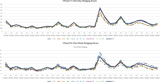
Sub-period Performance Analysis. This figure reports the quarterly average mean absolute errors (MAE) of out-of-sample pricing and hedging performance for each option pricing model. The model ranked first in each sub-period indicates the one with the smallest error. BS refers to the Black and Scholes (1973) model. The A1 model includes an intercept and the strike price as independent variables, while the A2 model includes an intercept, strike price, and squared strike price. The R1 model includes an intercept and moneyness, while the R2 model includes an intercept, moneyness, and squared moneyness. SV and SVJ denote the stochastic volatility model of Bakshi et al. (1997) and the stochastic volatility model with jumps, respectively
The figure shows four graphs arranged in a vertical series. All the graphs display seven lines representing different pricing models. A legend at the bottom identifies the models as “BS”, “A1”, “A2”, “R1”, “R2”, “SV”, and “SVJ”. The top graph is labeled “Panel A: One-Day Out-of-Sample Pricing Errors”. The horizontal axis lists quarterly periods as follows: “A2 – 2015 Q3”, “SVJ – 2015 Q4”, “SVJ – 2016 Q1”, “SVJ – 2016 Q2”, “SVJ – 2016 Q3”, “SVJ – 2016 Q4”, “SVJ – 2017 Q1”, “SVJ – 2017 Q2”, “SVJ – 2017 Q3”, “SVJ – 2017 Q4”, “SVJ – 2018 Q1”, “SVJ – 2018 Q2”, “SVJ – 2018 Q3”, “SVJ – 2018 Q4”, “SVJ – 2019 Q1”, “SVJ – 2019 Q2”, “SVJ – 2019 Q3”, “SVJ – 2019 Q4”, “A2 – 2020 Q1”, “SV – 2020 Q2”, “SV – 2020 Q3”, “SV – 2020 Q4”, “SVJ – 2021 Q1”, “SVJ – 2021 Q2”, “SVJ – 2021 Q3”, “SVJ – 2021 Q4”, “SVJ – 2022 Q1”, “SVJ – 2022 Q2”, “SVJ – 2022 Q3”, and “SVJ – 2022 Q4”. The vertical axis ranges from 0.0 to 0.8 in increments of 0.1 units. Each line shows quarterly pricing error fluctuations, with the model “R2” displaying the highest spikes—particularly near 2017 Q2 and 2021 Q1—and the model “SVJ” consistently producing the lowest errors throughout the period. The second graph is labeled “Panel B: One-Week Out-of-Sample Pricing Errors”. The horizontal axis lists quarterly periods as follows: “A2 – 2015 Q3”, “SVJ – 2015 Q4”, “A1 – 2016 Q1”, “A1 – 2016 Q2”, “SVJ – 2016 Q3”, “SVJ – 2016 Q4”, “SVJ – 2017 Q1”, “BS – 2017 Q2”, “SVJ – 2017 Q3”, “SVJ – 2017 Q4”, “A1 – 2018 Q1”, “SVJ – 2018 Q2”, “SVJ – 2018 Q3”, “A1 – 2018 Q4”, “SVJ – 2019 Q1”, “SVJ – 2019 Q2”, “SVJ – 2019 Q3”, “SVJ – 2019 Q4”, “A1 – 2020 Q1”, “SVJ – 2020 Q2”, “SV – 2020 Q3”, “SVJ – 2020 Q4”, “SVJ – 2021 Q1”, “SVJ – 2021 Q2”, “SVJ – 2021 Q3”, “SVJ – 2021 Q4”, “SVJ – 2022 Q1”, “SVJ – 2022 Q2”, “SVJ – 2022 Q3”, and “SVJ – 2022 Q4”. The vertical axis ranges from 0.0 to 1.6 in increments of 0.2 units. Across the period, the model “R2” exhibits the highest spikes, peaking at 1.4 around 2017 Q2 and approaching 1.2 near 2021 Q2. The models “A1”, “A2”, “BS”, and “SV” show moderate fluctuations between 0.2 and 0.6, with noticeable increases in 2020 Q1–Q2. The model “SVJ” consistently produces the lowest pricing errors, mostly between 0.1 and 0.4, with small rises near 2020 Q1 and 2021 Q3. The third graph is labeled “Panel C: One-Day Hedging Errors”. The horizontal axis lists quarterly periods as follows: “A2 – 2015 Q3”, “A2 – 2015 Q4”, “A2 – 2016 Q1”, “A2 – 2016 Q2”, “A2 – 2016 Q3”, “A2 – 2016 Q4”, “R2 – 2017 Q1”, “A2 – 2017 Q2”, “A2 – 2017 Q3”, “A2 – 2017 Q4”, “A2 – 2018 Q1”, “A2 – 2018 Q2”, “A2 – 2018 Q3”, “A2 – 2018 Q4”, “A2 – 2019 Q1”, “A2 – 2019 Q2”, “A2 – 2019 Q3”, “A2 – 2019 Q4”, “A2 – 2020 Q1”, “A2 – 2020 Q2”, “A2 – 2020 Q3”, “A2 – 2020 Q4”, “A2 – 2021 Q1”, “A2 – 2021 Q2”, “A2 – 2021 Q3”, “A2 – 2021 Q4”, “A2 – 2022 Q1”, “A2 – 2022 Q2”, “A1 – 2022 Q3”, and “A2 – 2022 Q4”. The vertical axis ranges from 0.0 to 0.45 in increments of 0.05 units. A noticeable spike occurs around 2020 Q1, where all models increase sharply, with “R2” and “SVJ” reaching the highest values, slightly above 0.35 and 0.30, respectively. Smaller peaks appear near 2018 Q1, 2019 Q3, and 2021 Q1, where errors rise but stay below 0.25. The models “A1”, “A2”, “BS”, and “SV” fluctuate between 0.05 and 0.20 for most periods. The model “SVJ” shows slightly higher hedging errors relative to others, except outside major spike periods. The bottom graph is labeled “Panel D: One-Week Hedging Errors”. The horizontal axis lists quarterly periods from 2015 Q3 to 2022 Q4, with each period labeled by the model used: “A2 – 2015 Q3”, “A2 – 2015 Q4”, “A2 – 2016 Q1”, “A2 – 2016 Q2”, “A2 – 2016 Q3”, “A2 – 2016 Q4”, “A2 – 2017 Q1”, “A2 – 2017 Q2”, “A2 – 2017 Q3”, “A2 – 2017 Q4”, “A2 – 2018 Q1”, “A2 – 2018 Q2”, “A2 – 2018 Q3”, “A2 – 2018 Q4”, “A2 – 2019 Q1”, “A2 – 2019 Q2”, “A2 – 2019 Q3”, “A2 – 2019 Q4”, “A2 – 2020 Q1”, “A2 – 2020 Q2”, “A2 – 2020 Q3”, “A2 – 2020 Q4”, “A2 – 2021 Q1”, “A2 – 2021 Q2”, “A2 – 2021 Q3”, “A2 – 2021 Q4”, “A2 – 2022 Q1”, “A2 – 2022 Q2”, “A2 – 2022 Q3”, and “A2 – 2022 Q4”. The vertical axis ranges from 0.0 to 0.7 in increments of 0.1 units. Most models show low and stable hedging errors between 0.05 and 0.20 across the sample. A prominent spike occurs around 2020 Q1, where all models rise sharply, with “BS”, “A1”, “A2”, “R1”, “R2”, “SV”, and “SVJ” reaching values between 0.35 and 0.65 before returning to lower levels. Additional smaller peaks occur near 2018 Q1, 2019 Q3, and 2021 Q1, with values remaining below 0.35. Across the sample, “SVJ” and “BS” tend to produce slightly higher hedging errors, while “A1” and “A2” are generally lower except during volatility spikes. Note: All numerical data values are approximated.Sub-period Performance Analysis. This figure reports the quarterly average mean absolute errors (MAE) of out-of-sample pricing and hedging performance for each option pricing model. The model ranked first in each sub-period indicates the one with the smallest error. BS refers to the Black and Scholes (1973) model. The A1 model includes an intercept and the strike price as independent variables, while the A2 model includes an intercept, strike price, and squared strike price. The R1 model includes an intercept and moneyness, while the R2 model includes an intercept, moneyness, and squared moneyness. SV and SVJ denote the stochastic volatility model of Bakshi et al. (1997) and the stochastic volatility model with jumps, respectively
In summary, the robustness checks demonstrate that the SVJ model consistently outperforms others in option pricing across different time horizons and market conditions, while the A2 model provides the most reliable hedging performance. These findings reinforce the main results of this study and highlight the importance of incorporating both stochastic volatility with jumps for pricing accuracy and parsimonious smile specifications for effective hedging.
5. Conclusion
This study investigates the optimal option pricing model in the KOSPI 200 options market under changing market conditions and investor composition. For comparison of in-sample pricing, out-of-sample pricing, and hedging performance, we employed the Black–Scholes (BS) model, the Adjusted Black–Scholes (AHBS) models obtained by regressing implied volatilities on strike and moneyness variables, and more advanced models incorporating stochastic volatility and jumps, namely the SV and SVJ models.
The results show that the SVJ model, which simultaneously accounts for stochastic volatility and jumps, delivers the best performance in both in-sample and out-of-sample pricing. In contrast, in terms of hedging performance, the A2 model—an AHBS specification that includes both strike price and its squared term as independent variables—consistently outperforms all other models. These relative rankings remain stable across forecasting horizons of one, three, five, and seven days, as well as across quarterly subsamples that encompass different market conditions, including the COVID-19 crisis. Furthermore, pairwise statistical tests confirm that the differences in model performance are statistically significant.
The findings also reveal that the dominance of option pricing models is closely related to changes in liquidity and investor structure. In the early stage of the KOSPI 200 options market, when retail investors accounted for the majority of trading and liquidity was abundant, simpler BS-based AHBS models outperformed. In recent years, however, as the share of retail investors has declined sharply and foreign investors have become dominant, mathematically sophisticated models such as the SVJ have shown clear superiority. This underscores the role of market microstructure in shaping the effectiveness of option pricing models.
Moreover, the results are consistent with existing studies on the KOSPI 200 weekly and mini options markets. Taken together, the evidence suggests that the regular, weekly, and mini KOSPI 200 options markets function efficiently as interconnected markets through arbitrage, despite differences in product specifications.
Finally, the divergence between the optimal pricing and hedging models reflects the practical trade-offs faced by market participants. In real trading, practitioners often employ simple AHBS-type models for hedging due to their stability and transparency, while using more sophisticated SVJ-type models for valuation and risk assessment. This dual dominance is thus consistent with the empirical behavior observed in the KOSPI 200 options market.
These empirical patterns also carry practical implications. In markets where institutional investors play a dominant role, adopting stochastic-volatility-with-jumps models can improve pricing precision and risk measurement. Conversely, for routine hedging and portfolio adjustments, parsimonious AHBS specifications may offer greater stability and lower estimation noise. This trade-off suggests that regulators and market participants should consider the evolving investor composition when setting model standards for derivatives valuation and risk management.
The author would like to express deep gratitude to the two anonymous referees and the editor-in-chief for their thoughtful and detailed reviews, which greatly improved the quality of this paper. Any remaining errors are solely the responsibility of the author. This work was supported by the Hankuk University of Foreign Studies Research Fund.
Notes
Key developments include stochastic interest rate frameworks (Amin and Jarrow, 1991, 1992; Rindell, 1995; Ho et al., 1997), stochastic volatility models (Hull and White, 1987; Heston, 1993; Johnson and Shanno, 1987; Melino and Turnbull, 1990; Scott, 1987; Stein and Stein, 1991; Wiggins, 1987), and jump-diffusion or regime-switching models (Merton, 1976; Naik, 1993; Naik and Lee, 1990; Kou, 2002; Kou and Wang, 2004; Jang and Koo, 2024), along with GARCH-type approaches (Duan, 1995; Heston and Nandi, 2000; Duan and Zhang, 2001; Hsieh and Ritchken, 2005).
The AHBS framework was popularized by Dumas et al. (1998) and further analyzed by Li and Pearson (2008a, 2008b), Jackwerth and Rubinstein (2012), and Dixit and Singh (2018).
Comparative evidence includes Bakshi et al. (1997, 2000), Bates (2003), Kim and Kim (2004, 2005), Choi and Ok (2011), Choi et al. (2012), and Kim (2009, 2014a, 2014b, 2017).
See Koo and Kim (2024).
The one-minute KOSPI 200 index and option price data required for model evaluation were purchased from the Korea Exchange (KRX).
It is the condition that ensures option prices satisfy their theoretical upper and lower bounds.
See Hwang et al., (2013).
The KOSPI 200 weekly option market was launched on September 23, 2019. Since it is included in the sample period following the introduction of the KOSPI 200 mini option market, this study employs the same sample as Kim (2025), which analyzes the KOSPI 200 mini options.
The Korea Exchange provides data on KOSPI 200 option trading volume and value by investor type since 1999.
It should be noted, however, that based on MSE, the A1 model consistently outperforms the A2 model across all forecast horizons.
