

Many small and medium manufacturing companies face challenges with global competition due to limited access to advanced machinery and high overhead costs necessary to implement product-mandated line changes. To tackle this challenge, the concept of a distributed digital factory (DDF) has been proposed as compared to a traditional factory (TF).
This research used multiple case studies to identify potential issues and propose and validate solutions using DDF and TF in various manufacturing scenarios to address global challenges like cost reduction, productivity and flexibility to meet uncertain demands. Finally, queuing and simulation models were developed for feasibility analysis on isolated co-located factory environments and DDFs to reduce production lead time or improve customer response. The model identified DDF and TF variables, efficiency and correlations using global balance conditions to measure performance.
This paper theorized and researched four cases to determine manufacturing costs and capacity. DDF saved 9 and 14% as compared to TF in the first and second cases, respectively. Compared to traditional methods, DDF reduced queue time by 22.95 and 26.32% in two distributed factory facilities in the third case. In the fourth case, DDF handled 99% product demand situations and TF 28%.
This paper is the first paper that investigates and researches the specific factors and scenarios through which a DDF setup becomes more efficient, productive and cost-effective through several cases and sensitivity analysis.
Nomenclature
1. Introduction
1.1 Rational behind distributed digital factory (DDF)
In recent decades, the world has moved toward a global manufacturing and assembly supply chain, making businesses more competitive and demanding high-quality products at low costs and shorter response times to meet changing customer needs. Traditional centralized production of entire product lines in one location is struggling to meet these needs. To stay relevant in such competitive markets, staying agile, while delivering quality products, at minimal costs, and short lead times are important factors for any individual company (Leitão, 2009; Zheng et al., 2018). Additionally, in a traditional centralized system which generally follows a fixed layout production floor, extra time and expense are mandated to switch to producing new products. If any disruptions affect this TF production line, the maintenance costs, and production time loss will ultimately detrimentally affect their expected production quantity (Tariq et al., 2023; Wang et al., 2021; Zhu, Dhokia, Nassehi, & Newman, 2013).
To meet these needs of today, a DDF is proposed, which connects multiple factories from geographically dispersed locations all over a country or the world to make the production system more flexible, smart and customized (Matt, Rauch, & Dallasega, 2015). Many researchers have tried to demonstrate a DDF’s scope, challenges and opportunities (Matt et al., 2015; Tariq et al., 2023; Wang et al., 2021; Zheng et al., 2018; Zhu et al., 2013). The DDF model can combine subtractive and additive manufacturing to produce parts in locations with resources to quickly manufacture goods. Through AM and SM integration using a DDF, some products can be made using SM and some parts using AM, then assembled to complete the product (Settineri, Priarone, Di Lorenzo, & Ingarao, 2020). Jacob Lohmer et al. discussed that many researchers have been working on production planning and scheduling for different DDF scenarios (Lohmer & Lasch, 2021). One TF factory handles demand, making production planning difficult based on customer and product specifications. Multiple case studies show that DDF spreads demand across multiple factories, eliminating bottlenecks and production planning issues. Each DDF factory was able to meet customer demands with minimal time and capacity.
1.2 Leveraging industry 4.0 for DDF
The advancements in information technology have led to the development of different technologies, such as the Internet of Things (IoT) and the use of cloud computing. Other current research areas like Cyber-Physical Systems (CPS), Virtual and Augmented Reality (VR & AR), analytical models, and digital twins, assist industries in maintaining material bills, production planning, and facility location and enable the advancement of aggregate and flexible manufacturing systems (Bartsch, Pettke, Hübert, Lakämper, & Lange, 2021; Morgan, Halton, Qiao, & Breslin, 2021; Rejeb, Simske, Rejeb, Treiblmaier, & Zailani, 2020; Zhou, Zhou, Wang, & Zang, 2019). As a result, a DDF virtually connects many small and medium factories and delivers customized products within their specifications and expected lead time to suit a diverse range of customer needs. In addition, advancements in technology enable real-time monitoring, optimizing scheduling, and process modeling, which can enable cost-saving products and higher utilization of capital equipment (Tariq et al., 2023; Tofail et al., 2018). Wang, Wan, Li, and Zhang (2016) have used wireless networks, and cloud computing to incorporate Industry 4.0 in a traditional production line, associated machines and some conveyors. With the help of a control engineering-driven open and closed feedback control system, the main technical features with their outcomes have been demonstrated and are helpful to the design and implementation of a viable DDF (Mourtzis, 2020).
1.3 Related studies
Adoption of mixed methods research has become rather popular in manufacturing and industrial engineering studies in recent years since it provides a thorough framework for exploring challenging systems (Creswell & Creswell, 2018; Garrido-Moreno, Martín-Rojas, & García-Morales, 2024). Combining qualitative case study analyses with quantitative methods, including mathematical modeling and simulation, will help researchers to present a more complete picture of manufacturing paradigms. Reliable and significant insights, however, depend on methodical rigor being ensured. Using accepted scientific research techniques, a well-organized mixed methods approach increases the validity and applicability of results. Following mixed methods research guidelines, such as those suggested by (Creswell & Creswell, 2018; Venkatesh, Brown, & Bala, 2013), methodically combines empirical data, theoretical modeling, and case-based validation, thereby enhancing the credibility of the study.
Though mixed methods research is popular in manufacturing and industrial engineering studies due to its ability to combine qualitative and quantitative insights, this paper employs a multiple-case study approach. While simulation models are incorporated to support case-based insights, the primary emphasis remains on empirical, quantitative investigation rather than a fully integrated mixed methods approach (Baxter & Jack, 2015; Yin, 2018). This work ensures a strong and scientifically sound approach by using a multi-case study methodology together with time and financial analysis to investigate the feasibility of DDFs over TFs. TFs and DDFs were compared in this way using the case-based study in response to the necessity to look at real-world manufacturing challenges experienced by SMEs in an ever evolving and future looking manufacturing paradigm. Unlike mixed methods research, a multiple-case approach allows for the fine-grained analysis into how various manufacturing setups perform under different conditions, considering the unique challenges and characteristics specific to each manufacturing environment (Ridder, 2017). Additionally, multiple-case studies allow for replication logic, which increases generalizability and reliability in different industrial environments (Eisenhardt and Graebner, 2007; Eisenhardt, 1989). By adopting this multiple case study approach (Ranta, Aarikka-Stenroos, & Väisänen, 2021; Rashid, Rashid, Warraich, Sabir, & Waseem, 2019), this study not only strengthens analytical generalizability but also ensures practical relevance by evaluating the real-world feasibility of TFs and DDFs under dynamic manufacturing conditions.
Although DDF can integrate small and medium industries to produce a diverse range of products using both AM and SM, it is necessary to understand the financial feasibility and other capabilities needed to meet customer expectations like low cost, desired quality, and low response times etc. (Hodek & Floerchinger, 2009). In practice, only 5–10% of business or proposed projects come to limelight (Dikareva & Voytolovskiy, 2016). Research needed in this regard includes economic analysis of manufacturing, assembly, production, and transportation bottlenecks that will strengthen business proposals. Project feasibility is determined by net present value (NPV), payback period, internal rate of return (IRR), capital budgeting, simulation, and modeling. Comparison of project costs requires analysis. Lower costs make projects more profitable and attractive investments. The internal rate of return helped Ira Altman et al. make US biopower feasibility analysis financial decisions. Projects were suitable in three case studies, but case three had the highest internal rate of return and was the most cost-effective (Altman, Johnson, Badger, & Orr, 2007). Merzi and Daryanto (2018) used Payback Period, Return on Investment, NPV, NPV Index, Discounted Payback Period, and internal rate of return (IRR) to show the feasibility analysis of different options like the first alternative, which uses the government selling price with subsidy, and the second alternative based on purely commercial pricing for the Perusahaan gas negara project. Based upon the different capital budgeting indicators, the second option was found to be feasible, while the first was not.
To analyze the capability of any DDF over TF, simulation models are typically used when it is not feasible and highly complex to build an analytical solution to a given topic. Given the dynamic nature of these intricate systems and the absence of specialized analytical models for design, analysis, and optimization, simulation is a viable appropriate approach to virtualize the environment, to understand and propose solutions to potential bottlenecks (Kikolski, 2016, 2017; Ma & Qu, 2014). The complexity of these systems necessitates the use of simulations to study these models, as mathematical tools are insufficient due to the proposed environments’ complexity wherein this simulation modeling and analysis is used to gain a deep understanding of these intricate systems (Carl May, Nestroy, Overbeck, & Lanza, 2024). They allow for conducting trials of innovative operational or resource policies, ideas, or sub-systems before physical implementation (Chung, 2003), with minimal capital and resource investments. These complex models also allow for information and knowledge gathering without causing disruption to a real manufacturing environment (Mourtzis, Doukas, & Bernidaki, 2014).
Queuing theory studies models that predict the behavior of a manufacturing process that manages intermittent demands at a production workstation. Using this paradigm, people can quickly determine the best course of action for a factory or group of factories’ waiting list, increasing productivity. Engineers have used queuing theory findings to illustrate the links between important metrics like cycle time, machine utilization, inter-arrival time statistics, and service (Meisling, 1958; Sarkar, Mukhopadhyay, & Ghosh, 2015). Applications of queuing theory to manufacturing industries with assembly processes that are being researched worldwide aim to model the assembly process in a manufacturing facility using an appropriate analytical framework. A company’s standard data can be compared to this model’s significant variables and metrics. Any such queuing model must be evaluated to determine its efficacy in recommending ways to improve workstation performance and efficiency (Shafeek and Muhammed Marsudi, 2014).
Despite investigations into various manufacturing environments, DDFs’ financial feasibility, production capacity, and operational success compared to TFs are unknown. Selection of TF system technologies and scheduling of manufacturing processes currently dominate research in this area. DDF efficiency depends on financial and operational factors like response times, output, and equipment availability which can be optimized to meet a range of customer demands. Simulation or analytical models coupled with queuing theory have been used in other manufacturing environments, but DDFs, particularly AM and SM process integration across multiple sites, have not been extensively studied. This paper expands on these challenges of manufacturing systems, simulation, queuing theory, and financial feasibility analysis and their integration into a holistic solution to demonstrate DDF’s feasibility with multiple case studies over traditional factories. Two scenarios were analyzed to determine DDFs’ financial viability over TFs. Additionally, two more cases were investigated to demonstrate DDF’s ability to quickly meet variable new product manufacturing and repair demands. This paper compares DDFs to traditional factories using both a queuing model and an AM-SM simulation model, assessing their performance using ARENA simulation software. Finally, a sensitivity analysis examined DDF and TF performance under geographical arbitrage, demand types, and quantity variation, all of which are critical variables to the understanding and deployment of DDFs and promoting further research in this area.
2. Research methods
Many research disciplines, including business, social science, and information technology, make extensive use of case study research (Genzorova, Corejova, & Stalmasekova, 2019; Moreno et al., 2017; Telukdarie & Sishi, 2020; Vennesson, 2008; Wittbrodt, Laureto, Tymrak, & Pearce, 2015). Multiple case analysis yields detailed findings compared to single case analysis, as it benefits from the power of replication logic (Hollweck, 2015). A multiple case study analysis enables the examination of data within each individual situation as well as a comparative assessment across different situations. This approach can be employed to predict either differing outcomes based on anticipated factors or comparable outcomes across the studies. Furthermore, employing many cases enables researchers to conduct cross-case comparisons, facilitating a comprehensive understanding of the distinctions and similarities across various situations (Baxter & Jack, 2015; Eisenhardt & Graebner, 2007; Hollweck, 2015; Vannoni, 2015; Zangiacomi, Pessot, Fornasiero, Bertetti, & Sacco, 2020). When conducting multiple case analyses, there is no definitive answer on the exact number of examples required. However, it is generally recommended to have between 4 and 10 cases to facilitate the emergence of both comparable and contrasting outcomes (Seawright & Gerring, 2008). In this paper, four different cases of TF and DDF are presented.
2.1 Theoretical background of single line multistage model of TF
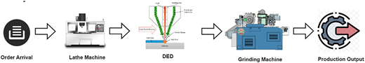
Product-driven or sequential plants have a single line with sequential machines on their production floor. This production system handles one order type. When customers order multiple products at once, it can take a long time to adjust the TF environment to start producing a new product on the same line. This reduces production and may increase waiting times for those products. Figure 1 shows TF with lathes, DEDs, and grinding machines and the system’s order-taking process. The system serves orders sequentially with servers. Servers are treated as machines and peripherals, and the product leaves the production line after all services are completed. A single-line multistage model was created to analyze and manage the above system:
The following standard terminology and notation is used henceforth:
The average arrival rate (λ) is the expected number of arrivals per unit of time.
µ measures the average overall system service completion rate for each server, measured in parts per unit of time.
Pn indicates the likelihood of accurately having n queueing system components.
Ls is the estimated number of pieces in a queueing system.
Ws is the expected wait time for customers in the system.
Lq represents the expected queue length.
Wq represents the expected wait time for customers.
ρ is the equipment utilization factor.
k represents stage count.
The number of parallel lines is m.
The utilization factor, or the fraction of time that servers are busy, is:
The probability of having a specific number, n, clients in the system may be calculated using the following expression:
The anticipated number of clients in the queue can be determined by:
Expected number of clients in the system:
The mean duration of client wait time in the queue:
Anticipated customer wait time in the queue:
2.2 Theoretical background of multi-line multistage model in DDF
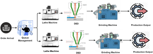
Like TFs, DDF connects factories with one line of sequential machines. Multi-order processing using different manufacturing lines is possible with this system. Customer orders determine which factory production line starts with scheduling software. This factory doesn’t need to modify its production lines for new or different products because different systems can handle different orders. So, line modifications don’t reduce production. DDF has lathes, direct energy deposition (DED), and grinding machines connecting two companies’ manufacturing lines (Figure 2). For system analysis and management, Figure 2 shows a multi-line multistage model.
The utilization factor, often known as the fraction of time, that servers are busy, is:
The probability of having a specific number, n, of clients in the system may be calculated using the following formula:
The anticipated number of clients in the queue can be determined by:
Expected number of clients in the system:
The mean duration of client wait time in the queue:
Anticipated customer wait time in the queue:
2.3 ARENA simulation model description
Figure 3 illustrates how models simulate every TF manufacturing step. The illustration shows that ARENA software entities must be organized and categorized from left to right. All six counters in this case study were simulated using ARENA software © 2020 by Rockwell Automation, Inc. version 16.10.0002. Three dependent sequential processes occurred between the first and last counters for part arrival and disposal. To adapt to changing processing times, an assign module was added. The ARENA manufacturing system simulates 1,000 work hours.

This paper utilizes case studies to examine the use of DDF in business contexts from a commercial standpoint. The diverse case technique was employed to choose cases, ensuring that a wide range of relevant situations for different applications were considered, thus guaranteeing the necessary variation that would mimic real life usage scenarios. A discussion of the specifics of each of the five cases is included in the following sections.
3. Case formulation
Many operational and financial elements, including the stability of demand, the variety of products, and the capacity for production, greatly affect the practicality of DDF as compared to TF. Examining the feasibility of financial and production capacity in a sequential product layout helps this paper determine whether DDF is suitable in four separate cases.
Case Study A: Financial feasibility analysis of DDF over TF in a sequential product layout plant where demand is single-type repaired parts.
Case Study B: Financial feasibility analysis of DDF over TF in a sequential product layout plant where demand is uncertain, and the product line exhibits significant variety.
Case Study C: Production capacity feasibility analysis of DDF over TF in a sequential product layout plant where demand is single-type repaired parts using ARENA Software
Case Study D: Production capacity feasibility analysis of DDF over TF in a sequential product layout plant where demand is uncertain, and the product line exhibits significant variety by ARENA Software
Examining scenarios with single-type repaired parts against uncertain demand with high product variety helps this study show when DDF offers a competitive advantage over TF. While Case Studies C and D use ARENA software to evaluate manufacturing capacity feasibility, Case Studies A and B evaluate financial feasibility. By means of these analyses, the aim of this work is to identify the particular conditions under which DDF is a more viable substitute for TF, so offering a data-driven approach to decision-making in contemporary manufacturing.
3.1 Case study A: financial feasibility analysis of DDF over TF in a sequential product layout plant where demand is single-type repaired parts.
This case study assumes that a manufacturer has received some orders to repair one type of expensive die. To repair this die, the company needs some machines, but the repair can be completed using either DDF or TF. For deciding between TF and DDF, the cost analysis tool helps as a financial indicator to decide which incurs less cost to make this product. Assumptions in this case include:
Demand is deterministic.
The machine time of various products in the two systems is constant and the same.
There is no breakdown of any equipment in these two production lines.
The Factory is established as sequential or product layout.
Material cost is the same for both TF and DDF factories.
The formula for calculating payback period and production cost (Sinambela, Darmawan, & Gardi, 2022; Garrison, Noreen, Brewer, & McGowan, 2010) is
Based on the above formula, the manufacturing cost in each factory was calculated and compared to determine the contribution margin in each factory. In addition, the payback period as part of manufacturing overhead calculations was also estimated and included in the analyses. The detailed calculations for labor cost, material cost and manufacturing overhead are provided in a downloadable/editable file through the GitHub repository (Ahmmed, 2024).
3.1.1 TF environment
A well-recognized die manufacturing company is situated in New York, USA. The factory consists of six primary cells for repairing forged dies. In that factory, the labor cost per year varied depending upon the experience of labor and the sectors in which they worked (Salary.com, 2024; Talent.com, 2024; Ziprecruiter, 2024). There were 302 laborers directly involved in producing the products and it cost $7,670.09 per die (Ahmmed, 2024). The material cost per unit of forged die was $23,490.00, which is detailed in Table 2, and the manufacturing overhead cost was $5,655.62 per die. The manufacturing plant was assumed to be installed this year at a cost of $33,887,746 with a 5-year payback period (Ahmmed, 2024).
Resource information on various factories in DDF
| Machine name | |||||||||
|---|---|---|---|---|---|---|---|---|---|
| Factory 01 | Machine 01 | Machine 02 | Machine 03 | Machine 04 | Machine 05 | Machine 06 | Machine 07 | Machine 08 | Machine 09 |
| Factory 02 | Machine 02 | Machine 03 | Machine 05 | Machine 07 | Machine 08 | Machine 09 | |||
| Factory 03 | Machine 01 | Machine 03 | Machine 05 | Machine 07 | Machine 08 | Machine 09 | |||
Source(s): Authors’ own work
3.1.2 DDF environment
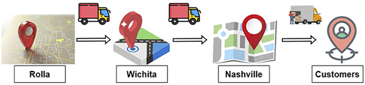
DDF facilities were in Rolla, Missouri, Wichita, Kansas, and Nashville, Tennessee. Because of cheaper land and resources, factories were built. With lower land prices per acre than New York, Rolla, Wichita, and Nashville had lower initial investments than the factory. DDF installation cost $29,445,034 this year. Like TF, 302 workers directly produced products. Since those states had cheaper hourly labor, (Salary.com, 2024; Talent.com, 2024; Ziprecruiter, 2024), cost per die: $6,232.72. Since forged die material cost was $23,490.00 like TF, manufacturing overhead cost was $3,598.08 per die. With a 5-year payback, the manufacturing plant was installed this year at $29,516,026 to produce 2,000 dies per year. Because of DDF, the product must be moved between factories for die repair operations. This product was transported as shown in Figure 4. Considering Figure 4, transportation costs are taken from freight run as $274 (Freight.com, 2024).
3.2 Case study B: financial feasibility analysis of DDF over TF in a sequential product layout plant where demand is uncertain, and the product line exhibits significant variety.
In this case, factories are in the same areas as considered in the previous case, but the difference is that the order stream includes different types of products that make the demand uncertain. This case has been analyzed taking into consideration the need to handle varieties in demand and thereby demonstrating capability of DDFs and TFs meeting these uncertain demands. In this scenario, multiple dies from different customers are placed in the order queue for repair. To repair those dies, the company needs some machines but either DDF or TF can be used for these purposes. For deciding between TF and DDF, the cost analysis tool helps as financial indicator to decide which incurs less cost to make this product. Assumptions are given below:
Demand is deterministic.
The machine time of various products in the two systems is constant and the same.
There is no breakdown in the two systems.
Switching time is constant among all products.
After completing a minimum quantity of a product, the next demand for another product must be met; in this way, whole production moves first to last in an acyclic order until the end of production.
Factory is established as sequential or product layout.
Material cost is the same for both TF and DDF systems.
3.2.1 TF environment
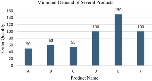
Like the previous case, a well-known die manufacturing company is in New York. Figure 5 shows its single-line, product-driven production line in this scenario. Six orders (labeled “A” to “F” in Table 1) have been received by the factory with a minimum delivery time of 7,460 hours. TF floors are sequential; therefore, every product must pass through all cells on the product line, regardless of operations. If a TF produces “A”, it must fill the minimum quantity and take the time to fulfill the minimum order quantity of “B” and then “C” and so on until it reaches 7,460 hours. Table 4 shows machine times for distinct items. The shapes and sizes of the dies in this manufacturing process and the activities needed to meet each requirement affect how long each machine takes to make each product.
Time spent for value addition by several machines for specific products
| Product name | Machine 01 (hours) | Machine 02 (Hours) | Machine 03 (Hours) | Machine 04 (Hours) | Machine 05 (Hours) | Machine 06 (Hours) | Machine 07 (Hours) | Machine 08 (Hours) | Machine 09 (Hours) |
|---|---|---|---|---|---|---|---|---|---|
| A | 0.02 | 0.03 | 0.04 | 0.02 | 0.026 | 0.1 | 0.026 | 0.04 | 0.02 |
| B | 0.04 | 0 | 0.022 | 0.04 | 0 | 0.04 | 0.04 | 0 | 0.08 |
| C | 0 | 0.024 | 0.04 | 0 | 0.04 | 0 | 0.02 | 0 | 0.026 |
| D | 0.06 | 0.007 | 0.3 | 0.4 | 0 | 0 | 0.03 | 0 | 0.01 |
| E | 0 | 0 | 0 | 0 | 0.02 | 0.05 | 0.06 | 0.07 | |
| F | 0.05 | 0 | 0.006 | 0 | 0 | 0 | 0.02 | 0.02 | 0.05 |
Source(s): Authors’ own work
Input data for the ARENA model
| Module name | Distribution with data |
|---|---|
| Parts Arrival | Random (exponential distribution) (λ = 5) |
| Decide | 2-way by chance (33%) |
| Delay | Triangular (18,22,24) |
| Server 01(Shaper/Lathe) | Triangular (4,6,8) |
| Server 02 DED/laser powder bed fusion (LPBF) | Triangular (4,6,8) |
| Server 03(Grinding Machine) | Triangular (4,6,8) |
Source(s): Authors’ own work
For instance, each product must run from machine 1 to machine 9 to finish. After the desired quantity of “A” is completed, the line is shifted to another product, and so on. Switching from one product to another requires time in the factory line to accommodate the adjustments for the next product, which will follow sequential operations from machine 1–9 till product F. Both systems’ change overtime is expected to be 16 hours. So, TF will move from product to product till completion. Customers need each product at least as shown in Figure 6.
In this scenario, the machine time of a specific product and minimum number of orders and time were the same as TF. Table 2 shows the equipment available in various factories which are now connected under a DDF.
The DDF can send items A to factory 01, E to factory 02, and F to factory 03 simultaneously, depending on machining requirements, unlike a TF. After a period, these products are transported to other factories based on machine availability and machining needs. Table 3 shows product shipping time between DDF factories.
Transportation time among several factories in a DDF
| Factory 01(Hours) | Factory 02(Hours) | Factory 03 (hours) | |
|---|---|---|---|
| Factory 01 | 0 | 48 | 72 |
| Factory 02 | 48 | 0 | 24 |
| Factory 03 | 72 | 24 | 0 |
Source(s): Freight.com (2024). Authors’ own work
3.2.2 Assumptions
Machining time for various products between DDF and TF is constant.
Material costs are the same in both DDF and TF.
The changeover time is fixed.
There is no breakdown in the equipment in the two production lines.
Transportation time is computed for the DDF and not for the TF.
After Completing a cycle for a product, the demand for the next product must be met, which drives the whole production first to last in an acyclic order among various factories.
3.3 Case study C: production capacity feasibility analysis of DDF over TF in a sequential product layout plant where demand is single-type repaired parts by ARENA software
Data Analysis – Both TFs and DDFs were simulated using ARENA software with hypothetical data. The study included sequential processes, types, processing times, production line capacity, and other relevant data. Table 4 shows the assumed data and probability distributions for this comparison. Time taken by modules like delays and servers/machines is triangular, with left-value representing minimum time, middle value-median time, and right-value highest time.
3.3.1 Model verification and validation
Credible models require evaluations of computer programs, test runs, statistics, and validation activities. To assess sample path trajectories’ viability and validity, simulations were run. Visual simulators like ARENA verify program logic fidelity using code outputs and visuals. To accurately simulate a production line, this simulation model uses several inputs as deterministic variables. By adjusting these values and testing the model, robustness can be assessed. To estimate stochastic confidence in the model’s prediction, model validation replications were estimated. This model had 50 replicates. Simulations showed that the half-width value for various facilities ranged from 0.5 to 0.9, indicating that the mean output of production line equipment is precise and consistent. In 95% of repeated trials, the true mean should be within the interval sample mean ± half width. The lower variability of half-width values indicated better control or stability of the system (Buist et al., 2005). A good simulation replication pattern, as determined here, allows for the generation of statistically relevant data from simulation runs while minimizing computational costs and time and ultimately minimizing real-world processing costs. Traditional factories’ demand-responsive production lines depend on configuration. The same production line can make or repair new parts to finish products. Rearranging production lines for each product can increase manufacturing lead times. To demonstrate DDF’s TF advantages, the suggested comparative model examines part repair and new product development orders. Both systems assume:
Demand follows exponential distribution.
Triangular distribution is employed for turning, drilling, and finishing.
Facilities meet 100% reliability standards for both systems.
Classified Traditional Factory as a single-channel, multi-stage model.
Viewed DDF as a dual-channel, multi-stage mechanism.
Triangular distribution involves transporting raw materials or parts to the next level of production without adding value.
33.0% of demand is for production-specific items, while the rest require general requirements. The simulation lasts 1,000 hours.
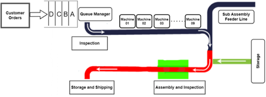
DDF factories share facilities. Mom factories have deciders or workshop schedulers. However, another factory exists elsewhere. ARENA’s delay module requires transporting these factories’ products. Figure 7 shows the design window screenshot and connected boxes of proposed model entities. Delivery, lathe/shaper, DED/LPBF, grinding, and disposal are factory operations in this simulation. After receiving many orders, job schedulers choose which factories to send orders to and in what order to make the product. Capital equipment squares perform these tasks and operations as needed.
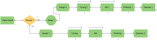
Figure 8 illustrates the manufacturing process scenario following the simulation of a DDF system. Based on the product specifications, availability of production lines, and reaction time, the orders are allocated to various manufacturing lines located in different geographic locations but connected digitally.
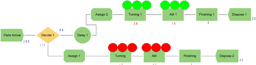
Queue conditions after simulation in DDF where red and green dots are different parts that are being worked in the different production lines of the DDF. Source: Authors’ own work
Queue conditions after simulation in DDF where red and green dots are different parts that are being worked in the different production lines of the DDF. Source: Authors’ own work
3.4 Case study D: production capacity feasibility analysis of DDF over TF in a sequential product layout plant where demand is uncertain, and the product line exhibits significant variety by ARENA software
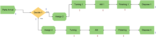
DDF runs two factories in different locations with the same amenities and virtual connections. Mother companies have a decision-maker or workshop scheduler, while other factories are elsewhere. Schedulers assign product orders to manufacturing lines when multiple orders enter the DDF. The procedure was built and executed using ARENA simulation. Figure 9’s design window snapshot shows the proposed model’s entities’ relationships as connected boxes. Five parties make up this simulation’s factories: order arrival, lathe/shaper machine, DED/LPBF, grinding, and disposal.
4. Results and discussion
4.1 Case study A
After calculating the total costs related to the manufacturing, a summary of the cost analysis between the traditional system and the distributed factory is given in Table 5 and 6.
Cost analysis of DDF and TF
| Manufacturing system | Cost for manufacturing of single die |
|---|---|
| DDF | $36546.79 |
| TF | $40204.49 |
| DDF shows 9% cost saving than TF | |
Source(s): Authors’ own work
Cost comparison between DDF and TF
| DDF | TF | ||||
|---|---|---|---|---|---|
| A. Operational costs | $33320.79 | A. Operational costs | $36815.71 | ||
| Labor | $6232.72 | Labor | $7670.09 | ||
| Material | $23490.00 | Material | $23490.00 | ||
| Manufacturing Overhead | $3598.08 | Manufacturing Overhead | $5655.62 | ||
| B. Transportation cost | $274 | ||||
| C. Initial Plant Investment Recovery Cost | $2,952 | B. Initial Plant Investment Recovery cost | $3,389 | ||
| D. Subtotal of Costs (A + B + C) | $36546.79 | E. Subtotal of Costs (A + B) | $40204.49 | ||
Source(s): Authors’ own work
Tables 5 and 6 show that a DDF saves 9% of production costs while meeting product and customer needs. Besides, it takes longer than the traditional plant because the same product must be transported from one location to another for processing, which took 3 days in this case (Freight.com, 2024) as shown in Figure 10 assuming the normal production time is the same in both factories. Due to their geographic locations, DDFs need to transport products across locations, while TFs do not.
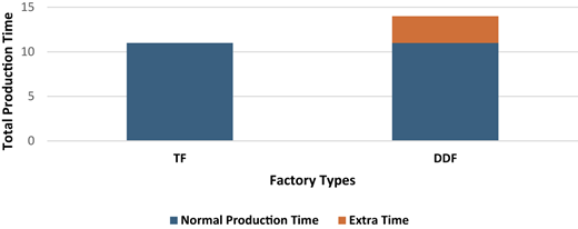
Having determined the additional time, it can be concluded that the DDF costs less to repair the product, while it only added 3 days to this die’s repair and remanufacture and provides a viable alternative for discerning customers. While this adds a time penalty to the DDF-repaired product, it is compensated for by the economic advantage it provides.
4.2 Case study B
After computing this entire stream of orders in Excel, individual cost comparison and capacity analysis between DDF and TF are given below in Table 7.
Cost saving and capacity analysis between DDF and TF
| DDF | TF | Cost saving in DDF (%) | |
|---|---|---|---|
| Product name | Production capacity (Number) | ||
| A | 2,400 | 1,500 | 13 |
| B | 9,600 | 600 | 13.4 |
| C | 135,412 | 5,500 | 15 |
| D | 4,200 | 2,500 | 15.9 |
| E | 9,250 | 2,500 | 15.2 |
| F | 30,224 | 7,551 | 14.3 |
Source(s): Authors’ own work
From Table 8, the distributed factory is again found to be the more economical option as it saves 14.4% of the cost on average, which ultimately aided the overall profit margin. From there, it can be concluded that DDF can handle varieties in demand with significant cost savings by connecting multiple factories that can handle a greater number of uncertain demands than TF.
Overall cost analysis
| DDF | TF | ||||
|---|---|---|---|---|---|
| A. Operational Costs | $20529.56 | A. Operational Costs | $36815.71 | ||
| Labor | $151.53 | Labor | $761.26 | ||
| Material | $20332.86 | Material | $20332.86 | ||
| Manufacturing Overhead | $45.17 | Manufacturing Overhead | $561.32 | ||
| B. Transportation Cost | $274 | ||||
| C. Initial Plant Investment Recovery Cost | $20803.56 | B. Initial Plant Investment Recovery cost | $2,642 | ||
| D. Subtotal of Costs (A + B + C) | $419212468.05 | E. Subtotal of Costs (A + B) | $489627401.49 | ||
Source(s): Authors’ own work
4.3 Case study C
After completion of simulation of DDF and TF, the data shown in Figure 11 illustrates that in TFs, the value-added time per part is 18.239 hours, and there is no non-value-added time because the parts do not have to be transported to different geographic locations unlike in a DDF.
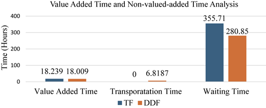
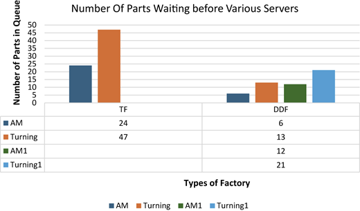
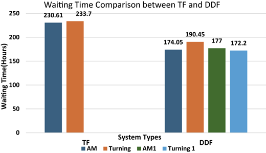
Conversely, each part has a wait time of 355.71 hours, with no transfer time or any other additional time required. Furthermore, Figure 13 demonstrates that there are currently 24 units awaiting service at AM, while 47 units are in queue at turning. Moreover, the average queue time for AM is 230.61 hours, while for Turning it is approximately 233.70 hours.
Number of parts in queue after running simulation of TF and DDF. Source: Authors’ own work
Number of parts in queue after running simulation of TF and DDF. Source: Authors’ own work
According to Figure 11, DDF estimates that the valued added time per part is 18.009 hours, like the TF, and there is no non-valued-added time like transportation. The wait time for parts dropped to 280.85 hours, and it took 6.8187 hours to transfer the product from the parent company to a different company to finish DDF operations. Figure 13 shows 12 units in the AM processing queue and 21 in the Turning queue. Figure 12 also indicates that the AM queue time is 177.69 hours, 22.95% lower than the TF queue time for its AM operations; AM.1 is 174.05 hours; and Turning and Turning.1 are 172.20 and 190.45 hours, 26.32% lower than the TF queue time in Turning.
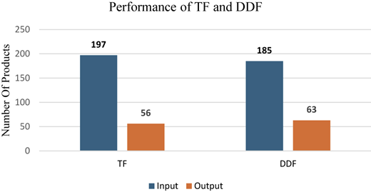
So, Figure 14 shows that the cumulative orders are around 197 units. However, capacity and schedule constraints limit TF production to 56 pieces. Although DDF receives 185 orders, its output is still much higher than TF’s, estimated at 63 units.
In conclusion, DDF performs better than TF for repair products regardless of order quantity or order type, even though we must physically move the products between factories. Reducing or eliminating production changes in DDF improves production efficiency and reduces transportation time.
4.4 Case study D
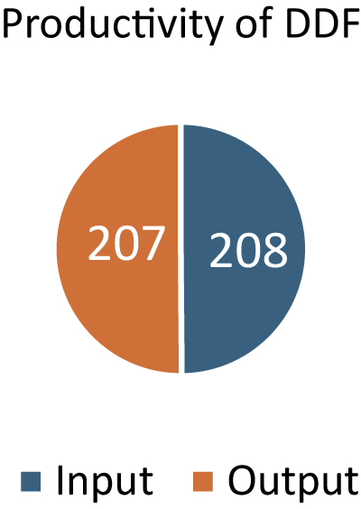
After completion of simulation of DDF and TF, Figure 15 indicates that the suggested DDF can handle different demands by connecting numerous factories. The order was for 208 units based on the demand probability distribution, and after completing different operations by their product variation in separate factories, it produced 207 units using their capacities.
Finally, Figure 16 shows how TF and DDF handle repair and new product development. The line curve shows that DDF handles more product variety orders than TFs. Both methods initially function similarly when production time and product variety are low. When product variety and manufacturing time increase though, DDF vastly outperforms TF. When various product development orders come in, DDF outperforms the other system because it connects multiple factories to manage demand and customer needs.
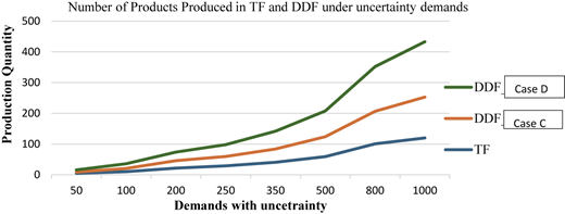
Comparison of repairing parts and new product development performance by DDF and TF as simulated through the ARENA Software. Source: Authors’ own work
Comparison of repairing parts and new product development performance by DDF and TF as simulated through the ARENA Software. Source: Authors’ own work
5. Sensitivity analysis
Evaluating how changes in important operational factors affect the performance of DDF and TF depends mostly on sensitivity analysis. This study offers an understanding of the adaptability and efficiency of both manufacturing models under several conditions considering the uncertainties in manufacturing demand, supply chain fluctuations, and production constraints. This work attempts to find the most resilient and economical manufacturing technique by knowing how sensitive each system is to change in order volume, product variety, and capacity utilization.
5.1 Performance analysis of DDF and TF considering order uncertainty
5.1.1 Sensitivity treatment
Arena was used to build a simulation model to investigate how uncertainty in orders influences TF and DDF performance. Two DDF factories were modeled; each needing a triangular travel time of sixteen, eighteen, and twenty hours. The TF stayed at one fixed, central location. Differentiating the distribution levels of repair orders at 10%, 25%, 50%, 66%, 75%, and 90% introduced order uncertainty. This allowed for balanced assessment of low, moderate, and high variability conditions.
5.1.2 Analysis of DDF and TF considering order uncertainty
As depicted in Figure 17, DDF exhibits superior performance when handling higher order variability, more than around 65% due to its decentralized nature, which in turn allowed for flexible demand management. However, when order uncertainty is low, below 65%, TF demonstrates better performance, as it eliminates inter-facility transportation delays.
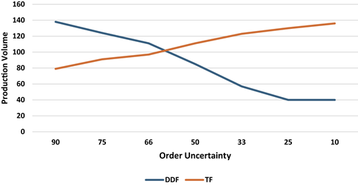
Performance Analysis of DDF and TF considering order uncertainty. Source: Authors’ own work
Performance Analysis of DDF and TF considering order uncertainty. Source: Authors’ own work
DDF boosts production independent of any logistical challenges it may create. By contrast, TF’s production centralization is ineffective in this regard. On high-order uncertainty, however, production losses arise since TF’s rigid structure makes it unable to accommodate demand fluctuations. This implies that TF is more efficient in circumstances of constant demand, while DDF excels in those of uncertain demand.
5.2 Performance Analysis of DDF and TF considering geographical arbitrage
5.2.1 Geographic and transportation-based sensitivity of DDFs and TFs
This sensitivity analysis evaluates how geographical distance between DDF factories influences performance. Four DDF models were simulated with two factories each, maintaining a fixed 25% order variability across all cases. The triangular transportation time distributions were:
Model 1: (1, 1.5, 2) hours
Model 2: (8, 10, 12) hours
Model 3: (12, 14, 16) hours
Model 4: (16, 18, 20) hours
TF was modeled as a single centralized factory with no inter-facility transport. Performance was evaluated based on order fulfillment time, transportation delays, and production efficiency.
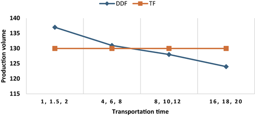
5.2.2 Analysis of DDF and TF considering geographical arbitrage
The four DDF models have two factories and triangular transportation times. All factories have 25% order variety and the same repair order distribution. Figure 18 shows that a TF performs worse than the closely located DDF (1, 1.5, 2) factory due to 25% variety orders. Because demand is predictable, transportation duration does not affect performance. As transportation time increases, DDF models perform worse, as indicated by the 3rd and 4th models which perform worse than TF. As factories get farther apart, performance may decline, but the closest DDF model may still benefit from product variety it can accommodate.
Performance analysis of DDF and TF considering geographical arbitrage. Source: Authors’ own work
Performance analysis of DDF and TF considering geographical arbitrage. Source: Authors’ own work
5.3 Performance analysis of DDF and TF considering order uncertainty and geographical arbitrage
5.3.1 Geographic and transportation-based sensitivity of DDF’s and TFs:
Arena was used to build a simulation model to investigate how DDF and TF performance suffers with order uncertainty. Three DDF manufacturers (DDF1, DDF2, DDF3) were modeled with varying transportation times to evaluate the combined effects of order uncertainty and geographical arbitrage:
DDF1: (2, 1, 1.5) hours
DDF2: 12, 10, 8 hours
DDF3: (16, 18, 20) hours
TF is in one location. Performance measures including order completion time, production delay rate, and system utilization were recorded; the order variability was set at 25%, 50%, and 75%.
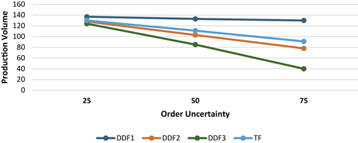
5.3.2 Analysis of DDF and TF considering order uncertainty and geographical arbitrage
While TF is fixed in a specific location, transportation time between DDF1, DDF2, and DDF3 factories is triangular (1, 1.5, 2), (8, 10, 12), and (16, 18, 20). All factories distribute repair orders evenly, with 25%, 50%, and 75% order variety. From Figure 19, DDF is better than TF for order uncertainty and closely located factories, but TF is viable if the factories in the DDF are farther apart. Traveling between factories to repair products creates nonvalue-added time while explaining these results.
Performance analysis of DDF and TF considering order uncertainty and geographical arbitrage. Source: Authors’ own work
Performance analysis of DDF and TF considering order uncertainty and geographical arbitrage. Source: Authors’ own work
6. Conclusion
Four different scenarios have been investigated in this research to evaluate DDFs’ performance and feasibility against TFs’. Developing financial models in the first two cases revealed that DDFs saved about 9% of the cost over TFs. DDFs also showed more adaptability in managing uncertain consumer needs. DDFs showed an estimated 14% cost reduction at the manufacturing level, thereby improving contribution margins and general profitability. Key results are as follows:
6.1 Financial performance:
DDFs showed in Case 1 about 9% cost savings over TFs.
In Case 2, DDFs showed a 14% cost reduction at the manufacturing level and showed better adaptability in satisfying uncertain consumer needs, improving contribution margin and profitability.
6.2 Production efficiency:
DDFs and TFs were compared under same data and server conditions using a queuing and simulation model.
In Case 3, when handling repaired components: DDFs lowered queue times by 26.32% in one machine and 22.95% in another machine relative to TFs.
In Case 4, TFs oversaw just 28% of orders while DDFs handled a range of products with 99% fulfillment.
The research presented here compiles a sensitivity analysis considering geographical arbitrage, demand uncertainty, and transportation time. Depending on the factory’s location, demand situation, or customer requirements, the results were observed to be different. In some scenarios where demand uncertainty was low, and the geographic distance between the factories in the DDFs was high, TFs did demonstrate higher production volumes. But modern manufacturing paradigms and industrial environments of the future are advocating flexibility and adaptability in the production of high quality and low-cost products to meet ever-changing and evolving consumer needs. This, as demonstrated in the results presented in this paper, is the forte of the DDF.
Finally, the following main conclusions about the relative advantages of TF and DDF based on thorough investigation and discussion:
If the type of product is singular, TF is the most effective choice provided production demand stays within its capacity. However, since DDF is scalable and flexible, they become the more practical solution when order volumes rise dramatically.
Using process or hybrid layouts helps TF to satisfy a given spectrum of product variety but DDF turns out to be the best option when the range of products gets rather high since it can effectively meet different production requirements.
DDF runs several locations and modern transportation systems are quite reliable, thus choosing the correct factory locations and optimizing supply chain strategies will help to greatly lower costs. DDF is a more affordable solution in dynamic markets since the strategic location of manufacturing facilities improves responsiveness and reduces logistical costs.
6.3 Future work
This study assumes that machine conditions stay constant while neglecting real disturbances including supply chain interruptions, cybersecurity problems, or workforce fluctuations. Moreover, the financial study is based on cost assumptions that might change depending on the state of the economy. So, future research should focus on maximizing manufacturing sites using advanced decision-making models, optimizing supply chain networks, and applying secured digitalization techniques to lower cybersecurity threats.
Funding: This work was supported by the Intelligent Systems Centre (ISC) at the Missouri University of Science and Technology.
