
Motivated by national greenhouse gas (GHG) emissions budgets, the UK construction industry is pursuing reductions in emissions embodied in buildings and infrastructure. The current embodied GHG emissions benchmarks allow design teams to make a relative comparison between buildings and infrastructure but are not linked to sector or national GHG emissions reduction targets. This paper describes a novel model that links sector-level embodied GHG emissions estimates with project calculations. This provides a framework to consistently translate international, national and sector reduction targets into project targets. The required level of long-term GHG emissions reduction from improvements in building design and material manufacture is heavily dependent on external factors that the industry does not control, such as demand for new stock and the rate of electrical grid ‘decarbonisation’. A scenario analysis using the model suggests that, even if external factors progress along the better end of UK government projections, current practices will be insufficient to meet sector targets.
1 Introduction
The UK Climate Change Act 2008 (2008) set the goal of achieving an 80% reduction in greenhouse gas (GHG) emissions by 2050 against a 1990 baseline. The construction sector has a pivotal role to play in achieving this target, providing new infrastructure to support low-GHG emissions practices and influencing directly over 200 million tonnes carbon dioxide equivalent (MtCO2e) of operational and capital (embodied) GHG emissions (ICE, 2011; Steele et al., 2015). The Construction 2025 strategy sets a goal of halving GHG emissions by 2025 (HMG, 2013) and the Green Construction Board’s Low Carbon Routemap for the Built Environment (hereafter referred to as the routemap) sets out the steps needed to achieve an 80% reduction in sector emissions by 2050 (GCB, 2013). Despite growing mitigation efforts, recent findings indicate an increase in emissions from the built environment and a widening gap to sector targets (Steele et al., 2015). This is in part driven by a rise in capital emissions as construction activity increases after the recovery from the financial crisis. Embodied emissions already make up as much as 90% of whole-life GHG emissions on some projects (Sturgis and Roberts, 2010) and constitute a growing share across all project types (Ibn-Mohammed et al., 2013). In aggregate, embodied GHG emissions accounted for 22% of GHG emissions attributable to the UK built environment in 2012 (Steele et al., 2015). Recent reports such as the routemap and the Infrastructure Carbon Review have emphasised the need to reduce embodied GHG emissions in addition to operational emissions if sector targets are to be achieved (HMT, 2013).
The industry has recently held a number of awareness-raising events, such as the UK Green Building Council’s Embodied Carbon Week and a subsequent conference (UKGBC, 2014, 2015a), and published extensive guidance on the measurement and mitigation of embodied GHG emissions (Clark, 2013a; Rics, 2012; UKGBC, 2015b; Wrap, 2014a). A range of alternative materials, technologies and practices can support embodied GHG emissions reduction (Giesekam et al., 2014); however, greater uptake faces substantial barriers (Giesekam et al., 2015). One barrier is that design teams lack suitable benchmark data on typical and best-practice embodied GHG emissions intensities for different structure types. The Wrap Embodied Carbon Database, launched in 2014, sought to address this by providing a common repository for users to share carbon assessment results (Wrap and UKGBC, 2014). However, as highlighted by Doran (2014), while this resource and other sources (e.g. Rics, 2012) facilitate relative comparison between buildings, they do not indicate the adequacy of absolute performance in the context of UK climate mitigation strategies. Designers have no way of knowing if current mitigation decisions are reasonable in the context of climate change, or what future project targets would be consistent with sector ambitions. The absence of a link between this bottom-up building life-cycle assessment (LCA) data and top-down data representing overall sector output leaves designers and educators unsure what range of GHG emission abatement options may be required in the long term and unable to focus on developing appropriate skills and material expertise. Similarly, for policymakers, ensuring that future targets and benchmarks are consistent with national targets will be the key to achieving the required levels of GHG emissions reduction. These targets may change with improved understanding of climate feedbacks, a periodic ratcheting up of global emission abatement efforts in light of the Paris Agreement (United Nations Framework Convention on Climate Change, 2015), and in response to levels of GHG emission reduction delivered in other sectors of the economy. If embodied GHG emissions are assessed solely at the project level on a selection of sites, how can policymakers monitor national progress towards targets? If regulation limiting embodied GHG emissions is deemed a necessary response in the medium to long term, how could an appropriate level be determined? These concerns can be addressed only by translating sector-level targets into project-level targets and assessing impacts at both levels simultaneously. This paper details the development of a novel UK Buildings and Infrastructure Embodied Carbon (BIEC) model that bridges this gap.
The paper begins with an overview of the model framework and data sources. Subsequent sections present the model baseline results and a scenario analysis based on 27 projections of future construction output. Subsequent discussion highlights the implications of these results for designers, construction product manufacturers and policymakers.
2 The UK BIEC model
The UK BIEC model integrates output from a multi-regional input–output (MRIO) model with a database of building-level LCAs to consider the distribution of embodied GHG emissions across ten classes of construction (see Figure 1). Input–output (IO) frameworks link environmental pressure data (e.g. direct emissions of GHG) for all economic sectors in an economy with financial transactions between these sectors (intermediate demand) and allow for an allocation of these pressures to the consumption of product groups (final demand) (Miller and Blair, 2009). The complete system boundaries and the ability to capture indirect emissions associated with a given final demand have led to frequent application of MRIO models in carbon footprinting (Minx et al., 2009). While IO is used commonly to assess the impacts of an economic sector, such as construction, process-based LCAs are the standard approach for quantifying the carbon footprint of an individual building project (Ortiz et al., 2009).
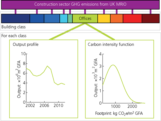
The UK BIEC model is implemented as a Matlab script that draws on two principal data sources. The first is a time series of aggregate construction sector embodied emissions from the UK MRIO model described by Giesekam et al. (2014). The second is a database of building-level LCA studies. The bulk of these studies are extracted from the Wrap Embodied Carbon Database (Wrap and UKGBC, 2014), with the remainder sourced from a variety of academic and industry publications. The database included 249 studies at the time the scenario analysis was completed. This figure has since increased and will continue to grow as carbon assessment becomes commonplace within the industry.
Each construction class is represented by a ‘carbon intensity function’ reflecting the range of embodied carbon dioxide equivalent (CO2e) per square metre of gross floor area (GFA) (kg CO2e/m2 GFA) observed within that class in the database. Past and future projected output of each class is represented as an output profile in terms of the annual floor area constructed (m2 GFA). From these two elements, an initial bottom-up estimate of the total carbon footprint of each class is calculated. The sum of these classes is compared with the sector total from the MRIO time series. The difference between these totals is redistributed to the different classes in proportion to their calculated bottom-up totals, and a calibration loop adjusts the corresponding carbon intensity functions until the new totals match (see Section 2.5 for further details). The model has been initially calibrated over the period 2001–2012.
The boundaries of the model are the embodied GHG emissions incurred in the full international supply chains supporting new-build buildings and infrastructure within the UK. The time period considered by the scenario analysis extends from 2001 to 2030. This period includes the completion of initial strategic targets set out in Construction 2025 and confirmed UK Carbon Budgets at the time of writing. Although the UK has longer-term reduction targets extending to 2050, the share of these targets attributable to the construction sector has yet to be determined and the uncertainty associated with longer-term predictions of demand for building stock is much greater.
This paper presents version 1.0 of the model. Future versions of the model are intended to incorporate the changes discussed in Section 4. The model structure and data sources are detailed further in the following paragraphs and the Supplementary Material.
2.1 Building classes
The ten classes adopted (housing, factories, warehouses, education, health, offices, entertainment, retail, miscellaneous and infrastructure) match roughly those used within the Office for National Statistics’ (ONS) Output in the Construction Industry data series (ONS, 2015) and are broadly concordant with classes in the Wrap Embodied Carbon Database (Wrap and UKGBC, 2014). As certain ONS classes, namely ‘oil, steel and coal’, ‘garages’ and ‘agriculture’, represent relatively small levels of diverse output without a significant number of corresponding LCA studies, these classes are incorporated into the broader ‘miscellaneous’ class. The ONS class ‘schools and universities’ was simplified to ‘education’.
2.2 Carbon intensity functions
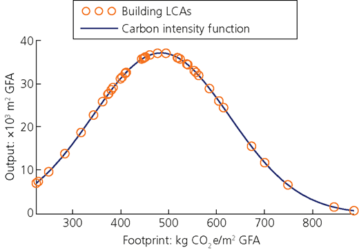
The carbon intensity functions draw on a database assembled from building-level LCAs categorised into the classes described previously. For each building class, the model extracts maximum and minimum observed values from the database, sorts the data by carbon intensity and plots and fits a probability density function. Figure 2 shows an example for housing. The quality of fit of each function depends on the number of LCA studies available for each class. For certain classes – that is, entertainment and factories – few LCA studies are available. The model user can specify a desired minimum sample size as an input. In instances where an insufficient sample is found in the database, the model defaults to carbon intensity functions that form a normal distribution around published embodied GHG emissions benchmarks for that building class (Rics, 2012).
This approach assumes implicitly that the LCAs in the database constitute a representative sample of structures within each class. This is unlikely to be the case. However, as further LCA studies are published, the sample size will grow. This will reduce the influence of individual studies on the computed carbon intensity functions and improve the model’s representation of reality.
In the case of classes composed of a diverse range of structures – that is, miscellaneous and infrastructure – it is not possible to gather information on typical builds. Therefore, for these two classes, a separate approach was adopted using average carbon intensity figures per UK pound of output from the Wrap Resource Efficiency Benchmarks (Wrap, 2014b).
2.3 Output profiles
Currently, no industry or public body gathers statistics on the cumulative floor area built each year. Consequently, it was necessary to assemble an estimate from a variety of data sources. Estimates for new-build housing floor area were computed by combining annual housing completions (DCLG, 2015a) with data representing the size of typical new-build homes (Riba, 2011). Non-domestic buildings pose a greater challenge as the government’s regular publication of commercial and industrial floor area statistics ceased in 1985 (Clark, 2013b). In the absence of reliable statistics, annual additions to stock for each class were estimated by combining the financial value of output published by the ONS with historical price data. Prices were obtained from numerous past editions of the industry standard Spon’s Architects’ and Builders’ Price Book (Aecom, 2015a), which provides estimated costs per square metre for a wide variety of building types. As the particular mix of new buildings within each class was unknown, it was necessary to assume that they were broadly in line with the proportions of the existing stock (Bruhns et al., 2000). Where the dominant form of building within each class is a particular building type, this was used as a representative average price for the class. Where new build within a class is composed of a diverse range of building types, an average price was calculated based on prices for multiple building types and their approximate share of the existing stock. By these means, approximate estimates of new-build floor area for each building class for 2001–2013 were established. See the Supplementary Material for further information.
2.4 Initial bottom-up emission estimate
When a model run begins, the carbon intensity function of each building class is scaled to the output profile for each year and the total embodied GHG emissions associated with producing that output is calculated. In the case of miscellaneous buildings and infrastructure, the bottom-up estimates are calculated directly by multiplying the financial value of the output by the carbon intensity per pound of output from the Wrap Resource Efficiency Benchmarks. These ten bottom-up estimates amount cumulatively to less than the top-down sector totals from the UK MRIO model. This is to be expected for two reasons. Firstly, the building-level LCAs in the database suffer from truncated system boundaries and the other typical shortcomings of process-based LCAs described by Lenzen (2000), Suh and Huppes (2005) and Majeau-Bettez et al. (2011). Secondly, the entries in the database are likely to represent better-than-average examples of each class, as practitioners that conduct carbon assessments and disseminate their results are more likely to seek to minimise embodied GHG emissions in their designs. For the model run reported in the following sections, the discrepancy between the bottom-up and top-down totals for each year is between 20 and 40%. Thus, a calibration process is required to correct for this discrepancy.
2.5 Model calibration
The calibration process is applied in two steps. Firstly, the difference between the top-down total from the MRIO and the initial bottom-up total is distributed between the building classes in proportion to their share of the initial bottom-up total. Thus, each class has a new target total. The model code then x-shifts the carbon intensity function by increments of 1 kg CO2e/m2 and produces a new bottom-up total. This process is looped until the bottom-up total is within 1% of the target total. The results of this calibration can be seen in Figure 3.
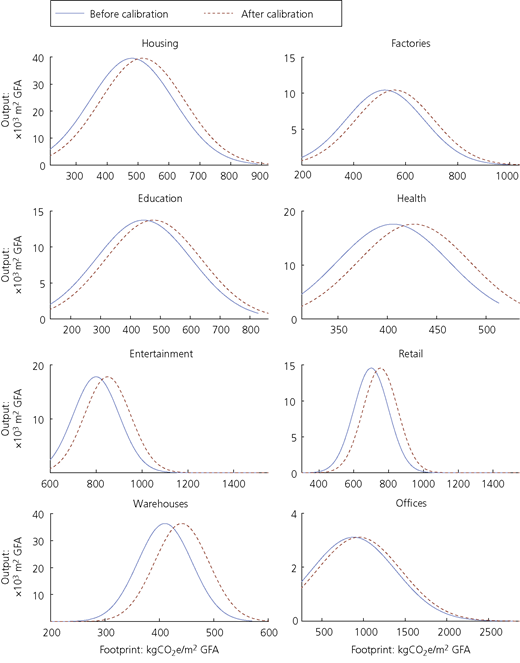
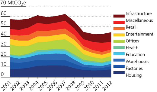
This process assumes inherently that the absolute difference between the reported embodied emissions figures and the true embodied emissions figures is the same on all projects. It is more likely that there are similar proportional differences. However, implementing a calibration loop that worked on this alternate assumption would increase complexity significantly. Given the inaccuracies in the underlying data and assumptions, a simple calibration process was deemed appropriate. By using this calibration process, a baseline time series of embodied emissions in the construction sector by building class was produced (see Figure 4).
3 Scenario analysis
Given the absolute nature of national Carbon Budgets, in essence, the greater the growth in construction activity, the less carbon-intensive that activity must be. Thus, growth in overall activity has the potential to impose more severe carbon reduction targets at the project level, necessitating the adoption of different reduction strategies. However, the level of aggregate demand and other key factors, such as the carbon intensity of the electricity supply, are beyond the control of the construction industry. Yet the industry will be expected to scale its ambitions in response to changes in these factors if it is to play an equal share in meeting long-term carbon reduction targets. The potential impact of these external factors is explored through a scenario analysis conducted in two phases. Firstly, a series of 27 plausible projections of future demand for buildings of each class were prepared, and the associated aggregate emissions were enumerated by extension of the UK BIEC output profiles. Required improvements in carbon intensity to meet sector targets were then considered through implementing changes in the carbon intensity functions of each class. The following sections consider these two phases in turn.
3.1 Future demand projections
The majority of detailed independent forecasts of construction output consider only the next 3–5 years (e.g. Aecom, 2015a; CPA, 2015; Experian, 2015). Long-term alternatives are restricted generally to very high-level forecasts, such as the Global Construction series (GCP and OE, 2013), and do not disaggregate projections beyond infrastructure, domestic and non-domestic properties. The long-term projections established for the routemap were largely based on historical trends and did not reflect current plans (Giesekam et al., 2014). Thus, as no robust, independent, disaggregated projections could be sourced, it was necessary to establish novel projections of new build.
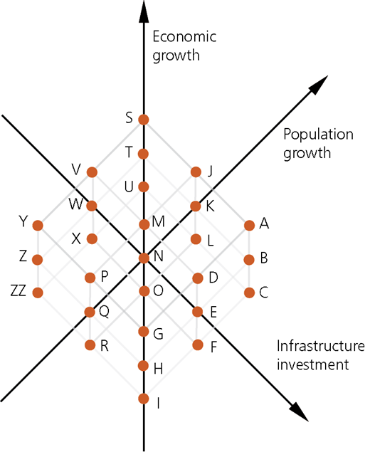
3.1.1 Estimating demand
Demand in the construction industry is dependent on a number of interconnected variables. In an attempt to simplify this complex system, projections were based on changes in three key variables: population, economic growth and infrastructure investment (see Figure 5). These projections drew on published projections of economic growth (HMT, 2015; OBR, 2012, 2015) population (ONS, 2011), households (DCLG, 2015b) and infrastructure investment (HMT, 2014), as summarised in Table 1 and described further in the Supplementary Material.
Variables used in demand projections
| Year | Low projection | Central projection | High projection | ||||||
|---|---|---|---|---|---|---|---|---|---|
| Economic growth: % | Population: million | Infrastructure investment(2012 = 100) | Economic growth: % | Population: million | Infrastructure investment (2012 = 100) | Economic growth: % | Population: million | Infrastructure investment (2012 = 100) | |
| 2013 | 1·7a | 63·405 | 108·60 | 1·7a | 63·758 | 108·60 | 1·7a | 63·999 | 108·60 |
| 2014 | 2·6a | 63·718 | 79·08 | 2·6a | 64·271 | 89·71 | 2·6a | 64·638 | 112·13 |
| 2015 | 2·1 | 64·017 | 85·71 | 2·5 | 64·776 | 93·44 | 3·0 | 65·285 | 116·80 |
| 2016 | 1·9 | 64·306 | 62·43 | 2·3 | 65·271 | 80·47 | 2·8 | 65·934 | 100·59 |
| 2017 | 1·9 | 64·582 | 54·18 | 2·3 | 65·755 | 79·44 | 2·8 | 66·578 | 99·30 |
| 2018 | 1·9 | 64·855 | 70·35 | 2·3 | 66·232 | 83·14 | 2·8 | 67·223 | 103·92 |
| 2019 | 1·9 | 65·124 | 62·32 | 2·3 | 66·705 | 78·00 | 2·8 | 67·869 | 97·50 |
| 2020 | 1·9 | 65·390 | 62·28 | 2·3 | 67·173 | 76·40 | 2·8 | 68·515 | 95·50 |
| 2021 | 1·9 | 65·652 | 62·31 | 2·4 | 67·636 | 81·81 | 2·9 | 69·159 | 106·24 |
| 2022 | 2·0 | 65·907 | 62·29 | 2·4 | 68·092 | 79·88 | 2·9 | 69·800 | 106·89 |
| 2023 | 2·0 | 66·155 | 63·91 | 2·4 | 68·539 | 79·78 | 2·9 | 70·436 | 105·04 |
| 2024 | 2·0 | 66·394 | 62·62 | 2·4 | 68·976 | 79·84 | 2·9 | 71·067 | 102·27 |
| 2025 | 2·0 | 66·622 | 62·68 | 2·4 | 69·404 | 79·28 | 2·9 | 71·692 | 100·51 |
| 2026 | 2·0 | 66·839 | 62·76 | 2·4 | 69·820 | 79·50 | 2·9 | 72·311 | 101·56 |
| 2027 | 2·0 | 67·044 | 62·85 | 2·4 | 70·226 | 80·02 | 2·9 | 72·925 | 102·52 |
| 2028 | 2·0 | 67·237 | 62·97 | 2·4 | 70·623 | 79·72 | 2·9 | 73·535 | 102·24 |
| 2029 | 2·0 | 67·416 | 62·78 | 2·4 | 71·011 | 79·69 | 2·9 | 74·141 | 102·74 |
| 2030 | 2·0 | 67·582 | 62·81 | 2·4 | 71·392 | 79·67 | 2·9 | 74·743 | 103·75 |
Confirmed
3.1.2 Projected grid decarbonisation
The carbon intensities of UK and international electricity grids are expected to reduce significantly over the analysis period, as existing plant is replaced with low carbon alternatives. A decomposition analysis of the UK MRIO reveals that, in 2011, 22% of the UK construction sector’s embodied GHG emissions footprint was attributable to electricity. By using these data and projected improvements in UK electricity emission factors from the Department of Energy and Climate Change (Decc, 2014; see Table 2), potential reductions in the construction sector’s embodied emissions attributable to improvements in grid intensity were projected. It should be noted that a portion of this footprint is associated with electricity grids outside of the UK. To avoid the complexity of determining grid projections for each foreign supplier, it has been assumed that all countries make equal proportional improvements to the UK. As it is impossible to determine from the available data the proportion of each building class’s footprint that is attributable to electricity, reductions have been applied uniformly across all classes.
Projected generation-based grid average electricity emissions factors from Decc (2014)
| Year | Emission factor: kg CO2e/kWh | Indexed to 2012 |
|---|---|---|
| 2012 | 0·494 | 100 |
| 2013 | 0·460 | 93·2 |
| 2014 | 0·461 | 93·4 |
| 2015 | 0·433 | 87·7 |
| 2016 | 0·339 | 68·6 |
| 2017 | 0·326 | 66·0 |
| 2018 | 0·308 | 62·3 |
| 2019 | 0·266 | 53·9 |
| 2020 | 0·238 | 48·2 |
| 2021 | 0·214 | 43·3 |
| 2022 | 0·198 | 40·0 |
| 2023 | 0·187 | 37·9 |
| 2024 | 0·167 | 33·8 |
| 2025 | 0·151 | 30·5 |
| 2026 | 0·126 | 25·5 |
| 2027 | 0·116 | 23·5 |
| 2028 | 0·103 | 20·8 |
| 2029 | 0·105 | 21·3 |
| 2030 | 0·102 | 20·7 |
3.1.3 Targets for comparison
To place the demand projections in context, they are compared with stated carbon reduction targets. Two sets of targets are considered: the recommended interim targets for embodied GHG emissions reduction from the routemap and the relative share of the UK Carbon Budgets attributable to the construction sector. To account for the differing baselines and accounting approaches, these targets were subject to the adjustments described in the Supplementary Material. This includes developing a set of equivalent consumption-based carbon budgets that consider UK emissions from a consumption rather than a territorial accounting approach. The headline 50% GHG emissions reduction target from Construction 2025 was also considered a potential point of comparison; however, as it is expressed as an aggregate target for all emissions from the built environment, it cannot be interpreted as a specific target for embodied GHG emissions.
3.2 Results
Results of the demand projections can be seen in Figure 6. The difference between the highest (A) and lowest (ZZ) projections represents additional annual embodied GHG emissions of 24·4 MtCO2e by 2030 and cumulative emissions of some 333 MtCO2e over the analysis period. Reduction in the GHG emissions (decarbonisation) of the grid is expected to reduce these impacts, as shown in Figure 7. Under the central projection (N), this would avoid annual emissions of 9·2 MtCO2e in 2030 and 105 MtCO2e over the analysis period.
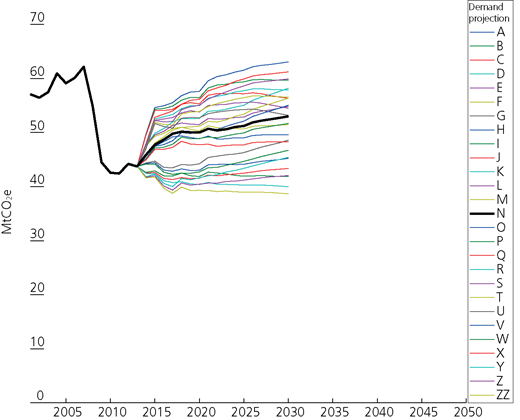
Projected embodied emissions of UK construction 2001–2030 assuming no improvements in carbon intensity of electricity supply
Projected embodied emissions of UK construction 2001–2030 assuming no improvements in carbon intensity of electricity supply
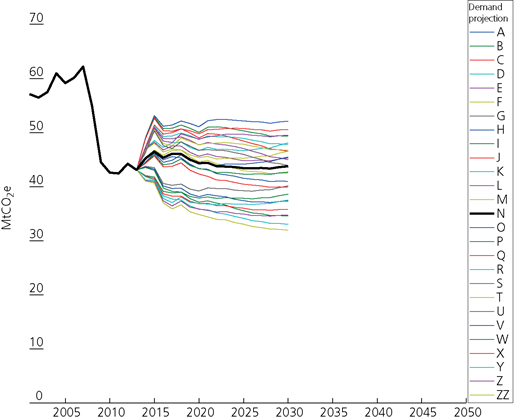
Projected embodied emissions of UK construction 2001–2030 including projected improvements in carbon intensity of electricity supply
Projected embodied emissions of UK construction 2001–2030 including projected improvements in carbon intensity of electricity supply
When compared with the consumption-based UK Carbon Budgets, the highest projection (A) anticipates that embodied GHG emissions in construction will grow from 5·1% of the first Carbon Budget to 9·0% of the fourth Carbon Budget. This includes anticipated grid decarbonisation, without which embodied GHG emissions could rise to 10·6%. Under the lowest projection (ZZ), embodied GHG emissions in construction represents 5·7% of the fourth Carbon Budget. Given the step change in national emission reductions anticipated under the fifth Carbon Budget, it is likely that embodied GHG emissions in construction will account for a sizeable proportion (>10%) of the available carbon space under all subsequent budgets.
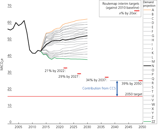
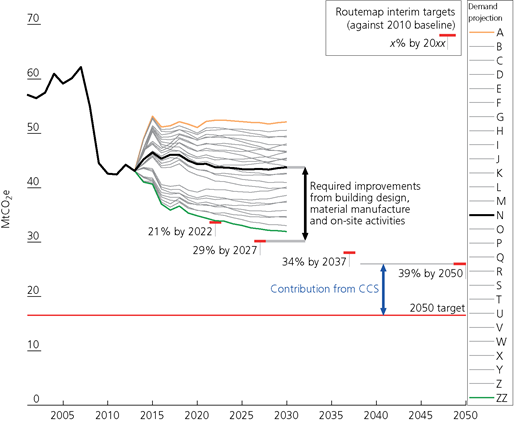
Figure 8 compares the demand projections with the interim targets proposed in the routemap. Figure 9 presents a similar comparison incorporating anticipated grid improvements. It is clear from such a comparison that considerable additional improvements in building design, material manufacture and on-site activities will be required if these targets are to be met. These improvements must be made in addition to Decc’s anticipated grid improvements and the full deployment of carbon dioxide capture and storage (CCS) technologies in steel and cement manufacture assumed in the routemap. If grid improvements do not occur at the expected rate, or CCS fails to become financially viable for material manufacturers, then the anticipated improvements required from designers would increase substantially. For example under the central projection N, if CCS is assumed to make no contribution by 2050 and the grid remains at the current carbon intensity, then meeting the 2027 routemap target would require more than double the level of improvements from building design, material manufacture and on-site activities. From a designer’s perspective, this may necessitate a fundamentally different set of building materials and structural forms.
Projected embodied emissions of UK construction 2001–2030 assuming no improvements in carbon intensity of electricity supply – relative to routemap interim targets
Projected embodied emissions of UK construction 2001–2030 assuming no improvements in carbon intensity of electricity supply – relative to routemap interim targets
Projected embodied emissions of UK construction 2001–2030 including projected improvements in carbon intensity of electricity supply – relative to routemap interim targets
Projected embodied emissions of UK construction 2001–2030 including projected improvements in carbon intensity of electricity supply – relative to routemap interim targets
To explore further the implication of assumptions about the grid, CCS uptake and future demand for stock, consider the following two extreme scenarios. Firstly, if it is assumed that demand proceeds along the lowest projection (ZZ), anticipated improvements in grid intensity are achieved and CCS uptake matches the routemap prediction, then at the project level designers need achieve only a 7% average improvement in carbon intensity compared with the current practice. This may well be achieved simply through the proliferation of the current best practice in design and would not require fundamental changes in materials or structural forms. However, if, by contrast, demand proceeds along the highest projection (A), the carbon intensity of the grid remains at current levels and there is no CCS, then designers may be faced with the prospect of making 67% reductions in carbon intensity across all projects by 2027 if the interim routemap targets are to be achieved. Such a high level of emissions reduction is likely to be impossible for certain building classes and would require widespread uptake of alternative materials and structural forms.
3.3 Discussion
These results highlight three sources of uncertainty that impact fundamentally on the changes in design and practice required by construction practitioners over the coming decades, namely the rate of grid electricity decarbonisation, the uptake of CCS and the overall demand for new building stock. All three of these factors are beyond the control of design teams, yet the response required from them to meet strategic emission reduction targets differs substantially depending on the assumed changes in these factors. Thus, while the targets are absolute, the scale of response required from the industry is deeply uncertain. In such an environment, it is difficult for practitioners and educators to anticipate the range of technologies, materials and practices that may need to be adopted and to develop appropriate skill sets. These multiple sources of uncertainty also make it difficult to propose policy solutions that are consistent with national carbon reduction targets.
While a range of options promoting demand reduction have been considered as part of long-term energy decarbonisation targets (e.g. Pye et al., 2014; Toke and Taylor, 2007), comparable actions to reduce demand for new buildings and infrastructure have yet to be considered. Indeed, the current government’s priority is to ‘keep Britain building’ (Osborne, 2015), apparently irrespective of the implication for carbon budgets. The deployment of low carbon technologies in energy provision, transport and other key economic sectors depends heavily on the widespread development of new infrastructure. However, neither the aggregate embodied emissions of these developments nor the corresponding volume of repair and maintenance that is sustainable in the long term has yet been determined. Even the otherwise comprehensive routemap considered only a solitary set of demand projections for future stock, implying that this is a variable that will not be deliberated. At the global level, the potential shortcomings of failing to consider the emissions embodied in infrastructure development have been highlighted by Müller et al. (2013), who demonstrated that the materials required for a globalisation of Western infrastructure stocks could consume 35–60% of the remaining global carbon budget until 2050 if the average temperature increase is to be limited to 2°C. Beyond 2050, the process-based emissions associated with manufacturing key materials for buildings and infrastructure development and maintenance may dominate the available carbon space. Put simply, in the future there may be zero-emission vehicles but there are unlikely to be zero-emission roads. Therefore, if the UK is to develop long-term infrastructure plans that are consistent with progressively tighter carbon budgets, then the appropriate aggregate level of demand for new stock must be considered. This debate is urgently required given the long lifetimes of buildings and infrastructure.
A further debate must focus on the role of materials producers within a low carbon economy. As UK production of bulk materials becomes less competitive and further significant investment in capacity appears unlikely, any increase in demand for materials will likely yield an increased dependence on imports with greater carbon intensity. Such a transition could drive a greater rise in embodied emissions than is projected in the scenarios. The changes in demand implied by a partial shift to alternative materials and an absolute reduction in the use of carbon-intensive materials may necessitate a rebalancing of the UK materials market, which is likely to have profound impacts on employment (Cooper et al., 2016). Few attempts have been made to quantify the structural changes or employment impacts of greater material efficiency on economies, and this area requires additional research urgently (Nathani, 2010). Ultimately, a coherent long-term vision for material production within a low carbon economy must be established such that the transition can be managed carefully.
4 Model limitations, future developments and applications
4.1 Model limitations
The model’s core database of building-level LCAs suffers from a number of shortcomings. Many of the LCAs are conducted to different standards, using different system boundaries and life cycle inventory (LCI) data sets, preventing them from being directly comparable. Thus, a component of the difference between entries is likely to be the decisions made by LCA practitioners rather than differences in design and material selection. As industry approaches are increasingly standardised, comparison between designs will become fairer. The sample of building-level LCAs used for the analysis is small relative to the number of structures produced annually in the UK and unlikely to be truly representative of sector output. The projects for which LCA studies are conducted may represent the better end of the spectrum of current practice, and the mix of project types may differ from those built within each class. For certain building classes, the dependence on published benchmarks is also undesirable. Furthermore, in calculating output profiles for some classes, the model depends on estimates of physical output computed from economic data. This carries a degree of uncertainty, although comparison between estimates of housing outputs using equivalent financial proxies and direct physical estimates suggests that the difference may be minor. The top-down estimate of sector emissions also suffers from the typical limitations of an IO approach described by Lenzen (2000) and Lindner (2013). The combined impact of these shortcomings is difficult to quantify and, consequently, it is advisable to view the results as being subject to significant uncertainty. However, the magnitude of these errors is unlikely to be large enough to undermine the principal trends.
4.2 Future model developments
In its current form, the model demonstrates a means to link sector-level targets with project-level targets by using the best available data. As more data are gathered, the model will be opened to a wider range of applications and results will command greater confidence.
Carbon intensity functions can be improved through the addition of more building LCAs. The increasing standardisation of approaches to measurement and reporting of embodied GHG emissions should also reduce the error in building comparisons. Disaggregation of the building classes into recognisable subclasses would allow designers to make more direct comparisons with model entries and projections. For instance, with collection of sufficient LCA entries, housing would be divided into detached, semi-detached, mid-terrace, end-terrace and so on. Further disaggregation of the infrastructure class in particular could build on projections of construction and future emissions submitted to regulators (e.g. Keil et al., 2013). Better statistics on physical outputs (i.e. completed floor areas) could also remove the dependence on financial proxies. The model will also undergo periodic updates with the latest emissions data.
4.3 Future model applications
Given a sufficient evidence base, the UK BIEC model could be used to assess simultaneously combined improvements in grid intensity, the introduction of regulatory limits, generic improvements in practice and the implications of practical design limits on required emission reductions. As additional data become available, the model could be used to monitor annual progress towards targets and provide indicative targets for design teams that are consistent with strategic sector and national emission reduction goals. This would allow practitioners to anticipate the sorts of materials and designs that may be required in the future and develop skills accordingly. A more heavily disaggregated model could also facilitate impact assessment of potential policy interventions.
5 Conclusions
The UK BIEC model provides an analytical framework that links sector-level embodied GHG emissions estimates with project-level calculations. A simple scenario analysis, based on the best available data, illustrates the scale of the challenge facing the construction sector if strategic GHG emissions reduction targets are to be achieved. Significant improvements in building design, material manufacture and on-site activities will be required and the range of materials and forms adopted in future will depend heavily on the rate of grid electricity decarbonisation, the uptake of CCS and the overall level of demand for new stock. While the analysis demonstrated the value of the initial link between sector and project targets, further development, including an expansion of the existing evidence base, will be required to increase the model accuracy and range of applications. The authors would welcome contributions to this from practitioners engaged in regular carbon assessment.
The scenario analysis also provided an indication of the potential role for demand reduction in meeting sector targets. However, as highlighted in the discussion, the aggregate embodied GHG emissions of building and infrastructure development has yet to be considered seriously by policymakers, and any form of demand reduction may run counter to the prevailing political narrative. The discussion also highlighted the lack of a coherent vision for materials production within a low carbon economy. Effective management of the transition to a low carbon construction sector will require development of a plan that considers both demand for new stock and the impacts on the supply chain. In the meantime, it is clear that practitioners and policymakers face multiple sources of uncertainty, making it difficult to distinguish the range of designs, materials and policy interventions that may be required under progressively tighter carbon budgets.
Acknowledgements
This work was financially supported by the Engineering and Physical Sciences Research Council (grant number EP/G036608/1). The contribution of the second author was supported by the Research Council UK Energy Programme through the Centre for Industrial Energy, Materials and Products (grant number EP/N022645/1). The authors would like to thank Dan Doran (Building Research Establishment) for assistance developing ideas for the model framework.
