
The article aims to establish whether the degree of aversion to inflation and the responsiveness to deviations from potential output have changed over time.
This paper assesses time variation in monetary policy rules by applying a time-varying parameter generalised methods of moments (TVP-GMM) framework.
Using monthly data until December 2022 for five inflation targeting countries (the UK, Canada, Australia, New Zealand, Sweden) and five countries with alternative monetary regimes (the US, Japan, Denmark, the Euro Area, Switzerland), we find that monetary policy has become more averse to inflation and more responsive to the output gap in both sets of countries over time. In particular, there has been a clear shift in inflation targeting countries towards a more hawkish stance on inflation since the adoption of this regime and a greater response to both inflation and the output gap in most countries after the global financial crisis, which indicates a stronger reliance on monetary rules to stabilise the economy in recent years. It also appears that inflation targeting countries pay greater attention to the exchange rate pass-through channel when setting interest rates. Finally, monetary surprises do not seem to be an important determinant of the evolution over time of the Taylor rule parameters, which suggests a high degree of monetary policy transparency in the countries under examination.
It provides new evidence on changes over time in monetary policy rules.
1. Introduction
In recent decades, monetary authorities in major central banks have managed to achieve low and stable inflation rates, which have been seen as a direct result of the adoption of monetary policy rules. Taylor rules appear to explain monetary policy well in inflation targeting countries (Taylor and Davradakis, 2006; Çağlayan and Astar, 2010; Neuenkirch and Tillmann, 2014), but even central banks which operate alternative monetary regimes are known to follow at times such a rule to stabilise inflation (Woodford, 2001; Orphanides, 2003; Sauer and Sturm, 2007; Sanchez-Robles and Maza, 2013; Nitschka and Markov, 2016). However, regardless of the type of monetary regime in place, policymakers and their objectives can change over time, and thus their monetary stance can also change to respond effectively to shocks.
Several studies have recognised this fact and investigated possible shifts in the parameters of monetary policy rules over time. Sub-period analyses in this context provide evidence for changing interest rate policies, but tend to focus primarily on the US, which experienced such changes during the Volcker-Greenspan era (Judd and Rudebusch, 1998; Clarida et al., 2000; Orphanides, 2004), while more complex regime-switching models have been used to capture shifts in the Taylor rule parameters in other developed as well as emerging economies (Zheng et al., 2012; Alba and Wang, 2017; Caporale et al., 2018). Other studies, which employ maximum likelihood (ML) and Kalman filtering methods, report that time-varying parameter (TVP) Taylor rules explain monetary policy better than constant parameter ones (Kim and Nelson, 2006; Trecroci and Vassalli, 2010; Yüksel et al., 2013). However, as Partouche (2007) points out, Kalman filter methods are restrictive since they impose constraints on the form of heteroscedasticity and the correlations between the disturbances and the regressors; he proposes using instead a version of the generalised methods of moments (GMM) which allows for time variation to capture changes in monetary policy rules and applies this framework to analyse the behaviour of the federal reserve.
The present paper contributes to this area of the literature by assessing how the stance of monetary authorities towards inflation and output stabilisation changes over time, as reflected in the Taylor rule parameters. We apply the procedure developed by Partouche (2007) to a greater range of countries with different monetary frameworks, and for an extended sample including recent crisis periods characterised by monetary policy shifts. More specifically, the analysis applies a TVP-GMM framework as in Partouche (2007) to estimate Taylor rules for five inflation targeting countries, i.e. the UK, Canada, Australia, New Zealand and Sweden. For comparison purposes, the exercise is also carried out for a set of countries which have instead adopted alternative monetary regimes but followed a Taylor rule at times, namely the US, Japan, Denmark, the Euro Area and Switzerland. Both standard and augmented forward-looking TVP Taylor rules are estimated and assessed against constant parameter rules. Importantly, the GMM method allows us to capture gradual changes in the monetary stance over long time periods which constant parameter rules or sub-sample analyses are unable to detect. Compared to other time-varying methods, the one used in this paper has several advantages; specifically, it uses smoothed estimates rather than filtered ones, does not impose any priors and deals with the endogeneity problem that arises from the presence of expected values in the regressors.
2. Literature review
Several monetary authorities around the world have been operating an inflation targeting regime since the 1990s, while central banks with alternative monetary frameworks have at times targeted the inflation rate according to a monetary policy rule. The well-known Taylor rule (Taylor, 1993, 1999b) describes monetary policy as an interest rate setting mechanism to respond to deviations of inflation and output from their targets. It has been found that monetary authorities who follow a Taylor rule experience greater macroeconomic stability (Fregert and Jonung, 2008; Çağlayan and Astar, 2010; Beaudry and Ruge-Murcia, 2017; Zhu et al., 2021). Further evidence suggests that monetary policy can best be described by a Taylor rule even in countries which did not adopt an inflation targeting framework, for instance the US (Woodford, 2001; Orphanides, 2003), the Euro Area (Sauer and Sturm, 2007; Sanchez-Robles and Maza, 2013), Switzerland (Nitschka and Markov, 2016) and the seven largest Latin American countries (Moura and De Carvalho, 2010).
It should be noted that, despite the increasingly widespread use of Taylor rules by monetary authorities, some issues arise when such a policy framework is adopted. For instance, some studies claim that the use of Taylor rules does not always generate the best economic outcomes. In particular, Crowley and Hudgins (2021) used a wavelet-based control model to compare the US Taylor rule to an optimal control policy rule. While the results indicate that the Taylor rule generates higher interest rates in a low inflation environment under both a hawkish and a dovish regime, they should be seen as mainly illustrative since the wavelet-based model is not fully calibrated. There are also other disadvantages to using Taylor rules. These include: the difficulty of estimating some unobservable variables such as the output gap; the limited availability of real time data on output and prices which would enable monetary authorities to respond more effectively to changes in those variables; the lack of parameters capturing directly its impact on the financial sector, for instance through its effects on the balance sheets of financial institutions.
A further issue concerns the use of monetary policy rules versus exercising monetary discretion. There is an ample debate in the literature, which is summarised by Taylor (2017) in his review paper discussing the main arguments of both sides. He concludes that a more systematic approach to monetary policy generates better economic outcomes since proposals for monetary policy rules tend to be based on the findings of empirical research and have improved over time. However, central banks are advised to improve their reporting on how these rules are being used.
It is important to point out that various specifications of the Taylor rule have been considered in the existing literature, and also that various methods have been used for their estimation. The augmented Taylor rule, which includes the real exchange rate in addition to the inflation and output gaps, seems to explain monetary policy well in open economies (Batini et al., 2003; Adolfson, 2007; Aizenman et al., 2011), and forward-looking rules in particular have found much support in the literature (Batini and Haldane, 1998; Fendel et al., 2011; Nikolsko-Rzhevskyy, 2011). The methods used include ordinary least squares (OLS), ML and system methods (Cochrane, 2011). The seminal paper by Clarida et al. (1998) was the first to apply the GMM framework to forward-looking Taylor rules; its findings suggest that monetary policy can be explained accurately using this method in the case of the G3 (Germany, Japan and the US) and to some extent in that of the E3 (the UK, France and Italy). Subsequent empirical studies found that GMM is the most suitable methodology to deal with endogeneity when estimating monetary policy rules (Florens et al., 2001; Yau, 2010; Rühl, 2015).
It must be stressed that monetary policy objectives can change over time. Therefore a key issue in this context is the adoption of a modelling framework which allows for time variation in the Taylor rule parameters. Judd and Rudebusch (1998), for instance, performed a sub-sample analysis of the Fed’s policy rule using OLS and found substantial differences in the parameters between the sub-periods considered. Clarida et al. (2000) assessed forward-looking Taylor rules in a GMM framework and reported significant monetary policy regime shifts for the Fed during the Volcker-Greenspan era. Similar results were obtained by Orphanides (2004) when including real-time information in the model. McCulloch (2007) used an adaptive least squares approach and confirmed previous findings that the parameters in the US Taylor rule are not constant. Conrad and Eife (2012) performed rolling window regressions to obtain TVP estimates of the Taylor rule reaction function for the Fed, their findings also explaining changes in the US inflation-gap persistence. Papadamou et al. (2018) applied the GMM method to conduct sub-sample analysis for a period including the global financial crisis and found evidence of substantial asymmetries in the ECB’s reaction function. Orphanides and Williams (2005) adopted a TVP vector autoregressive (VAR) framework and found that their model provided a good description of US monetary policy. Similar results were obtained by Sims and Zha (2006), who employed a structural VAR model with TVP. Several studies have modelled time variation by using regime-switching models. Caporale et al. (2018), for instance, estimated augmented Taylor rules for selected emerging economies by using a Threshold GMM, which seems to capture well the behaviour of central banks in those countries. Markov-switching and Smooth Transition applications also provide ample evidence for parameter shifts in the monetary policy rule for various developed and emerging economies (Perruchoud, 2009; Alcidi et al., 2011; Zheng et al., 2012; Alba and Wang, 2017).
More recent studies employ a Kalman filtering approach to model policy shifts and structural changes in the Taylor rule. Trecroci and Vassalli (2010) found that a TVP specification using the Kalman filter outperforms the constant parameter one by capturing changes in the monetary policy rule for the US, the UK, Germany, France and Italy. Yüksel et al. (2013) applied the extended Kalman filter to estimate TVPs in the monetary policy rule in the case of Turkey, and found that this specification outperforms the standard one for the central bank reaction function. Boivin (2006) used the Kalman filter to estimate a likelihood function for the US and found evidence of gradual changes in the Taylor rule parameters. Using a two-step ML method, Kim and Nelson (2006) showed that US monetary policy can be classified according to three distinct periods with different Taylor rule parameters rather than the two identified previously.
The effectiveness of monetary policy rules also depends on how they are perceived by the public. Bauer et al. (2022) analysed this issue in the case of the US and noticed significant changes over time. Specifically, the output coefficient decreases (increases) towards the end (beginning) of a tightening cycle and monetary easings tend to be implemented quickly, while tightenings occur more gradually. Bianchi et al. (2022) documented large shifts in the parameters of the US monetary policy rule over the past few decades and concluded that infrequent changes in the monetary stance can lead to persistent shifts in the real interest rate and asset valuations. Bauer and Swanson (2023) estimated a time-varying monetary policy rule for the Fed using weighted recursive least squares and found that the Fed’s response to both the inflation and output gap has increased over the past 3 decades. Using a ML estimation method, Gürkaynak et al. (2023) provided evidence that weak monetary rules not satisfying the Taylor principle lead to out-of-control inflation.
Although most of the abovementioned studies suggest that the Kalman filter captures gradual variations in the Taylor rule better than constant parameter models, this approach suffers from a major drawback, since it imposes constraints on the form of heteroscedasticity of the error term. To address this issue, Partouche (2007) developed a GMM framework with TVPs to assess parameter shifts in the monetary policy rule. This model has the advantage that it is robust to heteroscedasticity, unlike Kalman filtering approaches, and is applied in the present study to carry out the empirical analysis.
3. Empirical framework
3.1 The Taylor rule
Taylor (1993, 1998) proposes the following monetary rule to capture the behaviour of a central bank:
where is the policy rate, is the inflation rate and the inflation target, is the output gap, i.e. the deviation of real gross domestic product (GDP) from target, and is the equilibrium real interest rate. The size of the parameters and indicates the central bank’s degree of inflation aversion (higher ) compared to unemployment aversion (higher ), and were originally set equal to and respectively in Taylor (1998).
The empirical Taylor rule estimated in this paper is a forward-looking one of the following form:
where is the interest rate set by the central bank, and is the equilibrium real interest rate, which is unobserved and is measured by the constant in the regression as in most studies (e.g. Razzak, 2003; Adanur Aklan and Nargelecekenler, 2008; Belke and Klose, 2009; Judd and Rudebusch, 2020). and are the -period ahead forecasts of inflation and the output gap respectively, and is an error term. Instead of contemporaneous or lagged values of the variables, we include proxies for forecasts based on the 3-month lead average for the inflation rate and the output gap. Since backward-looking specifications of the Taylor rule have been rejected in favour of forward-looking ones, the above should capture monetary policy more accurately (Clarida et al., 1998).
The Taylor rule given by equation (2) is suitable for closed economies; however, in open economies, monetary policy can be influenced by the behaviour of the real exchange rate, which has been considered in several studies (Svensson, 2000; Caporale et al., 2018; Tiryaki et al., 2018). Therefore, we also estimate the following augmented Taylor rule:
where is the forward-looking real effective exchange rate. We use the generalised methods of moments (GMM) framework to estimate the Taylor rules in equations and .
3.2 The constant parameter GMM
The GMM is a semi-parametric framework which is a suitable alternative to OLS approaches in cases where the error term is correlated with the regressors. This is likely to happen in forward-looking models which include (expected) future rather than contemporaneous values of the regressors; these are then correlated with the expectational errors usually contained in the error term (Taylor and Davradakis, 2006).
The estimation of a GMM model with constant parameters follows a two-step procedure as outlined in Clarida et al. (2000). Let denote a vector of instruments which satisfy the orthogonality condition . The GMM framework with an optimal weighting matrix accounts for any possible serial correlation in the error term . The weighting matrix depends on the population moments and the model parameters :
where stands for the endogenous variable in the model (in our case the policy rate), and for the explanatory variables. The moment conditions in the static parameter case are:
For cases where the number of instruments exceeds the number of parameters, overidentifying restrictions need to be imposed. We use the Sargan Test (Sargan, 1958) for the validity of the instruments in the overidentified case. Since this method requires all variables to be stationary, we carry out unit root tests for all of them, specifically the Dickey-Fuller generalised least squares (DF-GLS) test, the Zivot and Andrews (2002) test allowing for a break in the intercept and/or the trend, and the Lee and Strazicich (2003) Lagrange multiplier test allowing for a structural break under both the null and the alternative hypothesis.
To detect the possible presence of time-variation, one can estimate in the first instance a constant coefficient GMM model for some suitably identified sub-samples. This is often done in the literature (see, e.g. Orphanides, 2004; Papadamou et al., 2018) to distinguish between periods characterised by different policy regimes. Following this approach, we split the sample into sub-periods, first doing visual inspection of the inflation and policy rate series to determine the break points and next applying a more rigorous method, namely the structural break test developed by Andrews (1993), to detect the unknown break points.
3.3 A GMM model with time-varying parameters
While sub-period analysis can provide some evidence on time-variation in the Taylor rule parameters, the choice of the break dates could be arbitrary and the sub-periods too short for reliable statistical inference. Furthermore, this approach can only capture discrete parameter shifts. By contrast, the method suggested by Partouche (2007) allows for gradually evolving parameters within a GMM framework. Specifically, the minimisation problem in equation can be written as follows using the Lagrange multiplier:
with the underlying statistical model:
where is the Lagrange multiplier and is the covariance matrix of the innovation of the time-varying coefficient vector . Note that is assumed to follow a random walk. The corresponding moment conditions in the time-varying case are:
where the subscript denotes the time-varying element.
The problem in equation can be solved using non-parametric smoothing splines rather than the semi-parametric constant parameter GMM (Craven and Wahba, 1978). This method allows to carry out the estimation independently of a specific statistical model. The values of and are then chosen so as to obtain the estimates with the lowest mean squared error (MSE).
Modelling time variation in the parameters of the GMM directly is a more flexible method than sub-period analysis, and it does not face the issue of the small numbers of observations within sub-periods. Unlike the Kalman filtering approach suggested by Kim and Nelson (2006), which requires assuming a specific form of heteroscedasticity, the TVP-GMM framework is robust to the type of heteroscedasticity in the errors. To deal with possible autocorrelation, Stock and Watson (1998) suggest using an autoregressive filter, whilst the endogeneity problem can be addressed by using the median unbiased estimate calculation developed by Stock and Watson (1998).
Partouche (2007) recommends checking robustness with respect to the covariance matrix . In particular, in the TVP-GMM model, the variance of the innovations is constrained to be diagonal. Following Partouche (2007), we redo the estimation after removing this restriction. Finally, as an additional robustness test, we also estimate TVPs in a backward-looking version of the standard and augmented Taylor rules by entering the first lags of the regressors.
4. Data and empirical results
4.1 Data description
We estimate the Taylor rule for countries which adopted an inflation targeting regime in the early 1990s, namely the UK, Canada, Australia, New Zealand and Sweden, as well as for a set of countries with alternative monetary regimes which, however, have at times followed a policy rule, more precisely, the US, Japan, Denmark, the Euro Area and Switzerland. We use monthly data from January 1985 up until December 2022 for all countries except the Euro Area, for which data are only available from January 1999 [1]. The classification of countries into inflation targeters and those with alternative monetary regimes is made on the basis of which ones adopted the inflation targeting regime during the 1990s and is consistent with those found in the existing literature (Mishkin and Schmidt-Hebbel, 2001). While there are some minor disagreements concerning the defining characteristics of the inflation targeting framework (Sterne, 2000), in general countries are classified on the basis of the clarity and credibility of their commitment to the target over the entire sample range under consideration; according to this criterion the first set of countries in our case are full-fledged inflation targeters, while the others operate an implicit price stability anchor (Carare and Stone, 2006). Full-fledged inflation targeters make a full commitment to the inflation target and tend to have a higher level of credibility due to an institutionalised transparent monetary policy framework. Countries with an implicit price stability anchor are able to maintain low and stable inflation without displaying full transparency in relation to an inflation target. This allows these countries to pursue dual objectives of output and price stabilisation.
The consumer price inflation (CPI) series have been obtained from the Bank for International Settlements (BIS) consumer prices dataset for all countries and used to construct the inflation gap [2]. The interest rate series is the central bank policy rate which has been taken from the BIS Central Bank Policy Rates dataset. The output series is the organisation for economic co-operation and development (OECD) normalised GDP series obtained from the federal reserve bank of St Louis economic database (FRED). The Hodrick-Prescott filter is used to estimate the output gap [3]. The real effective exchange rate series have been retrieved from the BIS effective exchange rate narrow indices dataset. We also obtain from Bloomberg central bank announcements together with forecasts of interest rate decisions; this allows us to establish whether an announcement included an unexpected component , which is the difference between what the central bank announces () and what the market expected , i.e. . A value of which is different from zero indicates that the central bank is implementing stronger monetary policy measures than anticipated by the market. Details regarding the announcement dates for all countries are included in Online Appendix A. This information helps to interpret the evolution of the Taylor rule parameters over time. As instruments in both the constant and the TVP-GMM models we use a constant and the first, third, sixth and twelfth lag of the interest rate, the inflation rate and the output gap to estimate the standard Taylor rule as in equation , and for the augmented Taylor rule as in equation we include the first, third, sixth and twelfth lag of the real effective exchange rate as additional instruments.
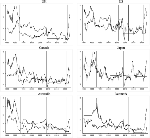
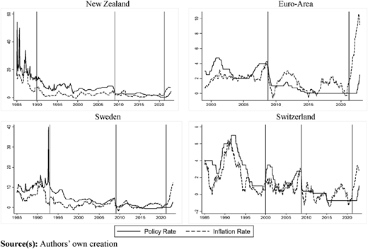
Figure 1 plots the inflation and interest rate series for each country over time. Vertical lines correspond to the main shifts in monetary policy. For inflation targeting countries, this includes the point when the inflation targeting regime was officially adopted, but also turning points when the attitude towards inflation changed – for instance, immediately after the global financial crisis, when several countries resorted to unconventional monetary policies, such as quantitative easing and forward guidance. For countries with alternative monetary policy regimes the vertical lines indicate points in time when the respective central banks began to use actively a monetary policy rule to target the inflation rate. Monetary policy appears to have been contractionary in almost all countries up until the global financial crisis, when it became more accommodating. Noticeable changes in inflation and policy rate behaviour occurred also as a result of the recent Covid-19 pandemic. However, a split of the full sample into subsamples around these dates would result in insufficient data points to allow for meaningful statistical inference.
Before starting the empirical estimation we test for stationarity of the individual time series since this is a requirement of the GMM model. Table 1 reports the results of the three unit roots tests we carry out. The DF-GLS and the Lee and Strazicich tests indicate that all series are stationary except the real effective exchange rate ones, which are integrated of order I(1) and therefore are entered into the model in first differences; however, the Zivot-Andrews test implies that in some cases the policy and inflation rates are also integrated of order I(1).
DF-GLS, Zivot-Andrews (ZA) and Lee and Strazicich (LS) unit root test results for the individual series
| DF-GLS | ZA | LS | DF-GLS | ZA | LS | |
|---|---|---|---|---|---|---|
| United Kingdom | −3.237** | −2.309 | −5.901*** | −4.898*** | −9.377*** | −9.765*** |
| Canada | −3.784*** | −3.750 | −5.720*** | −4.680*** | −9.153*** | −9.381*** |
| Australia | −5.122*** | −2.897 | −6.236*** | −7.502*** | −7.449*** | −12.754*** |
| New Zealand | −3.552*** | −2.878 | −5.609*** | −5.025*** | −11.443*** | −12.821*** |
| Sweden | −3.361** | −3.815 | −5.442*** | −11.951*** | −12.285*** | −12.383*** |
| United States | −3.084** | −2.644 | −4.613** | −11.670*** | −9.807*** | −5.330*** |
| Japan | −3.889*** | −4.797** | −4.238** | −11.415*** | −17.709*** | −25.812*** |
| Denmark | −3.303** | −2.892 | −4.291** | −4.072*** | −17.387*** | −17.154*** |
| Euro-Area | −3.168** | −1.112 | −5.170*** | −10.758*** | −17.847*** | −17.662*** |
| Switzerland | −3.291** | −3.040 | −3.002 | −6.561*** | −17.647*** | −11.876*** |
| United Kingdom | −5.112*** | −6.114*** | −5.528*** | −6.681*** | −11.990*** | −6.509*** |
| Canada | −5.246*** | −5.331*** | −5.233*** | −10.136*** | −10.298*** | −10.083*** |
| Australia | −5.248*** | −5.214*** | −5.328*** | −4.590*** | −10.628*** | −10.636*** |
| New Zealand | −3.323** | −6.430*** | −4.537*** | −6.580*** | −9.602*** | −8.915*** |
| Sweden | −5.970*** | −4.453** | −5.558*** | −6.235*** | −7.350*** | −6.350*** |
| United States | −5.431*** | −5.707*** | −5.317*** | −7.660*** | −9.544*** | −9.598*** |
| Japan | −5.560*** | −5.240*** | −5.606*** | −6.038*** | −7.859*** | −7.312*** |
| Denmark | −4.154*** | −6.070*** | −4.742*** | −7.203*** | −8.891*** | −7.348*** |
| Euro-Area | −3.802*** | −4.425** | −4.465** | −11.715*** | −12.067*** | −12.458*** |
| Switzerland | −5.185*** | −4.845** | −4.447** | −6.443*** | −10.743*** | −6.799*** |
| United Kingdom | −3.160** | −4.166 | −4.832*** | −8.709*** | −12.397*** | −9.160*** |
| Canada | −5.141*** | −4.501** | −6.807*** | −8.140*** | −10.373*** | −8.676*** |
| Australia | −3.327** | −3.889 | −4.004** | −5.589*** | −21.285*** | −21.347*** |
| New Zealand | −3.792*** | −3.519 | −3.664 | −6.394*** | −21.294*** | −6.543*** |
| Sweden | −3.504*** | −4.425** | −3.681 | −5.597*** | −11.695*** | −11.699*** |
| United States | −4.084*** | −5.801*** | −5.406*** | −8.079*** | −12.165*** | −7.890*** |
| Japan | −4.951*** | −6.672*** | −5.085*** | −14.245*** | −13.612*** | −13.428*** |
| Denmark | −3.220** | −2.831 | −4.125** | −5.466*** | −12.765*** | −13.028*** |
| Euro-Area | −3.005** | −3.265 | −4.830*** | −4.675*** | −6.995*** | −16.790*** |
| Switzerland | −3.495*** | −5.127*** | −4.704*** | −12.045*** | −12.616*** | −12.760*** |
| United Kingdom | −2.562 | −3.471 | −3.731 | −5.537*** | −11.066*** | −11.305*** |
| Canada | −1.750 | −2.109 | −2.431 | −3.549*** | −9.366*** | −9.779*** |
| Australia | −1.561 | −2.929 | −3.140 | −5.646*** | −14.709*** | −13.304*** |
| New Zealand | −2.342 | −3.423 | −3.164 | −4.776*** | −11.665*** | −6.628*** |
| Sweden | −2.739 | −3.505 | −4.002** | −3.601*** | −13.746*** | −14.352*** |
| United States | −0.605 | −3.968 | −2.650 | −5.883*** | −14.439*** | −13.586*** |
| Japan | −1.569 | −3.716 | −3.707 | −3.841*** | −10.356*** | −10.539*** |
| Denmark | −1.681 | −4.322 | −4.837*** | −3.257** | −14.710*** | −14.780*** |
| Euro-Area | −2.331 | −4.248 | −2.817 | −3.135** | −12.069*** | −12.225*** |
| Switzerland | −2.708 | −3.264 | −3.425 | −3.881*** | −11.722*** | −11.796*** |
Note(s): * significant at 10% level, ** significant at 5% level, *** significant at 1% level
DF-GLS test hypothesis: , , The tests include both a constant and linear trend as both are statistically significant. Zivot-Andrews test hypothesis: , , Tests for a break in both intercept and trend. Lee and Strazicich test hypothesis: , , Tests for a break in both intercept and trend
Source(s): Authors’ own creation
This is not an uncommon finding; nevertheless, many authors, such as Clarida et al. (1998, 2000), treat the policy rate and in some cases also the inflation rate as stationary, which they view as a reasonable assumption to estimate the Taylor rules without too much information loss from differencing. For this reason, and given the fact that the majority of the unit root tests we employ suggest that both these variables are stationary, we also treat them as such.
4.2 Results for the constant parameter taylor rule
For a start we estimate the standard and augmented Taylor rules using the constant parameter GMM for the entire sample and report the results in Table 2 for all countries. On first inspection one can note that the coefficients on the inflation and output gap are not particularly close to the values of 1.5 and 0.5 suggested by Taylor (1998). The inflation gap parameters range between 1.09 and 2.23 and the output gap ones between 0.32 and 0.82 for the countries in our sample. The real effective exchange rate included in the augmented Taylor rule seems to play an important role mainly in the case of Australia and Sweden, whilst it is less relevant in the other cases.
Constant parameter GMM results for the full sample
| Sargan test | ||||||
|---|---|---|---|---|---|---|
| United Kingdom | Standard | 1.7817*** | 1.3449*** | 0.3187** | – | 0.2586 |
| (0.1458) | (0.2647) | (0.1471) | – | |||
| Augmented | 0.9997*** | 1.1259*** | 0.3089** | 0.0160*** | 0.4289 | |
| (0.0176) | (0.2858) | (0.1290) | (0.0011) | |||
| Canada | Standard | 1.7536*** | 1.6404*** | 0.8117*** | – | 0.3287 |
| (0.1705) | (0.2786) | (0.1955) | – | |||
| Augmented | 5.1436*** | 1.6239*** | 0.3265** | −0.0310 | 0.7383 | |
| (1.1107) | (0.2271) | (0.1621) | (0.0100) | |||
| Australia | Standard | 1.1849*** | 0.4671*** | 0.5258*** | – | 0.2053 |
| (0.2116) | (0.0916) | (0.1879) | – | |||
| Augmented | 1.6268*** | 0.5487*** | 0.7800*** | 0.5349** | 0.7975 | |
| (0.1150) | (0.1151) | (0.2571) | (0.1901) | |||
| New Zealand | Standard | 3.7458*** | 0.7886*** | 0.8215*** | – | 0.1376 |
| (0.0797) | (0.0540) | (0.2890) | – | |||
| Augmented | 1.4981*** | 0.6428*** | 0.4049*** | −0.0411*** | 0.4302 | |
| (0.0799) | (0.1156) | (0.1406) | (0.0087) | |||
| Sweden | Standard | 0.7525*** | 1.4415*** | 0.5082** | – | 0.1915 |
| (0.1766) | (0.3284) | (0.2123) | – | |||
| Augmented | −0.8318*** | 1.1942*** | 0.2945** | 0.1441*** | 0.6648 | |
| (0.0231) | (0.3811) | (0.1476) | (0.0159) | |||
| United States | Standard | 1.3516*** | 2.2289*** | 0.5012 | – | 0.6254 |
| (0.1988) | (0.4419) | (0.3146) | – | |||
| Augmented | 1.2051*** | 1.6267*** | 0.7833** | −0.2621 | 0.3776 | |
| (0.1821) | (0.3626) | (0.3412) | (0.6842) | |||
| Japan | Standard | 0.4518** | 1.6097*** | 1.1090*** | – | 0.1039 |
| (0.2183) | (0.1336) | (0.1685) | – | |||
| Augmented | 0.4911** | 1.5800*** | 1.0321*** | 0.0914 | 0.2314 | |
| (0.2173) | (0.1547) | (0.1914) | (0.1656) | |||
| Denmark | Standard | 0.7385*** | 0.9078*** | 0.0561 | – | 0.1074 |
| (0.0858) | (0.0787) | (0.1368) | – | |||
| Augmented | 0.7121*** | 0.9028*** | 0.0675 | 0.5901 | 0.2607 | |
| (0.0876) | (0.0979) | (0.1366) | (0.4862) | |||
| Euro-Area | Standard | 0.8326** | 1.2938*** | 0.2584 | – | 0.2239 |
| (0.3573) | (0.1946) | (0.1995) | – | |||
| Augmented | −2.0375 | 1.0908*** | 0.5412*** | 0.0142 | 0.3793 | |
| (2.4212) | (0.2351) | (0.1664) | (0.0216) | |||
| Switzerland | Standard | 2.2613*** | 1.4127*** | 0.4490** | – | 0.2548 |
| (0.3257) | (0.0772) | (0.2271) | – | |||
| Augmented | 5.8376*** | 1.2209*** | 0.3293** | 0.0408** | 0.3418 | |
| (1.6809) | (0.0965) | (0.1376) | (0.0200) |
Note(s): * significant at 10% level, ** significant at 5% level, *** significant at 1% level
Standard errors in parentheses. The regression specification for the standard Taylor rule is that in equation (2), while the specification for the extended Taylor rule is that in equation (3). Overidentification restrictions are tested using the Sargan J-Test with probabilities reported
Source(s): Authors’ own creation
No significant differences emerge in the Taylor rule parameters between inflation targeting countries and those which adopted an alternative monetary regime instead. For the US, the coefficients are higher than those reported by some previous studies such as Österholm (2005) and Castro (2011), but very close to those estimated for the post-1982 period by Silva et al. (2021). They also seem to be higher for the case of Australia and Sweden compared, for instance, to those in Österholm (2005), while for the UK, New Zealand and the Euro Area they are lower than those reported in the previous literature (Castro, 2011; Kendall and Ng, 2013), although for sample periods rather different from that of the present study.
Next we perform sub-period analysis for both types of Taylor rules. At first, the sample is split into two sub-samples for each country according to the break dates identified from visual inspection of the series and corresponding to the main policy shift in each country (see Online Appendix B for details); note that creating more sub-samples would make the inference unreliable owing to the small number of observations in each case. Table 3 reports these results. The parameters seem to have changed significantly in most countries. More specifically, the inflation gap coefficients are lower in both sub-periods than the full-sample ones and now range between 0.38 and 1.32, whilst the output gap coefficients are mainly insignificant and range between 0.10 and 0.89.
Constant parameter GMM results with sub-period comparison with visual break point determination
| Sub-period | Sargan test | ||||||
|---|---|---|---|---|---|---|---|
| United Kingdom | Standard | 1985:1–2009:2 | 2.0280*** | 0.4263*** | 0.1127*** | – | 0.2844 |
| 2009:3–2022:12 | 0.6623*** | 0.0862 | 0.0650 | – | 0.7460 | ||
| Augmented | 1985:1–2009:2 | 4.6656*** | 0.4702*** | 0.0717 | 0.0229*** | 0.5581 | |
| 2009:3–2022:12 | 2.8348* | 0.2325 | 0.1497*** | 0.0190 | 0.7193 | ||
| Canada | Standard | 1985:1–2009:2 | 1.8616*** | 0.6037*** | 0.0509 | – | 0.1620 |
| 2009:3–2022:12 | 0.6192*** | 0.5930*** | 0.0836 | – | 0.3777 | ||
| Augmented | 1985:1–2009:2 | 0.5029 | 0.5208*** | 0.0321 | 0.0118*** | 0.4692 | |
| 2009:3–2022:12 | 4.1342*** | 0.5520*** | 0.0286 | 0.0323*** | 0.4857 | ||
| Australia | Standard | 1985:1–2009:2 | 2.0076*** | 0.3780*** | 0.2499*** | – | 0.2052 |
| 2009:3–2022:12 | 0.7704** | 1.1906*** | 0.0230 | – | 0.2832 | ||
| Augmented | 1985:1–2009:2 | 1.8081*** | 0.3838*** | 0.2431*** | 0.0668 | 0.2618 | |
| 2009:3–2022:12 | 0.9820** | 1.2566*** | 0.3153 | 0.7365** | 0.3400 | ||
| New Zealand | Standard | 1985:1–2009:2 | 3.1846*** | 1.0709*** | 0.8930*** | – | 0.0965 |
| 2009:3–2022:12 | 2.8008*** | 0.1379 | 0.7645 | – | 0.8410 | ||
| Augmented | 1985:1–2009:2 | 1.2420 | 0.4684*** | 0.0240 | 0.0088 | 0.8885 | |
| 2009:3–2022:12 | 1.7630 | 0.0590 | 0.4561 | 0.0089 | 0.5553 | ||
| Sweden | Standard | 1985:1–2009:2 | 1.5008*** | 0.5784*** | 0.0542 | – | 0.1417 |
| 2009:3–2022:12 | 1.0279*** | 0.2022 | 0.1024 | – | 0.2327 | ||
| Augmented | 1985:1–2009:2 | 1.4921*** | 0.5959*** | 0.0948 | 0.4427** | 0.7223 | |
| 2009:3–2022:12 | 0.4838 | 0.2812 | 0.0279 | 0.2064 | 0.6930 | ||
| United States | Standard | 1985:1–2011:12 | 1.4947*** | 1.1820*** | 0.1888 | – | 0.4244 |
| 2012:1–2022:12 | 1.5057*** | 0.5294*** | 0.1143 | – | 0.5105 | ||
| Augmented | 1985:1–2011:12 | 1.5077*** | 1.0574*** | 0.2121 | 0.0537 | 0.6010 | |
| 2012:1–2022:12 | 1.7893*** | 0.6971** | 1.5594 | 0.5802 | 0.6319 | ||
| Japan | Standard | 1985:1–2012:12 | 0.9308*** | 1.3223*** | 0.4237*** | – | 0.0997 |
| 2013:1–2022:12 | −2.2996*** | 0.0026 | 0.0075 | – | 0.2347 | ||
| Augmented | 1985:1–2012:12 | 0.8392*** | 1.2815*** | 0.3707*** | 0.0656 | 0.2188 | |
| 2013:1–2022:12 | −2.5901*** | 0.1751** | 0.1631 | 0.0563 | 0.2583 | ||
| Denmark | Standard | 1985:1–2011:10 | 1.2101*** | 0.3912*** | 0.1010** | – | 0.2169 |
| 2011:11–2022:12 | −0.4845 | 0.0701 | 0.0769 | – | 0.5639 | ||
| Augmented | 1985:1–2011:10 | 1.2097*** | 0.3874*** | 0.0779 | 0.0827 | 0.4267 | |
| 2011:11–2022:12 | −0.5010** | 0.0801 | 0.0744 | 0.1887 | 0.8195 | ||
| Euro-Area | Standard | 1985:1–2008:9 | 2.5416*** | 0.0962 | 0.7390*** | – | 0.1555 |
| 2008:10–2022:12 | −0.2033 | 0.4564** | 0.1392 | – | 0.3102 | ||
| Augmented | 1985:1–2008:9 | 9.2304*** | 0.4160 | 0.6263*** | 0.0526*** | 0.3172 | |
| 2008:10–2022:12 | −7.6741*** | 0.2106 | 0.0471 | 0.0764*** | 0.0590 | ||
| Switzerland | Standard | 1985:1–2008:9 | 2.8604*** | 1.2634*** | 0.0092 | – | 0.1672 |
| 2008:10–2022:12 | −0.6278 | 0.9355** | 1.2838** | – | 0.6628 | ||
| Augmented | 1985:1–2008:9 | 1.2931 | 1.2275*** | 0.5091*** | 0.0260 | 0.7134 | |
| 2008:10–2022:12 | −5.7931*** | 0.7538** | 0.8497** | 0.1735*** | 0.7452 |
Note(s): * significant at 10% level, ** significant at 5% level, *** significant at 1% level
Standard errors not reported. The regression specification for the standard Taylor rule is that in equation (2), while the specification for the extended Taylor rule is that in equation (3). Overidentification restrictions are tested using the Sargan J-Test with probabilities reported
Source(s): Authors’ own creation
In sub-period I, which includes the time period at least up until the global financial crisis for all countries, monetary authorities appear to be rather responsive to inflation, regardless of the type of monetary regime in place. In sub-period II, which includes the post-financial crisis period, the inflation aversion of all central banks seems to have decreased. In some cases (the UK, New Zealand, Sweden, Japan and the Euro Area) the Taylor rule estimates indicate lower responsiveness to output and inflation changes in the period after the global financial crisis, which has been frequently characterised by unconventional monetary policies and during which countries not identifying themselves as inflation targeters (Japan, Denmark, the Euro Area and Switzerland) have cut their policy rates below zero, the coefficient on the real interest rate becoming negative.
The above sub-period analysis is based on break points chosen through visual inspection. A more rigorous approach is followed next by testing for structural breaks by means of the test by Andrews (1993) and splitting the sample accordingly. The test results are reported in Online Appendix C, while the sub-period estimates are displayed in Tables 4 and 5 for the standard and augmented Taylor rules, respectively. In contrast to the previous set of results based on visual inspection, it now seems that in all countries monetary authorities started reacting more strongly to both inflation and output gaps after the global financial crisis, their overall stance becoming more hawkish following the global financial crisis, but again some of the sub-samples are too short for reliable inference.
Constant parameter GMM results with sub-period comparison using empirical break date determination for the standard Taylor rule
| Sub-period | Sargan test | |||||
|---|---|---|---|---|---|---|
| United Kingdom | 1985:1–1993:1 | 2.2361*** | 0.2505*** | 0.0161 | – | 0.3343 |
| 1993:2–2001:10 | 1.8013*** | 0.0271 | 0.0250 | – | 0.4445 | |
| 2001:11–2009:4 | 1.4783*** | 0.0478 | 0.1779*** | – | 0.8733 | |
| 2009:5–2022:12 | 0.8402*** | 0.2396 | 0.2029*** | – | 0.4861 | |
| Canada | 1985:1–1993:5 | 2.0727*** | 0.2418*** | 0.0572*** | – | 0.4189 |
| 1993:6–2001:12 | 1.6320*** | 0.0704 | 0.0520 | – | 0.3569 | |
| 2002:1–2009:5 | 1.1086*** | 0.1292 | 0.2637 | – | 0.3360 | |
| 2009:6–2022:12 | −0.6689*** | 0.5731*** | 0.1124 | – | 0.3437 | |
| Australia | 1985:1–1992:7 | 2.3979*** | 0.2384*** | 0.0222 | – | 0.6969 |
| 1992:8–2011:10 | 1.7043*** | 0.3165*** | 0.2143*** | – | 0.3558 | |
| 2011:11–2017:4 | 0.8338*** | 0.1504 | 0.6367* | – | 0.5852 | |
| 2017:4–2022:12 | −1.3245*** | 0.8293*** | 0.0361 | – | 0.5963 | |
| New Zealand | 1985:1–1991:11 | 2.1463*** | 0.3904*** | 0.0527 | – | 0.5399 |
| 1991:12–2009:3 | 1.7381*** | 0.1331* | 0.1232** | – | 0.0760 | |
| 2009:4–2017:6 | 0.9488*** | 0.0111 | 0.0992 | – | 0.5653 | |
| 2017:7–2022:12 | 0.1924 | 0.2911* | 0.2320* | – | 0.6327 | |
| Sweden | 1985:1–1996:10 | 2.1032*** | 0.1880*** | 0.0603 | – | 0.5672 |
| 1996:11–2009:4 | 1.3526*** | 0.0486 | 0.0219 | – | 0.4250 | |
| 2009:5–2017:6 | −0.9833*** | 0.2518 | 0.0010 | – | 0.1134 | |
| 2017:7–2022:12 | −5.7824*** | 2.1897*** | 1.3284* | – | 0.7922 | |
| United States | 1985:1–2001:12 | 1.7526*** | 0.2574*** | 0.0593 | – | 0.0908 |
| 2002:1–2009:2 | 0.6952*** | 0.2373** | 0.6969*** | – | 0.1462 | |
| 2009:3–2016:2 | −2.0770*** | 0.0036 | −0.0004 | – | 0.9965 | |
| 2016:3–2022:12 | −0.8103*** | 0.6225*** | 0.2418 | – | 0.2650 | |
| Japan | 1985:1–1995:6 | 1.0971*** | 0.2879** | 0.3257*** | – | 0.5752 |
| 1995:7–2009:9 | −1.2144*** | 0.5576** | 0.0899 | – | 0.5790 | |
| 2009:10–2012:3 | −3.9960*** | 1.6215*** | 0.0875 | – | 0.8121 | |
| 2012:4–2022:12 | −2.3026*** | 0.0000 | 0.0000 | – | 0.2623 | |
| Denmark | 1985:1–1994:3 | 2.0977*** | 0.1860*** | 0.0249 | – | 0.5701 |
| 1994:4–2003:8 | 1.0955*** | 0.1659*** | 0.2224*** | – | 0.5623 | |
| 2003:9–2009:12 | 1.0107*** | 0.1322** | 0.2122*** | – | 0.4953 | |
| 2010:1–2022:12 | −0.7439*** | 0.2516 | 0.1220 | – | 0.8209 | |
| Euro-Area | 1999:1–2009:6 | 2.7230*** | 0.1093 | 0.6182*** | – | 0.4114 |
| 2009:7–2013:1 | 1.0005*** | 0.0003 | 0.0003 | – | 0.8913 | |
| 2013:2–2016:5 | −0.0115 | 0.2219** | 1.0194*** | – | 0.7990 | |
| 2016:6–2022:12 | 0.0001 | 0.0000 | 0.0000 | – | 0.9982 | |
| Switzerland | 1985:1–1995:12 | 1.5396*** | 0.2591*** | 0.0326 | – | 0.1991 |
| 1996:1–2009:9 | 0.1948*** | 0.0786 | 0.5147*** | – | 0.1953 | |
| 2009:10–2015:3 | −0.5977*** | 1.2604*** | 0.6325* | – | 0.3406 | |
| 2015:4–2022:12 | −0.2877*** | 0.0000 | 0.0000 | – | 0.9786 |
Note(s): * significant at 10% level, ** significant at 5% level, *** significant at 1% level
Standard errors not reported. The regression specification for the standard Taylor rule is that in equation (2). Overidentification restrictions are tested using the Sargan J-Test with probabilities reported
Source(s): Authors’ own creation
Constant parameter GMM results with sub-period comparison using empirical break date determination for the augmented Taylor rule
| Sub-period | Sargan test | |||||
|---|---|---|---|---|---|---|
| United Kingdom | 1985:1–1993:1 | 2.9018*** | 0.3001*** | 0.0134 | −0.0059 | 0.4372 |
| 1993:2–2001:10 | 2.5147*** | 0.1140** | 0.0391 | −0.0057** | 0.5931 | |
| 2001:11–2009:4 | −0.2644 | 0.0630 | 0.1707*** | 0.0145 | 0.7530 | |
| 2009:5–2022:12 | −0.3113 | 0.0023 | 0.1603*** | −0.0035 | 0.7480 | |
| Canada | 1985:1–1993:5 | −0.2272 | 0.1934*** | 0.0204 | 0.0202*** | 0.6209 |
| 1993:6–2001:12 | 1.4941* | 0.0068 | 0.0398 | 0.0011 | 0.4572 | |
| 2002:1–2009:5 | −0.9872 | 0.2320** | 0.1349 | 0.0164 | 0.5182 | |
| 2009:6–2022:12 | −3.5234** | 0.5210** | 0.5010*** | 0.0243* | 0.5769 | |
| Australia | 1985:1–1992:7 | 2.2919*** | 0.2278*** | 0.0457 | −0.0921** | 0.8158 |
| 1992:8–2011:10 | 1.7122*** | 0.1808*** | 0.0837 | −0.1372*** | 0.3540 | |
| 2011:11–2017:4 | 0.7821*** | 0.1684 | 0.6608** | 0.0362 | 0.7133 | |
| 2017:4–2022:12 | −1.3385*** | 0.8292*** | 0.0350 | 0.0326 | 0.7557 | |
| New Zealand | 1985:1–1991:11 | 2.2947*** | 0.3261*** | 0.1552** | 0.1058* | 0.7625 |
| 1991:12–2009:3 | 1.7950*** | 0.0853* | 0.0522 | 0.1686*** | 0.1592 | |
| 2009:4–2017:6 | 0.9458*** | 0.0083 | 0.1074 | −0.0014 | 0.7792 | |
| 2017:7–2022:12 | −0.4877** | 0.6622*** | 0.0623 | −0.2480 | 0.7766 | |
| Sweden | 1985:1–1996:10 | 2.0871*** | 0.1829*** | 0.0201 | 0.0537 | 0.5195 |
| 1996:11–2009:4 | 1.3498*** | 0.0340 | 0.0200 | −0.0129 | 0.6247 | |
| 2009:5–2017:6 | −0.2821 | 0.4625 | 0.3116 | 0.1121 | 0.4851 | |
| 2017:7–2022:12 | −3.650*** | 0.5040 | 3.0061*** | 0.6713 | 0.8643 | |
| United States | 1985:1–2001:12 | 1.8125*** | 0.1834*** | 0.1110*** | 0.0355 | 0.4599 |
| 2002:1–2009:2 | 0.7984*** | 0.7136*** | 0.6590*** | 0.2326*** | 0.7538 | |
| 2009:3–2016:2 | −2.0794*** | 0.0000 | 0.0000 | 0.0000 | 0.9998 | |
| 2016:3–2022:12 | −1.3946*** | 0.8223*** | 0.8764*** | 0.3810*** | 0.8687 | |
| Japan | 1985:1–1995:6 | 1.0790*** | 0.2615** | 0.2886*** | −0.0364 | 0.6764 |
| 1995:7–2009:9 | −1.2171*** | 0.6167** | 0.0800 | −0.1067 | 0.7179 | |
| 2009:10–2012:3 | −3.6137*** | 1.1932*** | 0.1305 | −0.0067 | 0.8803 | |
| 2012:4–2022:12 | −2.6376*** | 0.6658** | 0.1707 | 0.1393 | 0.6200 | |
| Denmark | 1985:1–1994:3 | 2.0498*** | 0.1166*** | 0.0126 | 0.0093 | 0.5842 |
| 1994:4–2003:8 | 1.1738*** | 0.1147** | 0.2066*** | 0.0904 | 0.6234 | |
| 2003:9–2009:12 | 1.0755*** | 0.1506** | 0.1675*** | 0.9020*** | 0.7616 | |
| 2010:1–2022:12 | −0.7306*** | 0.2643 | 0.0882 | 0.3958 | 0.9627 | |
| Euro-Area | 1999:1–2009:6 | 8.4953*** | 0.3843** | 0.6925*** | −0.0512*** | 0.5977 |
| 2009:7–2013:1 | 1.0045 | 0.0001 | 0.0001 | 0.0000 | 0.9757 | |
| 2013:2–2016:5 | 0.4106 | 0.1705** | 1.2498*** | −0.0051 | 0.9306 | |
| 2016:6–2022:12 | 0.0001 | 0.0000 | 0.0000 | 0.0000 | 0.9315 | |
| Switzerland | 1985:1–1995:12 | 1.4153*** | 0.1941*** | 0.0971* | −0.0595 | 0.3684 |
| 1996:1–2009:9 | 0.2076*** | 0.0287 | 0.5577*** | −0.1627 | 0.1877 | |
| 2009:10–2015:3 | 1.2990* | 0.9524 | 0.3083 | 0.2454 | 0.8284 | |
| 2015:4–2022:12 | −0.2877*** | 0.0000 | 0.0000 | 0.0000 | 0.9909 |
Note(s): * significant at 10% level, ** significant at 5% level, *** significant at 1% level
Standard errors not reported. The regression specification for the augmented Taylor rule is that in equation (3). Overidentification restrictions are tested using the Sargan J-Test with probabilities reported
Source(s): Authors’ own creation
The above analysis provides some preliminary evidence about changes over time in the Taylor rule parameters. In the next step we estimate the TVP-GMM model to shed further light on the evolution of the parameters in the Taylor rule over the entire time period.
4.3 Results for the time-varying parameter Taylor rule
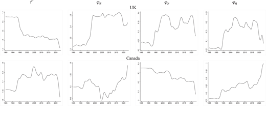
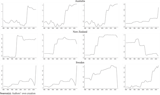
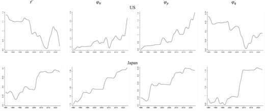
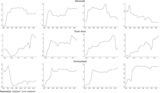
Figures 2 and 3 display the TVPs of the forward-looking standard Taylor rule for inflation targeting countries and for those with alternative monetary regimes, respectively. While some of the parameter shifts coincide with those suggested by the structural break analysis, the time-varying approach identifies more shifts than both the structural break tests or the initial visual inspection. These results imply that most countries have become more responsive to both inflation and the output gap over time. In inflation targeting countries, the adoption of inflation targeting coincides with an increase in the inflation coefficient (which is particularly sharp in the case of the UK, Canada and New Zealand), in contrast to the decrease estimated when doing sub-period analysis based on visual inspection. This shift also corresponds to a period of lower inflation and lower interest rates in all inflation targeting countries (see Figure 1). It appears that the time-varying Taylor rule captures the sharp increase in the response to inflation which occurred at the time of the adoption of the new policy rule, which was then followed by smaller parameter changes. This shift towards greater inflation stabilisation is what one would expect from monetary authorities which had made an explicit commitment to inflation targeting (Taylor, 1999a; Sergi and Hsing, 2010).
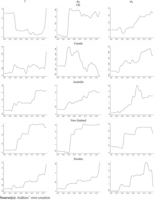
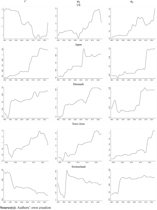
A second sharp rise in the inflation coefficient occurred after the global financial crisis in most countries. It seems that, regardless of the type of monetary regime, the crisis prompted central banks to put stronger emphasis on inflation and output stabilisation. Again this coincided with a shift towards lower inflation and policy rates in all countries (see Figure 1), which suggests that the increased emphasis on targeting inflation in the monetary policy rule was successful in reducing inflation. Consistently with the findings by Partouche (2007), our results indicate that monetary policy became more countercyclical over time, as indicated by the bigger coefficient on the output gap, which is a measure of the business cycle.
It is worth noting some important differences which can be observed between inflation targeting countries and those prioritising other monetary objectives. It appears that in the former the adoption of a new monetary rule coincides with an initial large increase in the response to inflation developments, whilst subsequently only very small changes in the inflation coefficient are implemented by monetary authorities. For instance, the reaction of inflation targeting countries to the global financial crisis was much more modest than that of countries with alternative monetary regimes, for which the inflation coefficient increased quite substantially around that time. The former showed a clear commitment to the Taylor rule over time, which might have resulted in higher central bank credibility in these countries compared to those which did not make an explicit commitment to price stabilisation and instead display greater economic discretion. However, it has to be noted that in countries with alternative monetary regimes the size of the coefficients may depend on many additional features of the economy (Taylor, 1999a). The inflation targeting framework allows countries to establish greater credibility leading to a lasting anchoring of inflation expectations. In fact, since the inflation target is a medium-term objective, inflation targeting central banks put great effort into managing inflation expectations, so that short-term deviations of inflation from the target do not result in a loss of credibility.
Next we examine in greater detail periods which exhibited large changes in the Taylor rule parameters. For instance, after 2013 there were increases in both the inflation and output coefficients in the US compared to the more inflation-focused earlier period following the adoption of an inflation targeting rule in 2012. This behaviour is consistent with the balanced approach to monetary policy advocated by Janet Yellen at the end of 2012. In the case of Australia there was a sharp decrease in the output coefficient after the global financial crisis. This finding is consistent with a more aggressive stance towards inflation coupled with a milder reaction to output, which the Reserve Bank of Australia adopted in response to the crisis (Lee et al., 2013). In general, most existing studies report a decline in the output gap coefficient for Australia over time (De Brouwer and Gilbert, 2005; Hudson and Vespignani, 2018). A sharp increase in the inflation coefficient can be observed in the case of the Swiss monetary rule in the early 1990s. During this time, the Swiss economy experienced rising inflation rates and a depreciation of the Swiss franc, which the Swiss National Bank addressed through monetary tightening. This move was inconsistent with achieving its money supply growth target of 2% and demonstrates the exercise of monetary discretion to economic developments by the monetary authority (Swiss National Bank, 2016).
It is well-known that the size of the Taylor rule coefficients strongly influences the transmission mechanism and the overall macroeconomic effects of monetary policy (Taylor, 1999a). Therefore it is crucial for central banks to understand which Taylor rule specification and parameter size is optimal at any given point in time with the aim of improving economic performance and achieving inflation stabilisation. They can learn from historical rules and economic outcomes in order to adopt a more systematic approach to monetary policy and choose optimal rules.
The standard Taylor rule is useful to assess monetary policy in closed economies, but in open economies inflation can be influenced by exchange rate changes through the exchange rate pass-through, which is why the real exchange rate should also be included in the Taylor rule. Of the countries in our sample only Switzerland and Japan are known officially to take the real exchange rate into account when setting interest rates. Figures 4 and 5 show the time-varying Taylor rule parameters for the forward-looking augmented Taylor rule which includes the real exchange rate for inflation targeting and non-targeting countries respectively. Central banks in former are now found to be more responsive to changes in the inflation as opposed to the output gap, whilst those in countries with alternative monetary regimes appear to be less responsive to either in the open-economy case. Therefore this evidence suggests differences between countries with strict inflation targeting mandates and those with discretionary monetary flexibility in the extent to which they take into account the exchange rate pass-through in their interest rate setting.
Finally, in order to investigate the possible impact of monetary surprises on the evolution of the Taylor rule parameters, in Online Appendix D we display the latter together with vertical bars corresponding to interest rate announcements with an unexpected component. In the case of Denmark, no such component could be identified in any announcement. As for the other countries, in most cases no clear linkage can be seen between unexpected interest rate announcements and shifts in the Taylor rule parameters; the exceptions are the UK and Japan, where the output gap parameter increases sharply in the aftermath of unexpected announcements in 2015, and the US, where the interest rate and inflation parameters exhibit a sizeable decrease and increase respectively after the arrival of unexpected announcements during the financial crisis, in 2008. Overall, the evidence suggests that central banks communicate their current and future policy objectives in a timely manner and that their announcements are consistent with the policy rule; as a result, monetary surprises do not appear to play a major role as drivers of the Taylor rule parameters. They can arise when the perceived responsiveness of the central bank to the economy is different from the actual one. Thus, changes in the Taylor rule parameters which are not expected by the public can be seen as monetary policy surprises. This type of imperfect information is often a cause rather than a result of the monetary surprise and can influence the transmission mechanism (Bauer and Swanson, 2023).
4.4 Robustness analysis
Following Partouche (2007), we check robustness by allowing the matrix to be non-restricted. These results are reported in Online Appendix E and confirm robustness, especially in the case of the inflation and output gap parameters. Although central banks are known to respond to anticipated inflation instead of past inflation, as a further robustness check we also estimate backward-looking Taylor rules by including the first lag of all variables. These additional results are reported in Online Appendix F for both standard and augmented Taylor rules; compared to the forward-looking Taylor rules there are only slight differences in the inflation parameter estimates, particularly in non-targeting countries. The backward-looking rules seem to be less suitable to capture major shifts (such as the introduction of the inflation targeting regime) and display greater variation in the estimated Taylor rule parameters.
5. Conclusions
This paper assesses time variation in the monetary policy rules of inflation targeting countries (the UK, Canada, Australia, New Zealand and Sweden) and others with alternative monetary regimes but known to target inflation at times (the US, Japan, Denmark, the EuroArea and Switzerland). Initially, sub-period analysis was conducted using visual inspection as well as formal break tests to identify the break dates. Then, following Partouche (2007), a TVP-GMM framework was applied to estimate TVPs in forward-looking standard and augmented Taylor rules.
The results can be summarised as follows. First, monetary policy appears to have become more averse to inflation and more responsive to the output gap over time in both inflation targeting and non-targeting countries. In the former the shift to inflation targeting coincides with a sharp increase in the inflation coefficient in the Taylor rule. For both sets of countries, a sizeable shift occurred after the global financial crisis when monetary policy became more accommodating. Second, monetary policy has become more countercyclical in all countries over time, with an increased focus on stabilisation policies since the global financial crisis. Third, there seem to be differences between countries with strict inflation targeting mandates and those with discretionary monetary flexibility in terms of the extent to which the exchange rate pass-through channel for inflation is taken into account, the former set of countries paying greater attention to it. Fourth, the TVP framework is more informative than the sub-period analysis for detecting shifts in the parameters of the Taylor rule. Finally, monetary surprises do not seem to be an important determinant of their evolution over time, which suggests a high degree of monetary policy transparency in the countries under examination. On the whole, our findings provide extensive evidence that constant parameter Taylor rules cannot capture accurately the behaviour of monetary authorities. In particular, it is clear that, following the global financial crisis, central banks have started to put greater emphasis on inflation and output stabilisation, be they inflation targeters or not.
These findings have important implications for policymakers. First, reviewing past shifts in the Taylor rule parameters alongside the historical development of inflation can provide central banks with insights into the monetary policy transmission mechanism. This can be useful to formulate appropriate monetary policies going forward. Second, policymakers should continue to ensure a high degree of transparency by clearly communicating any changes in the Taylor rule parameters to the public, since our evidence shows that this reduces the size of monetary surprises related to the monetary stance. Third, it seems that in inflation targeting countries a smaller response of the monetary rule parameters to economic shocks is required to stabilise the economy than in those with alternative regimes since in the former central banks demonstrate a consistent commitment to inflation stabilisation over time and are likely to have greater credibility. Greater transparency in inflation targeting countries reduces uncertainty regarding inflation and the conduct of monetary policy, which allows inflation expectations to be anchored more permanently. Our findings clearly reflect this distinct advantage of the inflation targeting framework.
We are grateful to two anonymous referees and to Massimiliano Caporin for helpful comments and suggestions.
Notes
The sample period includes in the case of inflation targeting countries the point when this monetary regime was adopted and for all countries several periods characterised by economic turbulence and uncertainty (such as the global financial crisis, the Covid-19 pandemic and the Russia–Ukraine conflict).
The exact inflation targets are obtained from the websites of the central banks investigated in this paper.
The filter allows to split output into a trend and a cyclical component.
References
The supplementary material for this article can be found online.
