Evaluating Potential Sources of Aggregation Bias with a Structural Optimization Model of the U.S. Forest Sector

The global climate change, forestry research and policy communities can benefit from projections of future forest land use and management based on economic models that reflect dependencies between natural resource systems, markets and policy drivers. Such tools can be used to develop future anticipated baselines, which can inform policy dialogue or investment decisions regarding activities that maintain or enhance forest carbon stocks. The myriad of methods used to project land use and GHG emissions across alternative economic futures includes simulation methods (e.g., Wear and Coulston (2015)), structural dynamic methods (Tian et al., 2018), recursive dynamic partial equilibrium methods (e.g., Forsell et al., 2016), and spatial allocation optimization frameworks (Latta et al., 2018). Structural dynamic economic models can offer distinct advantages for projecting forest carbon futures at regional and global scales, such as price endogenous land use and management decisions (Tian et al., 2018) relative to simulation approaches, but such frameworks are often built at aggregated spatial, temporal, and activity-level scales, requiring data aggregation processes to link physical forest resource or land cover data with market data (Prestele et al., 2016). Aggregating or averaging across scales is a common technique for representing physical and economic parameters in model- specific regional aggregates. Such aggregation offers operational advantages in minimizing computational processing challenges, reconciling differences in data availability at different spatial scales, and linking together resource systems with regional markets. However, there are important trade-offs associated with data aggregation for structural model development, including potential bias that can result from aggregating input data across spatial, temporal, and activity scales and thus reducing the level of heterogeneity present in the modeling system and simulation results. Reduced spatial or activity-scale data limits the amount of data heterogeneity present in a structural optimization modeling framework, moving the system further away from representing the “margin” of some key parameter set (e.g., transportation costs) and towards average regional conditions.

Aggregation bias is widely discussed in the statistical and econometric modeling literature, and techniques have been developed to correct for potential aggregation bias. However, limited work to date has explicitly evaluated aggregation bias potential in structural models. This paper seeks to fill this key gap in the forest modeling literature by highlighting potential sources of aggregation bias in baseline forestry projections using the Land Use and Resource Allocation (LURA) model, a detailed spatial allocation partial equilibrium model of the U.S. forest sector. We evaluate baseline projections of forest carbon, regional harvest levels, and other key outputs across a range of data structures representing different levels of spatial, forest type, and age-class aggregation. The spatial aggregation component relates directly to forest biomass transportation costs. The LURA framework (described in Latta et al., 2018) represents distinct transportation cost components from plots to facility (mills, electricity generation unit [EGU], and port), and from facility to facility. We evaluate aggregation bias first by averaging transportation distances and costs at a county level, a state level, and then at a regional level.

Then, we explore aggregation of forest volume characteristics across age class structure and forest type delineation. Age class aggregation includes moving from per acre volumes at an individual plot-level age class distinction to a 5- and 10-year age class aggregation (both of which are popular age-class aggregates in the forest modeling community). Age class aggregation changes both the growth dynamics and harvest rules for individual plots. Finally, we move from a forest type classification system that covers 14 individual forest types in the model to a simplistic Hardwood and Softwood delineation, which is consistent with other modeling frameworks and data-sources and the delineation for harvest levels reported from the Timber Product Output database (USDA). Forest type aggregation affects growth dynamics, harvest rules, and other management variables in the framework. Spatial, age-class, and forest type aggregation scenarios are interacted in a partial factorial experimental design to evaluate relative levels of aggregation bias across these key elements.

The advantage of our approach is that we maintain the high level of spatial resolution in the modeling framework using FIA plots as the primary supply-side simulation unit and mills, EGUs, and ports as the demand-side simulation units. Ultimately, the structure of the model remains intact, and the operational objective is still to minimize the costs of achieving national demand targets for specific forest product groups (consistent with Latta et al., 2018). However, as we aggregate across key elements of the model related to changes in demand through the shifting of transportation costs when aggregating across space, and to timber supply through changes in age class and forest type driven by forest management decisions, this approach allows us to approximate the effect of aggregation on key variables of interest (e.g., GHG emissions and harvest levels) while avoiding structural changes to the modeling framework itself. We show that aggregation across space, age class, and forest types can result in considerable variation in projected terrestrial forest carbon stocks across the United States with a 7% difference nationally and more than 25% in key regions relative to the disaggregated base model formulation.

Aggregation has long been studied in statistical analyses; particularly, econometricians are interested in accurately modeling the relationship between the individual (micro) behavior and aggregate (macro) statistics, so data from both the micro and macro level can be used for estimation and inferences about economic parameters. However, biases can arise from aggregation; Greenwood and Luloff (1979) found that aggregation bias can influence the application of the standard t test for aggregated coefficients and may change the overall fitness of a regression equation in inconsistent ways. Additionally, Luloff and Greenwood (1980) found coefficients switching signs and magnitude with the sign switching remaining statistically significant when aggregation was included across a sample. These, and other findings (see Theil, 1954; Boot and G. M., 1960; Orcutt et al., 1968; Gupta, 1971; Sasaki, 1978), led to the derivation of statistical test which could be used to measure aggregation biases, such as in Pesaran et al. (1989), and Lee et al. (1990).

In structural models, aggregation can also be thought about as using micro level data to represent macro level responses to economic conditions. Aggregation bias is also present in structural models, as shown in Foroni and Marcellino (2014), which applies a dynamic stochastic general equilibrium model (DSGE) to show that potential biases from temporal aggregation can be large in empirical models. Using the Global Trade Analysis Project (GTAP) modeling systems, Brockmeier and Bektasoglu (2014) analyze and compare the effects that data aggregation and model structure have on results. Brockmeier and Bektasoglu (2014) apply both general equilibrium (GE) and partial equilibrium (PE) versions of GTAP, as well as aggregated and disaggregated versions of the input data. Results show that data aggregation, especially related to competition and tariffs, has a larger effect on model outcome than model structure. Charteris and Winchester (2010) use a computable general equilibrium model (CGE) to see the impact of dairy disaggregation and joint production on trade liberalization outcomes. This study shows that aggregation can lead to misleading results if joint production is not accounted, such as lower rates of exportation, reduced economic output, and lower welfare effects due to the substitution effect on the consumption side. Applying the GTAP model Grant et al. (2007) investigate the effects of reduced trade barriers of the U.S. dairy sector and find that an aggregated version results in an underestimation of trade flows compared to the disaggregated version, and production is reduced (similar to Charteris and Winchester, 2010), but relatively consistent results surrounding total welfare across the models. Narayanan et al. (2010) compared PE, GE, and a combined PE-GE model to estimate the welfare effects of the Indian automotive industry under reduced trade barriers. They found that when data inputs are aggregated, total imports increase, overall prices change slightly, and a relatively small change in total welfare.

The effects of spatial aggregation have been researched in the civil engineering field with respect to transportation as well. Jeon et al. (2012) showed that using an aggregated Traffic Analysis Zone structure and network model with aggregated regions can still produce results within a reasonable range of error requiring less time and costs of the analysis. Varejão and Portugal (2007) used historical labor data to estimate labor demand functions across varying levels of spatial and temporal aggregations. Data aggregated from the quarterly level to the annual level resulted in estimates of longer adjustment lag time between reaching a market clearing steady state, that is, an upward bias in the estimated coefficient of the lagged dependent variable (Varejão and Portugal, 2007). When data was aggregated spatially, from individual establishment level to industry level, the estimated coefficients had the expected signs, but as data was aggregated to larger industries, the effects of lags and coefficients were more reasonable. These results demonstrate that the most disaggregated estimates were less reliable than higher levels of spatial aggregation. Additionally, several studies have evaluated the “zoning effect” and its implications multivariate regression parameter estimation (Amrhein & Reynolds, 1976, 1996, 1997; Reynolds & Amrhein, 1998; Fotheringham and Wong, 1991; and Openshaw and Taylor, 1979). The zoning effect is created by aggregating statistics across some partition created through some decision-making process, an example of this is aggregating individuals up to the census track level (Reynolds & Amrhein, 1998).

Structural models of the forest sector rely on a wide range of aggregating assumptions in order to simplify both the input data requirements of models, and the computational rigor of solving a large optimization model. Table 1 provides an overview of recent modeling studies in the forest economics domain, focusing primarily on studies in the projections and climate/bioenergy policy domains in which developing robust baseline forest carbon projections is often a primary objective. Economic modeling approaches highlighted in Table 1 include structural dynamic models (GTM, FASOMGHG), recursive dynamic global partial equilibrium frameworks (GFPM, GLOBIOM), spatial allocation optimization (LURA), an integrated assessment model (GCAM), and a regional partial equilibrium framework (SRTS). Models vary significantly in how forest sector activities are aggregated by region, time-scale (or simulation step), age-class structure, and forest type delineation. Table 1 focuses on aggregation of U.S. forest sector components—for global models, frameworks may have different aggregation approaches for different regions. This table shows that most existing economic models used for projections analysis aggregate to at least a 5-year age class structure with regional aggregates for supply-side representation. Some frameworks also use a high-level of aggregation to distinguish different forest types.

This analysis applies the Land Use and Resource Allocation Model. LURA is a recursive dynamic, spatial allocation model of the US forest sector (Latta et al., 2018; Martinkus et al., 2017). The LURA framework efficiently allocates forest resources to either match exogenous demand targets over time for different forest products (as in this analysis) or to match exogenously-defined harvest levels from other projections models (e.g., Latta et al., 2018), which uses key macroeconomic and energy market drivers, such as GDP, housing starts, and diesel prices, to project future demand targets for 22 individual forest products.

Forest biomass is supplied at the plot-level, based on data from the Forest Inventory and Analysis 2015 (FIA). The FIA plots are part of the national inventory of forests for the United States. In total, 150,350 forest plots are included in LURA with information on condition classes,¹ eco-provinces (Cleland et al., 2007), site classes, forest type, age class, management intensities, and ownership characteristics for each plot. Representative annual growth rates are calculated for each forest type, land classification, and eco-province combination (a further explanation can be found in the supplement of this manuscript and in Latta et al., 2018). The harvest decision is based on minimizing the transportation costs of harvest logs to mills with available capacity, and travel of final goods from mills to demand ports.

Aggregation scenarios in this analysis include spatial, forest type, and age class aggregations; as well as interactions between key aggregation categories. Three different aggregation levels were implemented to examine the effects of aggregation on results for both natural and economic systems within the same modeling framework. The first level compares results across different spatial aggregates moving from individual plots, to counties, to states, and finally to major market regions as represented in the U.S. Forest and Agricultural Sector Optimization Model with Greenhouse Gases (FASOMGHG) framework as summarized in Baker et al. (2010), Latta et al. (2013), and Cai et al. (2018). Spatial aggregation directly affects the travel cost associated with moving harvested logs to mills, intermediate wood products to mills and ports, and final products to demand centers such as ports. We find through our aggregation processes that in regions with highly developed forestry industries, overall travel costs decline under spatial aggregation; conversely, regions with limited infrastructure see travel costs increase with spatial aggregation as large areas of forestland exist far from mills. The second aggregation source moves from plot specific age-class delineations (pulling ages directly from the FIA dataset for each plot) to 5-year age classes across each spatial aggregation level. The final source of aggregation considers a 10-year age class across each spatial level, while also aggregating from the original 14 forest types to two representative forests (hardwoods and softwoods). Our choice of aggregation across plot ages to age classes as well as from specific forest stand types to generalized hardwood and softwood categories changes the per-acre volume level, growth rate, yield, and harvesting costs from the margin to the average which affects harvesting decisions, production of harvested wood products, and carbon storage.

The following sections provide additional detail on these aggregation procedures and how they impact model functionality and resulting outcomes by shifting the basic economics of the system and forest management decisions.

The degree of spatial aggregation of a model directly affects resource supply, moving it further from spatial heterogeneity and thus marginal nature of supply to one more reflective of constant averages. Our spatial aggregation scenarios in LURA first require a weighted average representative plot location (latitude and longitude) to be created for each spatial aggregate. We then conduct the same level of aggregation for demand points (forest product mill, electricity generation unit [EGU], or port) for each of the forest product classifications. The scenario-specific locations are then run through the LURA transportation cost algorithms (see Latta et al., 2018) to determine transportation distances and costs.

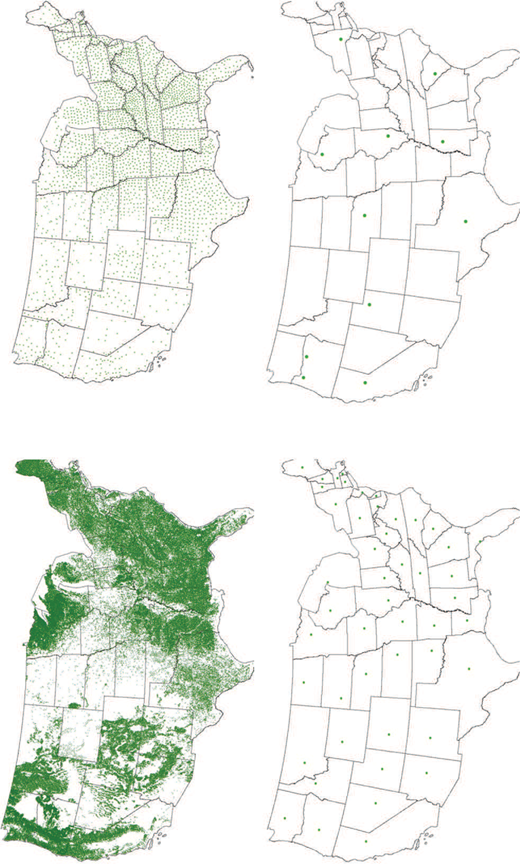
In the base (labeled Plot in Figure 1) scenario transportation distances and hauling costs are calculated independently for each combination of 150,350 plot and more than 3000 demand point locations, given an assumed energy price projection (in this case we assume 2018 Annual Energy Outlook Reference Case diesel prices). Thus, the plot scenario results in the most spatially heterogenous cost estimates yielding smooth upward-sloping marginal transportation cost functions. For counties (labeled County), we first calculate the weighted average centroid location of forest plots within each county of the lower 48 states then repeat the procedure for the forest product manufacturing facilities. Next, transportation distances and associated hauling costs are recalculated for this generic plot location. This procedure is replicated for state (labeled State) and regional (labeled Regional) versions of the model as well. Subsequent model simulations continue to manage individual plots, but spatial heterogeneity in transportation costs decreases with each level of aggregation. As spatial aggregation occurs, regions with a limited number of mills end up with relatively large average transportation costs compared to regions with a large numbers of mills. These regions with less existing forest product manufacturing infrastructure have relatively steep marginal cost curves, and when travel distance (i.e., a proxy for transportation costs) are averaged across the entire region, these plots are no longer cost competitive for mills within region or in neighboring regions. Additionally, spatial aggregation directly effects a models ability to efficient allocate intra-regional transfers of products. In a plot level analysis, each plot is able to ship products to the closest, economically feasible, mill no matter what county, state, or region that mill is in. This allows for the marginal transportation cost for many plots to remain low. As travel distances from plots to mills are averaged across large spatial expanses these low marginal costs begin to increase for plots which previously shipped biomass to mills in other regions. Figure 1 shows Plot, County, State, and Region forest resource locations, providing a visual illustration of the degree of spatial aggregation associated with each scenario.

Next, we consider alternative age class structures in the model, aggregating from the single-year age class delineation used in the base LURA model to 5-year and 10-year age class aggregates. Specifically, we take the LURA forest plot per-acre volumes representative of a given stand age and group plots into common aggregates for five-year (0–4, 5–9, 10–14, etc.) and 10-year (0–9, 10–19, 20–29, etc.) age classes for which we calculate an area-weighted peracre volume. This process reduces the heterogeneity in FIA-reported stocking levels present in the base model, as plots within a specific age-class group are aggregated and assigned an initial stocking rate that averages across all plots by forest type and site class.

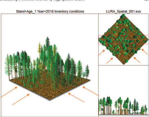
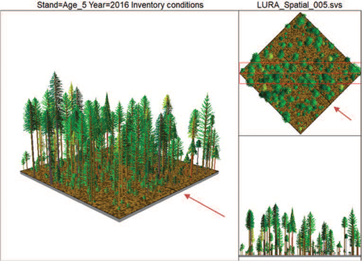
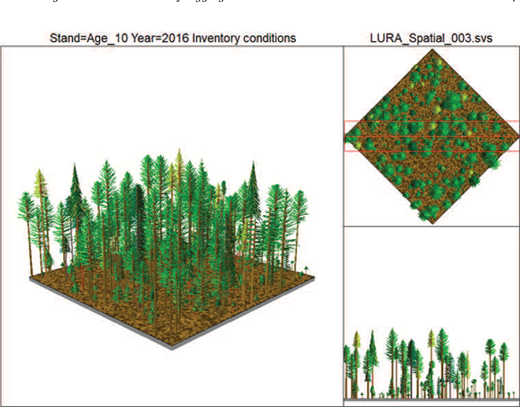
The SVS info graphics in Figures 2, 3, and 4 illustrate this concept through a visual representation of a group of plots ranging from 60–69 years in age for an FIA sample of Douglas-fir plots in the Interior West region. The left panel of each figure shows a single-year age-class structure, with nine representative plots (represented by black boxes) showing average stocking density for plots at a given age class. Figure 2 demonstrates the level of heterogeneity present in initial inventory conditions for a single forest type and region combination. Heterogeneity across a plot can be caused by regeneration success, previous disturbance, management, or other ecological processes. This heterogeneity is captured in the representative nine plots seen in the top right panel of this figure, which provides a bird’s-eye view of the simulated plots. The horizontal perspective of this plot grouping (lower right-hand side) also shows spatially heterogeneous initial inventory conditions from this data query.

Figure 3 shows the same visual, with only two representative plots and assuming two 5-year age class aggregates within the 60–69 year window (60–64 years and 65–69 years, respectively). This aggregation shows the process of moving from nine representative plots with the one-year age class structure to two plots that average across groupings of those original nine plots that fall within the 5-year aggregates. Thus, the same original set of trees in the 1-year age class SVS info graphic are re-shuffled from nine representative plots to two, which reduces heterogeneity in initial inventory. The 5-year age class aggregation also offers some degree of heterogeneity in inventory, as demonstrated visually in the discernible difference between the upper/right- hand side representative plots and those on the left, but the difference is less extreme than for the single-year age class aggregation shown in Figure 2. Figure 4 illustrates a 10-year aggregation (60–69), which results in an even more homogenous initial inventory as the original nine subplots are now represented by a single block with an average stocking density across the original nine.

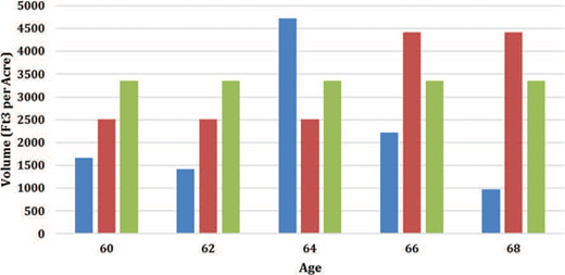
Expanding this example, Figure 5 illustrates the importance of age class delineation on initial inventory parameters for representative plots of a certain forest type/region combination. Again, using Douglas-fir plots in the Interior West region for this illustrative example, Figure 5 compares initial inventory cubic volume per acre across the different age class structures demonstrating how initial inventories compare to aggregates across the scenarios. Representative 1-year age class (Plot scenario formulation) for different plots results in inventory conditions that vary substantially across years, while a 5-year aggregation shows two distinct inventory levels and the 10-year age-class averages out these low- and high-end stocking levels in the sample and provides a consistent single stocking level for the plots within this age class, significantly reducing the heterogeneity inherent in the system. This averaging, or smoothing of conditions, affects harvest costs (determined by per-acre removals) and thus the harvest decision within the model.

Finally, we consider alternative forest type aggregates. The basic forest representation of LURA includes 14 primary forest types² reflecting the diversity of species compositions in the forests of the conterminous U.S. This study adds a scenario formulation that consolidates these forest types into two broad Hardwood and Softwood classifications. This aggregation reduces the level of detail by limiting the model’s ability to achieve higher relative yields at additional costs with plantation forest systems. Furthermore, this level of aggregation over-simplifies the inventory stocking assumptions in the model for existing forest plots in the FIA database by averaging out productivity and carbon storage differences across species. From an economic perspective it also limits the harvest choices to species averages thereby eliminating the option of targeting plots with high proportions of relevant merchantable products such as softwood sawlogs or hardwood pulpwood.

In a broad sense, the spatial aggregation scenarios can be considered a focus on the effects of transportation costs, the age class aggregations on the effects of harvest costs, and the forest type aggregations on the effects of log primary forest merchantability. The resulting suite of scenarios thus is designed to provide a rich overview of a wide range of potential aggregation bias issues. Table 2 describes that various scenarios utilized in this analysis and how each varies levels of aggregation in spatial and activity-scale components.

Aggregating distances to mills or other final demand points shifts representation of key economic parameters (e.g., transportation costs) from an approximate marginal cost specification closer to average considerations. With regional average transportation cost parameters, even if biomass supply is represented at a plot level, a forest modeling framework will be agnostic between harvesting two plots with similar physical characteristics, even if the plots are (i.e.) 20 and 50 km away from a demand point.

Somewhat surprisingly, however, our results indicate that when implemented, spatial aggregation has only a modest impact on aggregate forest carbon accumulation at a national scale (Tables 3 and 4). Table 3 presents the total estimated CO₂ stored in the United States forest sector in each scenario at two points in time, 2026, and 2036, and Table 4 shows the percent difference in projected CO₂ storage across different scenario assumptions relative to the base model formulation (1-year age class, all forest types, and plot- level transportation cost assumptions). Results show a negligible difference in carbon storage when moving from plot to county-level aggregates (approx- imately 0% in all time steps). Aggregating to the state-level decreases CO₂ stocks slightly and this difference grows over time but represents less than a one-percent difference in projected carbon stocks relative to the base formulation for all time periods. Regional aggregation of transportation distances and costs has the most meaningful impact on carbon stocks, resulting in a net increase in projected carbon relative to the base formulation of approximately 1% over the simulation horizon.

The change in aggregate carbon storage is a result of shifting regional harvest patterns. Cumulative removals decrease overall under the regional aggregation scenario relative to other spatial considerations, which boost carbon stocks in regions with less forest sector activity overall (e.g., the Corn Belt and Pacific Southwest regions). With higher transportation costs, harvest patterns shift to regions with greater existing mill capacity and lower relative transportation costs. Mill residual utilization also increases, resulting in a forest product sector that is more confined to the Southeast, South Central, and Pacific Northwest regions. LURA includes assumptions governing the supply of industrial byproducts from forest product manufacturing (e.g., bark, shavings, and sawdust) and this biomass can be utilized as an energy input or to produce other products (e.g., pulp).³ As relative costs increase with aggregation and production shifts to regions where lumber and pulp mills are co-located (or are in close proximity), a greater proportion of lumber mill residual biomass is utilized by pulp and paper mills. This result occurs in part due to the loss of spatial heterogeneity when averaging across regions; when modeled at the plot-level, regions with few mills still have relatively large amounts of forestland within a small supply radius to meet demand for harvested logs. As aggregation in these regions occur, these low-distance plots are no longer modeled, instead all plots within the region have the same average distance to a mill. By moving from the margin to the average, productive forest areas in regions with few mills are ignored, exacerbating the competitive advantage of regions such as the southeast and northwest.

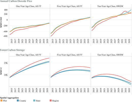
While projected national carbon stocks show minimal overall changes with higher levels of spatial aggregation (i.e., county, state, and regional) versus the base model formulation, the projected flux and carbon stocks vary more with the age class and forest type aggregation scenarios. Shifting from a 1-year to a 5-year age class distribution with a plot-level model formulation results in approximately 1.5% less carbon storage by 2028 and 3.4% less carbon by the 2036 simulation period. Projected CO₂ fluxes (shown in Figure 6), which remain negative when aggregating across space, convert from net sink to emissions source with a 5-year age class aggregation, and this switch occurs late in the simulation horizon [after the 2030 simulation period—consistent with projections reported in Latta et al. (2018) and Wear and Coulston (2015)]. Reverting from sink to source of emissions over a 20-year flux indicates that age-class aggregation represents an important source of potential bias with the key policy implication that projected national emissions level (economy-wide) would be higher in the presence of this aggregation as the LULUCF flux has historically been an important annual sink for the U.S. (EPA, 2018).

Aggregating to a 10-year time step and with forest type aggregation (two types instead of 14) results in projected carbon stocks that are approximately 8% less than the base model formulation and the projected carbon flux reverts from sink to source early in the simulation horizon (after the 2020 simulation step). Thus, U.S. forest carbon stocks are declining for the bulk of the simulation timeframe. While other recent projections that rely on modeling frameworks with a decadal age-class structure representation have projected a continuing sink for U.S. forests (Tian et al., 2018), we show different results (that is, we find a more rapid decline in carbon accumulation with age-class aggregation). The difference in the overall sign in the projected flux change between Tian et al. (2018) and this study can be explained by the lack of endogenous land use and management options in LURA. But our results do show potential bias in age-class aggregation, which can shift both initial carbon stock conditions due to differences in initial inventories, as well as the shape of the flux projection as economic criteria regarding “when” to harvest can change for all plots.

Projected national changes in carbon stocks are less than 10% over the simulation timeframe for all sources of aggregation considered in this study, which is relatively small in percentage terms, but represents a meaningful portion of U.S. terrestrial carbon storage. However, fluxes vary significantly, which has important implications for policy makers and other practitioners that seek to establish baseline projections of future forest or land use sector emissions. For context, the difference in baseline flux projections presented in this analysis is larger than the differences in LURA-derived emissions projections across macroeconomic scenarios presented in Latta et al. (2018), but not as large as the differences in projected emissions flux presented in Wear and Coulston (2015) and Tian et al. (2018), and the latter two studies rely on very different underlying modeling methodologies.

In addition to shifting initial inventory conditions, national and regional changes in harvest patterns are key drivers of projected carbon outcomes. Regional differences in projected harvests are driven in part by the geopolitical boundaries and relative forest density between different regions, which has implications for transportation cost calculation as the model formulation is aggregated from plot level to other spatial aggregates. For instance, in the eastern United States, counties and even some states are relatively small compared to the west and mid-west regions, and thus aggregation from plot- level transportation cost parameters to county- or state-level has little effect. Projected harvest levels are similar for the plot- and county-level model formulation, regardless of age-class or species aggregation considerations (Tables 5 and 6). Consistent with the slight decrease in projected carbon stocks, aggregate harvests increase slightly for the state-level scenarios (less than one percent). Projected harvests for the regional formulation (with a one-year age class distribution and heterogeneous forest types) are approximately 6%–10% lower than under the plot-based model formulation, which is again consistent with the projected change in carbon stocks presented in Tables 3 and 4. The regional aggregation induces large changes in plot-level transportation cost considerations, making forest harvests much less economical in regions with low levels of forest density.

The 5-year age class aggregation also shifts cumulative national harvest levels – increasing in the first five years, but then decreasing over the remaining intervals for the plot, county, and state formulations. The net change in projected harvests is small (less than one percent) for all Age5FT scenarios relative to the base formulation except for the regional aggregate (which sees a decrease in harvests of approximately 9% relative to the plot-level formulation).

The Age10HWSW scenarios show a long-term increase in cumulative harvests for the plot, county, and state scenarios relative to the base formulation, but this effect is relatively small overall (2%–4%). Under the regional formulation for Age10HWSW, total cumulative harvests decline approximately 4% by the 2036 simulation period. This change in directionality between the regional aggregation and plot, county and state aggregations is surprising. Even when aggregating across age class, and forest type the projected harvest levels are consistent, but once plots are aggregated across large regions the results are inconsistent. As mentioned previously, regional aggregation moves transportation costs from the margin to an average which increases the costs of producing wood products using primary logs. This forces the model to rely more heavily on utilizing bioproducts and residues to produce things like paper and boards. Overall, aggregation has only a small effect on harvesting decisions in this frame- work, but aggregation more greatly effects projections of forest carbon storage.

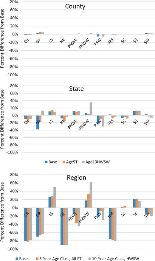
Not all forest types are affected equally across the US across aggregation scenarios. Overall, the average travel distance of hardwood harvest is much more variable compared to softwood harvests. This is driven in part by less forest density for traditional hardwood stands as these stands typically require longer growing intervals for harvest, which limits the available alternative plots with viable amounts of biomass. When performing regional analysis, differences in projected carbon and timber product supply across various levels of spatial and activity-level aggregation can lead to very different conclusions. At the state and regional aggregations, the effects are much larger in magnitude, resulting in large cumulative reductions in harvesting in the Northeast, Corn Belt, Rocky Mountains, and Great Plains, with a decline of 90%, 81%, 76%, and 70% in harvest levels (respectively) when moving from plot level locations to a regional average locations respectively (Figure 7). While these effects are large in percentage terms, it is important to note that these regions, in particular the Corn Belt and Great Plains, play a relatively small role in the national forest product supply. Additionally, in the plot-based model, the Corn Belt is sending over 30% of its harvested logs to other regions for processing. When travel distances are averaged across the entire region, plots which may be near the border of a region, and closer to mills in other regions are going to experience a greater impact in costs. If aggregation shifts cost structures and regional comparative advantages further in favor of regions such as the Southeast, South Central, then an efficient solution is to reduce harvests and concentrate product mill capacity in these regions, which we find.

Differences in cumulative harvests for the regional aggregate scenarios are driven by a spatial reallocation of forest sector activity out of larger regions with relatively low forest density and high aggregated transportation costs to more traditional forest sector regions. The Southeast, South Central, and Pacific Northwest (West) regions all see meaningful increases in cumulative harvests under the regional aggregate scenarios, and this effect is amplified when age-class structure and forest type considerations are also aggregated. This reallocation occurs as higher costs and less heterogeneity in plot-level characteristics shift the domestic regional comparative advantage of forest product activity further in favor of highly productive regions. Furthermore, the Lake States region, which is a relatively small region but is endowed with existing mill infrastructures and high levels of forest density sees increased projected harvest levels for the regional scenarios relative to plot-based locations, with increases of more than 20% for all aggregation scenarios relative to the base formulation. Thus, at higher levels of transportation cost and plot characteristic aggregation, there is a distinct shift to regions with existing infrastructure, which artificially de-emphasizes existing forest sector activity in regions such as the Corn Belt or Pacific Southwest in lieu of regions with increased comparative advantage under new cost structures created by data aggregation processes. Our hypothesis is that this type of aggregation bias is evident in other modeling frameworks as well that rely on large regional delineations, but models that are not based on spatially explicit units may not offer the ability to directly test for spatial aggregation bias.

Furthermore, while national harvest levels decline under regional aggregation, exogenous demand targets for all forest product categories are still met as a higher total proportion of harvested logs are utilized, logging residue collection and use increases, and use of mill residuals increases. Higher levels of residue utilization results in an overall decrease in the amount of new harvest that is required to meet exogeneous demand. Our results show that in the regionally aggregated model an increased reliance on byproducts occurs to meet demand which leads to an overall reduction in cumulative harvest by 8.4% by 2028 compared to the plot-based model, even with large regional shifts in harvest patterns.

Aggregation across space, time, and forest types also impacts total harvest levels and the average yield per acre, or the relative intensity of harvests. At the most disaggregated level, average volume harvested per acre over the entire time horizon was 3.2 thousand ft³/acre for the plot-based scenario, while in the fully aggregated model yields are 2.6 thousand ft³/acre. This is due mainly to the shift in initial conditions associated with moving from 14 individual forest types to only 2-forest types. The initial forest inventory in both models is the same, however, because the 2-forest type model has averaged-out the fast-growing plantation forest types, the growth rate of forests in the United States declines relative to the baseline model. This leads to a high rate of harvest on these “overstocked” forests in early periods with the resulting forest regrowth experiencing lower growth rates.

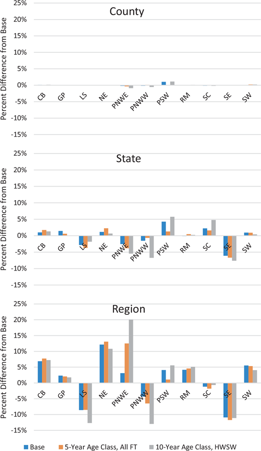
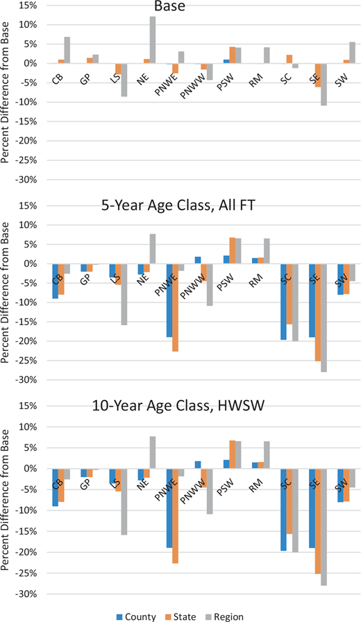
Carbon stocks also vary substantially by primary market region (Figure 8), in particular at regional aggregates and with higher levels of age-class and product aggregation. The Southeast and Southcentral regions show the largest decrease in projected carbon storage with decreases in carbon storage of 0.50 Gt CO₂ and 0.49 Gt CO₂, respectively, relative to the base model formulation and the Age5FT formulation at the plot level, and this difference grows for the Age10HWSW aggregation (1.5 Gt CO₂ and 1.1 Gt CO₂ respectively). Aggregation to the regional level induces the largest increases in regional carbon stocks, with the Northeast, Rocky Mountain, and Corn Belt all experiencing large changes (0.97 Gt CO₂, 0.3 Gt CO₂, and 0.20 Gt CO₂ respectively), while regions such as the Southeast, Lake States, and Pacific Northwest (West) see the greatest decreases in carbon stocks. The Southeast in particular sees a large decrease in carbon, reverting from a strong net sink to a large net source of emissions by 2036 for the state and regional scenarios and under the Age10HWSW formulation.

These regions include large areas of highly productive plantation forests, and aggregation leads to an “averaging out” of these productive ecosystems, particularly for the Age10HWSW scenario formulation. This omission of plantation forests within the model limits the ability of the forest sector to provide fast-growing, high-quality biomass. This in turn forces an increase in the harvested area without a commensurate regrowth in carbon under the influence of management. Forest management considerations are critical in understanding and projecting the forest carbon balance (Tian et al., 2018), so averaging out important management characteristics of different forest types has important implications for regional carbon flux (and stock) projections in regions that rely heavily on management interventions to improve productivity. Projected forest carbon flux in the Southeast region under the highest level of aggregation (regional, Age10HWSW) indicates a net emissions source of 0.56 Gt CO₂ annually, and more than a 25% reduction in projected carbon stocks by 2036 (Figure 9). Similarly, the South Central region sees more than a 20% reduction in projected carbon stocks for the most aggregated model formulation relative to the base formulation. This result suggests that regional stakeholders should be cautious when interpreting regional projections from highly aggregated national forest sector models, for the potential for biased results exists.

The prevalence of biophysical-economic modeling used to establish baseline projections of market or environmental variables to inform policy decisions will continue to expand, and there is a growing literature that seeks to explore the implications of alternative modeling techniques on projections outcomes, particularly for energy, agriculture, and land use systems and with a growing emphasis on forestry. For forest sector projections modeling, it is also important to understand the implications of various data aggregation techniques on projection outcomes. Using the LURA framework, this study attempts to quantify the effects that aggregation can have on structural model projections by varying the level of aggregation across supply/transportation cost components, forest management considerations, and forest types.

This analysis shows that projections of standing timber vary at the national level by less than 5% over a twenty-year time frame with spatial aggregation, which is small overall, indicating limited potential bias of spatial aggregation when modeled results are evaluated at national scales. However, we find much greater variation in projected harvest and carbon results at the regional level as the regional comparative advantage of forest product supply shifts to regions with high relative forest density and existing mill infrastructure. This effect is the result of a model-derived change in comparative advantage that reinforces a spatial redistribution of production activities due to economic data aggregation, thus introducing potential bias in regional projections results.

The largest source of variation in projected carbon and harvests is aggregation across both forest types and age classes (Age10HWSW). The implication of this result is that even models that account for spatial heterogeneity in transportation costs can suffer from aggregation bias if activity definitions such as forest types and age class structures are averaged. Under the Age10HWSW model formulation, projected carbon storage in the United States declines by almost 8% over a twenty-year simulation horizon. Regional results are also greatly impacted by age class and forest type aggregation. Specifically, we find that the largest affects occur in the highly productive regions such as the Southeast, South Central, and Pacific Northwest with projections of carbon storage declining by as much as 28% relative to the most disaggregated model formulation. This reduction in carbon occurs in the absence of management intensification or investment in forest resources at the extensive margin – such investments are not endogenous components in this version of the LURA model. With shifting cost structures and regional harvest patterns, there would be a large market incentive to invest in management techniques that increase overall productivity (e.g., planting), consistent with findings in Tian et al. (2018). However, this result also suggests that modeling frameworks that aggregate over space and activity sets could see biased levels of forest resource investment in productive regions with relatively lower cost structures following aggregation of input data, and this can also influence projected carbon outcomes. Further research is needed to assess whether this directionality is consistent across other modeling frameworks in order to better understand the potential sources of bias inherent in data aggregation processes for structural models.

Finally, while it is not always feasible to use the most disaggregated level of data due to lack of economic data at higher spatial resolution or limited computing power; it is vital that the potential biases associated with varying types of aggregation be explored and taken into consideration when developing regional carbon stock projections from national or global systems models to use in different policy or investment contexts.