


Backward erosion piping (BEP), a form of internal soil erosion, often threatens the safety of dykes built on alluvial deposits. To reduce the risk of dyke failure due to piping, reliable and cost-effective mitigation measures are essential. For the first time, this paper proposes the use of nature-inspired low-permeability barriers to mitigate BEP. The potential of this novel solution is demonstrated in a series of laboratory physical tests. Low-permeability barriers are created by mixing sand either with aluminium–organic matter flocs, or clay. The results show that both kinds of barriers can significantly inhibit pipe progression and intercept the erosion channels. The hydraulic gradients required for pipes to reach the barrier are significantly higher than the critical gradient measured in the absence of barriers, ranging from 2·2 to 7·4 times greater than those in sand alone. The associated mitigating mechanisms include the dissipation of flow energy, resistance to internal erosion due to pore space clogging and prevention of sand fluidisation. The mitigating effect is affected by the reduction of hydraulic conductivity, the depths and the heterogeneity of barriers. The findings of this experimental work provide guidance for the design of low-permeability barriers in practice and contribute to the development of numerical models for BEP.
NOTATION
- A
cross-sectional area of the sand sample (m2)
- Dr,sand
relative density of the background sand in the sample
- dx
grain size for which x% of the sample’s mass is smaller than (m)
- Gtotal
total hydraulic gradient (Gtotal = ΔH/Ls)
- Hc
critical head drop (m)
- h
local hydraulic head at piezometer points (m)
- Ksand
hydraulic conductivity of the background sand in the sample (m/s)
- Ls
distance from the inlet to the outlet (m)
- l*
normalised pipe length by the distance from the inlet to the outlet
- M
total number of piezometers used in the calculation of mean absolute error
- nsand
porosity of the background sand in the sample
- Q
measured mass flow rate by the scale (g/s)
- ΔH
total hydraulic head drop applied to the sample (m/s)
- η
local head drop ratio at piezometer points (η = h/ΔH)
- vout
outflow Darcy velocity
- ρ
density of water (kg/m3)
INTRODUCTION
Backward erosion piping (BEP) is an internal erosion mechanism in which channels are formed in soils beneath water-retaining structures as a result of soil removal by the action of water (Van Beek, 2015). BEP usually occurs below dykes during flood events when the average hydraulic gradient across the dyke exceeds its normal level. Alluvial geological conditions with layers of sand below a cohesive blanket of clay or peat are particularly prone to BEP. Therefore, BEP constitutes a critical failure mechanism of dykes in alluvial deposits, threatening the flood defence systems. Numerous dyke failures reported in the literature are attributed to BEP (Danka & Zhang, 2015).
Early research based on case studies introduced fundamental concepts in the analysis of BEP. Bligh (1910) established an empirical relationship between the critical head difference Hc causing piping failures of dykes and the seepage length Ls (defined as the length between the upstream entry and the downstream exit of water). Lane (1935) analysed the seepage length necessary to prevent failures from BEP, attributing larger resistance to vertical components along the seepage path than horizontal components. Later, experiments added insights into understanding the mechanisms of BEP. Sellmeijer (1988) examined the critical gradient (defined as Hc/Ls) in laboratory tests, which contributed to the development of a mathematical model for the estimation of the critical gradient. More recently, it was shown that two processes are critical before BEP can lead to structural failure: pipe initiation (Van Beek et al., 2014; Fleshman & Rice, 2014) and pipe progression (Van Beek et al., 2015; Xiao et al., 2019; Pol et al., 2022). The findings suggested that the increase of the local hydraulic gradient at the erosion zone propelled both the initiation and progression of the pipes. To gain a deeper insight into the local fluid–solid interaction, micro-scale numerical models, such as the coupled lattice Boltzmann/discrete-element model (Lominé et al., 2013), can help determine the hydrodynamic forces and reveal grain detachment under piping erosion.
Various solutions have been developed to mitigate BEP. The filter-drain system can prevent the movement of base soils and direct the seepage flow to the surface. Another typical strategy is to block the pipe. Zhou (2006) and Zhou et al. (2007) investigated the characteristics of pipe progression obstructed by the cut-off wall and the effect of the wall position on the critical gradient. They found that the cut-off wall can largely raise the critical gradient. When the critical gradient was reached, a vertical pipe developed along the downstream side of the wall due to sand fluidisation, circumvented the wall and progressed upstream until failure. This phenomenon was also observed by Achmus & Mansour (2006) and Okajima & Tanaka (2008), and was later demonstrated by numerical simulations (Zhou et al., 2012; Wang et al., 2014). Förster et al. (2015) tested the effectiveness of a vertically inserted geotextile against BEP. Rosenbrand et al. (2022b) proposed using a coarse sand barrier to prevent pipe progression, as this kind of barrier reduces the hydraulic load acting on the pipe tip when it reaches the barrier. Rosenbrand et al. (2022a) derived a local, scale-independent, strength criterion for the coarse sand barrier, which can be applied for design by numerical modelling.
This research proposes a novel nature-based measure to mitigate BEP, namely, low-permeability barriers created by applying aluminium–organic matter (Al–OM) flocculation (Zhou, 2020). The inspiration of this technique originates from the formation of podzol soils in nature. During podzolisation, the reaction of organic matter with polyvalent metals, such as iron and aluminium, produces organometallic complexes, which can flocculate under favourable environmental conditions (Blume et al., 2016). The sizes of these flocs range from 10 μm (Scheel et al., 2008) to 1000 μm (Jarvis et al., 2005) in magnitude. This broad size range endows the potential of the flocs to clog the pore throats and, consequently, reduce soil permeability. A series of field tests successfully created low-permeability barriers in situ through injection and identified two injection methods: separate injection of Al–OM (Zhou et al., 2019) and direct injection of Al–OM flocs (Zhou et al., 2022). Furthermore, increasing the fine content in soils can enhance the resistance against internal erosion (Bendahmane et al., 2008; Richards & Reddy, 2012).
Low-permeability barriers created by Al–OM flocculation have advantages in mitigating BEP. First, the low-permeability barrier can reduce the hydraulic gradient near the pipe tip by largely dissipating the hydraulic head within the barrier (Fig. 1). This allows mitigation of pipe progression even before the pipe reaches the barrier and avoids relying on the strength of barrier materials. Second, the horizontal flow through the barriers could inhibit the development of vertical pipes due to sand fluidisation along the downstream boundary of the barriers, observed in tests and simulations of impermeable barriers (Zhou et al., 2007; Achmus & Mansour, 2006; Okajima & Tanaka, 2008; Zhou et al., 2012;Wang et al., 2014). Third, the construction of barriers is less disruptive in the field by the injection technique and more economical as well as ecologically friendly. These features are favourable for large-scale application.
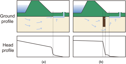
Impact of a low-permeability barrier on backward erosion piping (BEP): (a) piping without a barrier; (b) piping mitigated by a low-permeability barrier
Impact of a low-permeability barrier on backward erosion piping (BEP): (a) piping without a barrier; (b) piping mitigated by a low-permeability barrier
This paper presents a series of laboratory physical tests that demonstrate the potential of low-permeability barriers to mitigate BEP. The objectives of these tests are to answer two questions, namely, whether low-permeability barriers can inhibit pipe progression, and to what extent low-permeability barriers can resist internal erosion. As a first step towards the creation of large-scale barriers through injection of Al–OM flocs, small-scale low-permeability barriers are made by manual preparation procedures in this research. Al–OM flocs are mixed with sand to create sand–floc barriers. Since clayey sand exhibits lower permeability than pure sand (Revil & Cathles, 1999), it is used to fabricate clayey barriers. The comparison between sand–floc barriers and clayey barriers can verify if sand–floc barriers indeed act as low-permeability barriers. The tests with pure sand serve as the reference tests for the barrier experiments. Pipe progression is observed in the three types of tests and analysed together with measurement data. The tests indicate the underlying mechanisms of barriers on mitigating piping. The influential factors on mitigating effects are assessed, including hydraulic conductivity, depths and heterogeneity of barriers. The results provide implications for the design of low-permeability barriers in engineering practice.
EXPERIMENTAL PROGRAMME
Materials
Baskarp 15 (B15) sand is selected as background material. Its grain sizes range mainly from 63 to 200 μm with a silty fraction of 0·6%. The B15 sand can represent the soil at the interface between the dyke and the underlying ground at the site of the project. Table 1 gives its characteristic grain sizes, its limits of porosity and its limits of hydraulic conductivity. The minimum and maximum dry porosities are determined by impact compaction (ASTM D698 (ASTM, 2012)) and by the hand scoop method (ASTM D4254 (ASTM, 2016)), respectively. The hydraulic conductivity of sand is measured by falling head tests (ASTM D5856 (ASTM, 2015)). The hydraulic conductivity measured at the maximum and minimum dry porosity corresponds to its maximum and minimum values, respectively. The results of porosity and permeability in Table 1 are consistent with those measured by Van Beek et al. (2014) and Bienen et al. (2018).
Characteristics of B15 sand
| d10: mm | 0·103 |
| d50: mm | 0·151 |
| d60: mm | 0·161 |
| Maximum porosity | 0·453 |
| Minimum porosity | 0·359 |
| Maximum hydraulic conductivity: m/s | 1·14 × 10−4 |
| Minimum hydraulic conductivity: m/s | 5·51 × 10−5 |
Two types of materials are mixed with B15 sand to create different low-permeability mixtures, namely, Al–OM flocs and kaolin clay. Al–OM flocs are obtained by mixing aluminium chloride hexahydrate (AlCl3·6H2O) and humic acid (HUMIN P775, Humitech, Germany, later referred to as OM), which are both highly soluble in water. The mixing of Al and OM solutions allows the complexation of Al–OM. This mixing procedure is carried out at a molar metal to carbon (M/C) ratio of 0·06, at which a large amount of Al–OM complexes can precipitate as Al–OM flocs (Zhou et al., 2019, 2022). The expected dry mass of flocs is approximately 85% of the dry mass of OM used in the reaction based on an empirical relation (Popma, 2017; Kaptein, 2021). The Al–OM floc solution is added to and fully mixed with B15 sand to create sand–floc mixtures, achieving a specific hydraulic conductivity reduction (HCR). The definition of HCR is the ratio of the hydraulic conductivity of sand to that of the low-permeability material under identical stress conditions and porosity of the sand skeleton.
Kaolin clay is the second material used to create low-permeability barriers. Kaolin clay is used due to its low shrinking and swelling properties. The kaolin clay is produced by Sibelco. Its plastic limit is 32·11%, and its liquid limit is 59·95%. Similarly to the process of mixing procedures to make sand–floc mixtures, blending a certain amount of kaolin with B15 sand provides clayey sand to achieve a certain degree of HCR.
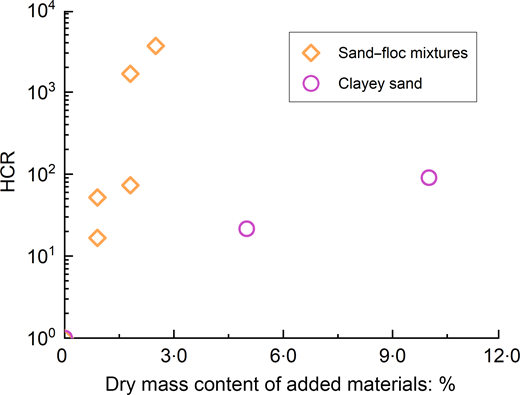
A number of falling head tests are performed to determine the relationship between the HCR and the dry mass contents of added materials. Clayey sand is fully compacted during preparation such that its hydraulic conductivity is measured around the densest state. Since the sand–floc mixtures are hard to compact due to their high water contents, their hydraulic conductivity is measured around the loosest state. Fig. 2 shows the results. Sand–floc mixtures have a much lower hydraulic conductivity than the pure sand. The magnitudes of the HCR of sand–floc mixtures range from 10 to 1000. Clayey sand can achieve an HCR of 10 to 100. Note that HCR equals 1 for pure sand. Lower Al–OM floc contents can achieve larger HCR than clay as Al–OM precipitates occur as floc-like structures, which are larger than clay particles. This implies that the flocs have a higher potential to block the (larger) pore throats of soils. The relationships of sand–floc mixtures and clayey sand agree well with the results from Kaptein (2021) and Revil & Cathles (1999), respectively. The dispersion of the data in Fig. 2 is caused by the heterogeneity of the materials.
Experimental set-up
BEP tests use the experimental set-up modified from the one for small-scale experiments described by Van Beek et al. (2015) and Rosenbrand et al. (2022b). Fig. 3 shows the experimental set-up in this research. The rectangular box containing the testing sample has transparent acrylate plates at the top and the bottom as well as the front and the back. The inner dimensions of the box are 525 × 300 mm × 100 mm (length × height × width). The silicone gel applied on the bottom side of the cover plate ensures good contacts between the sample and the cover. The box has measurement holes connected to piezometers on the top, front and bottom plates. The inlet filter adjacent to the inlet can distribute the inflow of water. The outlet hole on the top plate allows outflow of water, and the outlet cylinder over the outlet hole enables the deposition of eroded materials. The height (or thickness) of the hole has been kept as small as possible to prevent large head losses in the exit that would influence the global gradient. Outside the box, a set of hydraulic hoses supply water to the box and collect the outflow. The water level at the upstream side is maintained constant throughout the test, while the downstream head can be lowered stepwise. The maximum head drop of the set-up is 1·2 m. The scale can continuously record the weight of the outflow during the tests. A camera over the box captures the experimental phenomena of the pipe and the barrier.
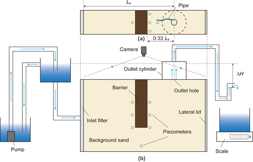
Scheme of the experimental set-up of BEP tests: (a) plan (top) view and (b) front view. Ls is the distance from the inlet to the outlet
Scheme of the experimental set-up of BEP tests: (a) plan (top) view and (b) front view. Ls is the distance from the inlet to the outlet
Testing procedures
Prior to the start of testing, the samples are prepared in the box by rotating it to a position with the inlet facing the floor and removing the lateral lid at the downstream side. In this way, the samples are built up from the inlet filter to the lateral lid. This sample preparation method is similar to that used in small-scale experiments by Van Beek et al. (2015) and Rosenbrand et al. (2022b). At first, dry sand is continuously rained into de-aired water and simultaneously tamped to obtain a saturated and homogeneous sample.
Fabricating a barrier consists of a series of specific procedures. First, the sand–floc mixture or clayey sand is rained onto the underlying wet sand to create a thin layer (5–10 mm thick) of the barrier. Second, water is sprayed onto the thin layer. Third, the thin layer is carefully tamped to achieve both compaction and saturation with the sprayed water. These three procedures are repeated to fabricate a barrier layer by layer until the thickness (width) of the barrier reaches the desired level. The key is to place the barrier materials layer by layer and saturate each layer by spraying water and tamping. This avoids particle segregation when the barrier materials are directly rained into water.
Lastly, the remaining space of the box is filled with dry sand using the same method as mentioned earlier. The resulting relative density of the background sand as a whole by this method is listed later in Table 3 for all samples. When sample preparation finishes, the lateral lid is closed, and the box resumes the normal position for testing. The relative densities of the background sand are lower in test S4 and C3 than in the other tests. This may be related to sub-optimal compaction of the sand near the downstream boundary of the barrier. In addition, the tests start after 2–15 hours following sample preparation.
At the beginning of the tests, the hydraulic hoses and the outlet cylinder are filled with water. Lowering the outlet hydraulic hose can apply a total hydraulic head drop across the sample indicated in Fig. 3(a). In general, the total hydraulic head drop is increased step by step with 1 cm every 5 min, at which the critical values of the total hydraulic gradient could be determined during the test. If piping occurs, the total hydraulic head drop is maintained until the pipe progression reaches equilibrium, and for a minimum of 5 min. A short waiting time after reaching stable conditions is common for BEP experiments (Rosenbrand et al., 2022b; Van Beek et al., 2015). Five minutes are considered sufficient, as the sand is fully saturated and the water pressures in the sand respond quickly to the hydraulic head increment, and the onset of particle movement is also generally immediately observed after head increment. Vandenboer et al. (2019) demonstrated that a step-wise increase of the hydraulic head results in pipe progression that is similar to a gradual head increase. It is noted that erosion of particles within the matrix (suffusion or suffosion) can cause gradual changes in the flow velocity in the pores, resulting in an effect of the loading path. This is observed by Luo et al. (2013) and Rochim et al. (2017), but is likely not to be applicable to BEP experiments with uniform sands. The tests end either when a pipe reaches the inlet filter or when the maximum head drop is reached. During the test, images of samples, local hydraulic heads and mass of outflow are recorded at a frequency of 0·1 Hz.
Overview of experiments
The experimental programme, listed in Table 2, is aimed at investigating whether low-permeability barriers can mitigate BEP and what influences the mitigating effect. Three series of small-scale experiments are performed using the experimental set-up in Fig. 3. They are reference tests with no barrier, the sand–floc barrier tests and the clayey barriers tests. The reference tests can provide evidence of pipe progression and critical gradients in pure B15 sand, which can be compared with barrier tests. The clayey barrier tests serve as benchmarks to verify whether the sand–floc barriers can act as low-permeability barriers. To study the impact factors of barriers on mitigation of piping, barrier depths and the fine mass contents of barriers are changed. The floc and clay contents are selected based on the results of permeability tests in Fig. 2. The intention is to create barriers with HCR of 25 and 100. Therefore, a content of 1% flocs or 5% clay is selected for HCR = 25, and 1·5% flocs or 10% clay is selected for HCR = 100.
Overview of backward erosion piping (BEP) tests
| Test series | Test label | Barrier depth: m | Depth ratio | Barrier material |
|---|---|---|---|---|
| No barrier | R1 | — | — | — |
| R2 | — | — | — | |
| Sand–floc barrier | S1 | 15 | 1/2 | 1·5% Al–OM flocs/98·5% sand |
| S2 | 15 | 1/2 | 1·5% Al–OM flocs/98·5% sand | |
| S3 | 20 | 2/3 | 1% Al–OM flocs/99% sand | |
| S4 | 20 | 2/3 | 1% Al–OM flocs/99% sand | |
| S5 | 20 | 2/3 | 1·5% Al–OM flocs/98·5% sand | |
| S6 | 20 | 2/3 | 1·5% Al–OM flocs/98·5% sand | |
| Clayey barrier | C1 | 15 | 1/2 | 10% clay/90% sand |
| C2 | 15 | 1/2 | 10% clay/90% sand | |
| C3 | 20 | 2/3 | 5% clay/95% sand | |
| C4 | 20 | 2/3 | 5% clay/95% sand | |
| C5 | 20 | 2/3 | 10% clay/90% sand | |
| C6 | 20 | 2/3 | 10% clay/90% sand |
This research does not investigate the influence of the distance between the flow outlet and the barrier in the experimental programme. In designing mitigation measures against pipe progression (not initiation – note that the existence of the flow outlet is a prerequisite of BEP), it is common to assume the locations of sand boils are known in advance. This is possible as sand boils are often observed in flood defence systems when the water level rises. When sand boils are not observed, the weakest spot is selected based on subsurface data, hydraulic conditions and the geometry of the surface. Due to the constraint of the experimental set-up, the influence of various problem geometries can be more conveniently investigated through numerical modelling.
Data analyses
Estimating the HCR of barriers is a prerequisite for analyses of their impact on the processes of BEP. The hydraulic conductivity of the barriers in the tests is uncertain due to the heterogeneity of the barriers originating from sample preparation, although the dry mass content of the added materials to fabricate barriers is known (Table 2). Therefore, a primary task of data analyses consists in inferring the HCR of testing barriers from measurement data.
This research uses a back-calculation scheme to infer the HCR of barriers from the measurements of local hydraulic heads. A two-dimensional finite-element model is built in COMSOL Multiphysics 5·6 (COMSOL, 2020) to simulate the hydraulic heads at measurement points in barrier tests without consideration of piping. The Appendix introduces the details of the numerical model. The principle of the back-calculation scheme lies in matching the hydraulic heads at the same locations between simulating and experimental results. This can be achieved by varying the values of the barrier HCR in the model until a best-matched HCR is found. The hydraulic heads used for the back-calculation are selected from measurements at the initial stage of tests when there is no pipe or only a small pipe, to minimise the effect of piping on hydraulic conductivity estimation.
The hydraulic conductivity of the sand is known a priori based on its porosity measured in the tests. As Table 1 provides the limits of porosity and hydraulic conductivity, a linear relationship is assumed as
where Ksand is the saturated hydraulic conductivity of sand and nsand is the porosity of sand.
In order to find the HCR that leads to the best match, the mean absolute error (MAE) function is constructed as
and
where η is the ratio of the local hydraulic head (hi) to the total hydraulic head drop (ΔH); M is the total number of piezometers used in the calculation of MAE; N is the total number of steps used in calculation of the averaged local hydraulic heads in experiments. In fact, experimental results of hydraulic heads may be unstable due to clogging of piezometers or the inevitable effect of piping. Therefore, the values of M and N vary among tests to find the most stable results for the back-calculation.
RESULTS AND DISCUSSION
This section presents and discusses the experimental results, including observations of the piping process, flow rates and total hydraulic gradients. It contributes to characterisation of the general behaviour of BEP in the presence of low-permeability barriers.
Results of the reference tests
In the reference tests, barriers do not exist. Applying a small total hydraulic gradient can cause sand boiling within the outlet hole. At a higher total hydraulic gradient, more sand is carried out to the outlet hole by the water flow, and consequently, this erosion process forms a pipe near the outlet hole. As the total hydraulic gradient increases, the pipe progresses towards the upstream inlet. Equilibrium states are observed in test R1, in which the pipe stops progressing until the total hydraulic gradient increases further. In test R2, the pipe forms and progresses to the inlet without reaching an equilibrium.
Figure 4 shows the outflow Darcy velocity and normalised pipe lengths of the reference tests. The outflow Darcy velocity can normalise the effect of the outlet size studied by Miesel (1978), and it is closely related to the pipe initiation (Richards & Reddy, 2012). The outflow Darcy velocity is computed by
where Q is the measured flow rates by the scale (g/s); ρ is the density of water equal to 1 g/cm3; Aout is the cross-sectional area of the outlet. The normalised pipe length l∗ is calculated as the ratio of the measured pipe length to the seepage length. As proposed by Vandenboer et al. (2018), the pipe length is computed as the length of the pipe projected on the longitudinal direction of the experimental set-up (the actual meandering pipe length is often somewhat longer). The total hydraulic gradient is calculated by dividing the total head drop by the seepage length.
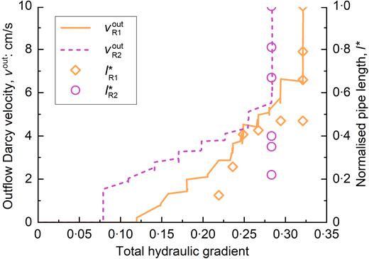
The pipes in tests R1 and R2 reach the inlet at total hydraulic gradients of 0·32 and 0·28, respectively, followed by surges of flow in Fig. 4. The average of these two gradients is termed the reference critical gradient, at which piping failures occur in pure sand samples. The observations of the piping process agree with those in other BEP tests with pure sands (Van Beek, 2015; Van Beek et al., 2015).
Figure 5(a) shows the pipe when it reaches the inlet. Until the end of the reference tests, all sand particles flowing out deposit around the outlet hole. This is also observed in all barrier tests.
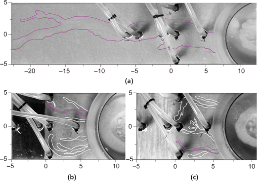
Top views of pipes in BEP tests when the pipes are fully developed: (a) reference test R2, Gtotal = 0·28; (b) sand–floc barrier test S5, Gtotal = 3·00; and (c) clayey barrier test C6, Gtotal = 2·38. The line contours delineate the pipes. In (b) and (c), the purple represents the first branch reaching the barrier, and the white represents others. The origin of the horizontal axis is chosen at the downstream boundary of the barrier (unit: cm)
Top views of pipes in BEP tests when the pipes are fully developed: (a) reference test R2, Gtotal = 0·28; (b) sand–floc barrier test S5, Gtotal = 3·00; and (c) clayey barrier test C6, Gtotal = 2·38. The line contours delineate the pipes. In (b) and (c), the purple represents the first branch reaching the barrier, and the white represents others. The origin of the horizontal axis is chosen at the downstream boundary of the barrier (unit: cm)
Results of the barrier tests
Pipe progression in barrier tests is significantly different from that in the reference tests. The observed stages of progression during barrier tests are defined as pipe progression, barrier interception, pipe branching and piping failure, displayed in Fig. 6.
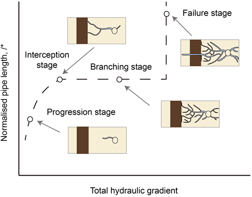
Piping is initiated in all barrier tests in this work. A low-permeability barrier cannot entirely prevent pipe initiation. However, the barrier makes it much harder for the pipe to progress. Table 3 registers more details about the required total hydraulic gradients for pipe progression. For example, the required total hydraulic gradient for the pipe to reach l∗ of 0·2 is 0·5 to 1·2 times higher in barrier tests than in reference tests. When the pipe approaches the barrier, its progression is even more impeded by the barrier. This is indicated in Fig. 7 by the decreasing slope of the trends of the normalised pipe length. In tests S1, C2 and C4, the normalised pipe length even arrives at a temporary plateau before the pipe reaches the barrier. In addition to the length, the widths of pipes in barrier tests in Figs 5(b) and 5(c) are smaller than those in the reference test in Fig. 5(a). This stage, in which a fine pipe progresses towards the barrier with increments of the total hydraulic gradient, is termed the progression stage in Fig. 6.
Experimental results of BEP tests
| Test | Dr,sand: % | Ksand: ×10−5 m/s | Gtotal at l* = 0·2 | Gtotal at interception | Gtotal at failure | HCR of barriers |
|---|---|---|---|---|---|---|
| R1 | 83·9 | 6·56 | 0·23 | Not applicable | 0·32 | Not applicable |
| R2 | 92·8 | 6·03 | 0·28 | Not applicable | 0·28 | Not applicable |
| S1 | 106·4 | 5·23 | 0·40 | 2·23 | 2·51 | 90 |
| S2 | 92·8 | 6·02 | 0·47 | 1·96 | Not applicable | 100 |
| S3 | 94·9 | 5·91 | 0·46 | 1·65 | 3·03 | 40 |
| S4 | 54·3 | 8·30 | 0·37 | 1·63 | Not applicable | 100 |
| S5 | 90·7 | 6·16 | 0·43 | 1·38 | 3·10 | 100 |
| S6 | 93·8 | 5·97 | 0·41 | 1·69 | Not applicable | 100 |
| C1 | 94·6 | 5·93 | 0·37 | 0·67 | 1·82 | 20 |
| C2 | 89·1 | 6·25 | 0·38 | 1·33 | Not applicable | 30 |
| C3 | 68·6 | 7·46 | 0·42 | 0·60 | 0·83 | 7 |
| C4 | 94·4 | 5·94 | 0·37 | 0·99 | 1·15 | 7 |
| C5 | 93·8 | 5·97 | 0·53 | 1·77 | Not applicable | 70 |
| C6 | 102·6 | 5·45 | 0·57 | 1·36 | Not applicable | 20 |
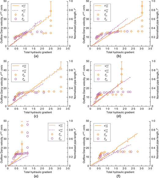
Outflow Darcy velocity and normalised pipe lengths of the barrier tests: (a) S1 and S2; (b) S3 and S4; (c) S5 and S6; (d) C1 and C2; (e) C3 and C4; (f) C5 and C6
Outflow Darcy velocity and normalised pipe lengths of the barrier tests: (a) S1 and S2; (b) S3 and S4; (c) S5 and S6; (d) C1 and C2; (e) C3 and C4; (f) C5 and C6
Once the pipe reaches the barrier, the pipe length completely stops increasing in Fig. 7. This means the barrier intercepts the pipe. This marks the interception stage in Fig. 6, and the corresponding total hydraulic gradients are identified as interception gradients in this research, listed in Table 3. During this stage, no erosion of barrier materials is immediately observed. Instead, the pipe is continuously eroded in depth and width when the total hydraulic gradient increases. The pipe may progress laterally along the downstream boundary of the barrier.
When an additional pipe branch forms, the branching stage begins. Pipe branching is universally observed in barrier tests, as shown in Figs 5(b) and 5(c). This is due to the fact that the resistance of sand against erosion is spatially varying and that pipe progression tends to follow the path of weakest resistance against erosion (Robbins & Griffiths, 2021; Robbins et al., 2021). Increases of the total hydraulic gradient after the pipe reaches the barrier can activate more weak paths for pipe progression and, consequently, increase branches of pipes. The branching stage is a transition from the interception stage to the failure stage shown in Fig. 6.
At the failure stage in Fig. 6, the barrier can fail at a constant total hydraulic gradient. This hydraulic gradient is identified as the failure gradient in the current research, listed in Table 3. Barrier failures are initiated by fusion of pipe branches. Several pipe branches merge and form larger eroded channels or even an eroded plane. This means that soil erosion is no longer restricted in individual pipes of small sizes but takes place in an extensive zone instead. As this intense erosion propagates, the sand near the downstream side of the barrier is weakened so that water can gradually erode the barrier from its downstream boundary. The erosion of the barrier is a suffusion process, starting with erosion and transport of the finest fraction. While the barrier keeps losing its finest components, its resistance to BEP decreases. This results in the formation of a piping channel inside the barrier. Eventually, the pipe penetrates through the barrier and progresses to the inlet (l∗ increases to 1) after the plateau in Figs 7(a)–7(e). This fully developed pipe allows a huge amount of water to flow, indicated by the surges of outflow velocity. Since the failure of the barriers develops over time at constant total hydraulic gradients, the resistance of barriers is time-dependent at the failure stage.
The experimental results demonstrate that both types of barriers can achieve a significant reduction in hydraulic conductivity compared with the background sand, ranging from seven to 100 times. In addition, both types of barriers can largely mitigate BEP. Therefore, it is considered that the sand–floc barriers produced in the tests can effectively function as low-permeability barriers, similar to the clayey barriers.
Functions of low-permeability barriers in mitigating piping
To account for the mitigating mechanisms, two functions of barriers are essential. Understanding these functions is important to the design of barriers.
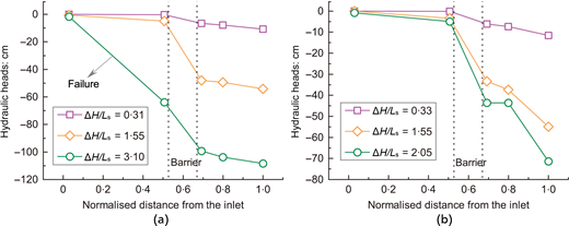
One function of low-permeability barriers is the ability to hinder pipe progression before interception. The reason behind this function is that barriers can significantly dissipate the hydraulic head at the soil–cover interface due to two mechanisms. First, the barrier consumes a large amount of the energy of water permeating through it. Second, the long seepage length causes considerable energy loss for water circumventing the barrier. Normalised heads measured at the soil–cover interface in Fig. 8 reveal the impact of barriers at the progression stage. The hydraulic head decreases more across the barrier domain in the barrier test than in the reference test, leaving less downstream hydraulic gradient to propel pipe progression.
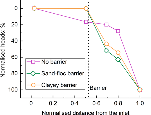
Normalised heads at the soil–cover interface at the total hydraulic gradient of 0·21 in tests R1, S5 and C6
Normalised heads at the soil–cover interface at the total hydraulic gradient of 0·21 in tests R1, S5 and C6
This function is particularly important when a perfectly homogeneous barrier is hard to achieve in practice or when the barrier has low erosion resistance. The mitigating effect is quantified by the interception gradients given in Table 3. They are all much greater than the reference critical gradient, ranging from 2·2 to 7·4 times the latter. Although the interception gradient may be subject to scale and geometric effects, the results imply that the design of barriers could use the interception gradient as an objective to achieve a certain level of mitigating effect. This would require simulation of the pipe formation process near the barrier at different scales. This design perspective is fundamentally different from those focusing on the critical gradient in the design of a barrier (Achmus & Mansour, 2006; Zhou et al., 2007; Okajima & Tanaka, 2008; Zhou et al., 2012).
Another function of low-permeability barriers is related to the ability to remain intact under a large hydraulic gradient. At the interception stage and the branching stage, increasing the total hydraulic gradient still causes erosion of the sand by secondary erosion or branching, but not erosion of barrier materials. Both types of barriers can sustain a large hydraulic head drop across them, shown by the lines of ΔH/Ls equal to 1·55 in Fig. 9. Such high resistance against erosion is due to clogging induced by fine grains (Jäger et al., 2017; Wautier et al., 2019). In addition, the barrier can reduce the fluidisation of the sand near its downstream boundary, thereby mitigating the formation of vertical pipes. This could be due to the horizontal flow through the barrier and relatively large depth ratios of barriers in the tests. In shorter and impermeable barrier tests (Achmus & Mansour, 2006; Zhou et al., 2007; Okajima & Tanaka, 2008), it is frequently observed that the pipe progresses vertically along the barrier and eventually circumvents it.
Only if the total hydraulic gradient reaches the failure gradient can the local hydraulic force from the flow exceed the threshold needed to induce grain detachment within the barrier and, consequently, cause its failure. In this work, the measured failure gradients are approximately 1·13 to 2·72 times the interception gradients, derived from the values in Table 3. These findings indicate that the function of barriers acting after interception offers additional safety margin to the barrier when designed by the interception gradient.
Impact of the hydraulic conductivity reduction
The findings of tests suggest the impact of the HCR of barriers on pipe progression and barrier failures. For barriers at a depth ratio of 2/3 in Fig. 10(a), higher HCR results in a larger interception gradient when HCR is not higher than 40, but increasing HCR beyond 40 times does not lead to additional enhancement in interception gradients. A similar trend is also observed in Fig. 10(b) for the failure gradients of barriers. At a depth ratio of 2/3, the failure gradient at HCR of 40 is close to that at HCR of 100, but is significantly larger than those at HCR of 7.
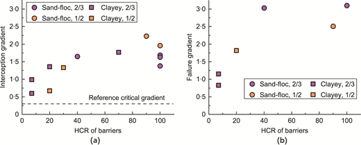
Critical values of total hydraulic gradients: (a) at pipe interception and (b) at failure of barriers
Critical values of total hydraulic gradients: (a) at pipe interception and (b) at failure of barriers
The essential mechanism behind the impact of the HCR of barriers is associated with the energy dissipation of water mentioned previously. When the HCR is small, its increase causes more energy dissipation of water that permeates through the barriers. This decreases the residual energy of water at the downstream side to drive pipe progression. When the HCR is sufficiently large, water predominantly tends to bypass the barrier rather than permeate through it. Since the flow through the barrier is exceedingly small, increasing the HCR barely results in greater energy dissipation of water. Under such circumstances, the barrier behaves as nearly impermeable.
Impact of the barrier depth ratio
The barrier depth ratio determines the seepage length circumventing the barrier. Therefore, varying the barrier depth ratio can affect pipe progression. Both interception and failure gradients should increase with the increment of the barrier depth ratio, because a longer barrier depth renders a longer seepage length circumventing the barrier, inducing greater energy dissipation of water.
In Fig. 10(a), when the HCR is relatively small, a larger barrier depth ratio leads to a larger interception gradient. Similarly, the failure gradient increases with the barrier depth ratio in Fig. 10(b). These experimental results agree with the aforementioned hypothesis.
However, some results contradict this hypothesis. When the HCR is relatively large in Fig. 10(a), the barriers at a depth ratio of 2/3 result in smaller interception gradients. This could be explained by the concentration of flow lines near the pipe tip when the pipe approaches the barrier. For a deeper and less permeable barrier, the flow lines appear to be more vertical and concentrated near its downstream boundary due to less horizontal flow through the barrier. These denser flow lines can lead to a larger flow velocity, which promotes stronger pipe progression.
The impact of the barrier depth ratio on pipe progression may depend on the HCR. Note that the number of tests on the barrier depth ratio is limited.
Barrier heterogeneity and challenges of sample preparation
Although the processes of sample preparation are aimed at achieving a homogeneous barrier, subsequent visual inspection of samples after preparation reveals that all barriers are heterogeneous. Furthermore, the heterogeneity pattern of the two types of barriers is different. Sand–floc barriers typically possess a patchy pattern of heterogeneity, as illustrated in Fig. 11(a). There are patches of sand–floc mixtures with low floc contents randomly distributed within the barrier. Moreover, sand intrudes into the downstream boundary of the sand–floc barrier, forming an irregular shape of the boundary. Differently from sand–floc barriers, clayey barriers exhibit a layered pattern of heterogeneity. Clayey sand layers with different clay contents exist within the barrier in Fig. 11(b). The boundaries of the clayey barrier are mostly regular.
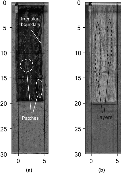
Images of heterogeneity of barriers: (a) the sand–floc barrier; (b) the clayey barrier (unit: cm)
Images of heterogeneity of barriers: (a) the sand–floc barrier; (b) the clayey barrier (unit: cm)
This difference of the heterogeneity pattern stems from different methods of sample preparation for the two types of barriers. When creating sand–floc barriers, the mixtures incorporate water through the floc solution. The water content of the sand–floc mixtures ranges from 17 to 29% during sample preparation. This pore water has the potential to generate excess pore water pressure and trigger particle segregation during compaction, thereby hindering the compaction process of the mixtures. Owing to their lack of compaction, the sand–floc barriers are soft and prone to sand intrusion at the downstream boundary. Therefore, sand–floc barriers show the patchy pattern of heterogeneity and an irregular upstream boundary. Unlike sand–floc mixtures, the clayey sand has relatively low water contents, allowing a gradual layer-by-layer compaction process. This compaction process eventually leads to the layered pattern of heterogeneity of clayey barriers.
Distinct levels of compaction between the two types of barriers cause notable difference in their porosity of the sand skeleton. Because of insufficient compaction, the porosity of sand in sand–floc barriers is close to the value of the loosest pure sand. Clayey barriers experience adequate compaction during preparation. Therefore, their porosity of sand is close to the value of the densest pure sand.
The barrier heterogeneity brings uncertainty to the tests and their results, particularly in the tests of sand–floc barriers. The intrusion of sand into the upstream boundary reduces the width of the barrier and loosens the sand nearby. These local variations near the barrier boundary could have an impact on the pipe when it approaches the barrier. In addition, patches of low floc contents could lead to the formation of preferential flow paths that allow concentration of flow and initiate internal erosion of barriers.
It is worth noting that the sand–floc barrier made by mixing in the laboratory cannot fully represent that created by injection of Al–OM flocs in the field. Injection of flocs to soils generates a microstructure, in which the flocs precipitated under low-shear conditions clog the pore throats (Zhou et al., 2022). The injection-made barrier could be more heterogeneous in terms of the floc content due to spatially varying permeability of in situ soils. In the laboratory, it is difficult for mixing to reproduce the microstructure and the heterogeneity of the injection-made barrier. Nonetheless, the HCR and the depth of the barrier are relatively easy to control by the mixing–placing method. Therefore, this method is used in sample preparation in the present research to better capture the effects of the HCR and the depth, which are two important parameters in the design of a barrier.
CONCLUSIONS
This paper investigates the potential of a novel engineering solution to mitigate BEP, in which a low-permeability barrier is created by injecting Al–OM flocs within soils susceptible to internal erosion. A series of laboratory tests is conducted to observe the behaviour of pipes in the presence of barriers and gain insights into the mitigating mechanisms. In addition to the sand–floc barriers, clayey barriers are also tested. The results of the barrier tests are compared with those of the reference tests, in which no barrier is present.
The experimental findings demonstrate that the sand–floc barriers behave as low-permeability barriers similar to the clayey barriers and show substantial capability in the mitigation of BEP. The barrier tests exhibit four stages in general: a progression stage, an interception stage, a branching stage and a failure stage. During the progression stage, a larger total hydraulic gradient is required for the pipe to reach a certain length in the presence of a barrier compared the reference tests. Upon reaching the barrier, the pipe is intercepted, and the barrier resists internal erosion. This resistance persists until a sufficiently high hydraulic gradient is applied, at which point the pipe penetrates the barrier, leading to failure. The interception gradients are 2·2–7·4 times the reference critical gradient, while the failure gradients range from 2·8 to 10·3 times the reference critical gradient.
Based on the experimental results, this paper has analysed and discussed how the low-permeability barriers mitigate BEP. It is found that barriers can significantly dissipate the hydraulic head and reduce the local hydraulic gradient near the pipe tip. This mitigating effect can be quantified by the interception gradients. Furthermore, barriers can resist internal erosion by clogging and prevent fluidisation of sand after interception, which can be evaluated by the failure gradients.
The HCR and the depth ratio of barriers influence the mitigating effects. When the HCR is relatively low, raising the HCR of barriers can significantly improve the interception and failure gradients, that is, the mitigating effects on BEP. Such an improvement is not obvious when the HCR exceeds a threshold, typically around 40. The impact of the barrier depth ratio may be dependent on the HCR, which is uncertain due to a limited number of tests.
The barrier heterogeneity gives rise to scattering of results. The heterogeneity patterns are different for the two types of barriers. The sand–floc barriers have a patchy pattern, while the clayey barriers show a layered pattern. The difference of heterogeneity patterns is associated with different degrees of compaction during sample preparation.
The findings of this research highlight the effectiveness of low-permeability barriers created by Al–OM flocs in mitigating BEP. The experimental results demonstrate the concept of using the interception gradient as a design objective of low-permeability barriers rather than the failure gradient. For prospective work, attention should be paid to the effect of the scale and the geometric properties. Large-scale tests need to be performed with barriers created by injection of Al–OM flocs to corroborate their potential in the field. Further numerical studies, validated by the results of this research, are required to explore the effect of barrier heterogeneity, the scale and the configuration on mitigation of piping.
ACKNOWLEDGEMENT
This research was funded by the water authority Hoogheemraadschap de Stichtse Rijnlanden through the Dutch Flood Protection Programme.
REFERENCES
APPENDIX. NUMERICAL MODEL FOR DATA ANALYSES
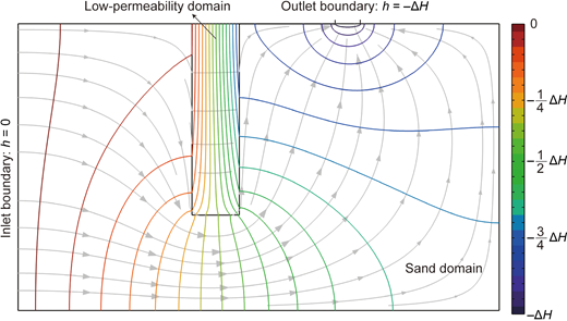
The numerical model (Fig. 12) utilises the Subsurface Flow Module (COMSOL, 2020) to simulate two-dimensional (2D) water flow in the experimental box. The model assumes that no pipe is developed in the sample, and therefore, the material parameters can remain constant in the simulation. The reason behind the 2D assumption is that the width of the experimental box is relatively small compared to its length and height. The boundary conditions are defined by a constant hydraulic head of zero at the inlet and a varying hydraulic head of −ΔH at the outlet, while a no-flow condition is set at other boundaries of the box. The low-permeability domain and the sand domain, defined by different parameters of permeability, represent the barrier and the sand in the test. The depth of the low-permeability domain is adjustable in order to meet the actual barrier depth. The hydraulic conductivity of the sand domain in the model refers to the results of Ksand in Table 3. In data analyses, the hydraulic conductivity of the low-permeability domain is varied to search the best-fit hydraulic conductivity against the experimental results.
Discussion on this paper closes 1 May 2026; for further details see p. ii.

