Slope movements are generally classified into four different phases: pre-failure, failure, post-failure and eventual reactivation. In engineering applications, the pre-failure and failure phases are usually analysed using traditional numerical techniques, such as the finite-element method and the finite-difference method. However, these methods are often based on the assumption of small deformations and consequently are unsuitable for analysing the slope behaviour during the post-failure stage, which is usually characterised by very large deformations. To overcome this shortcoming, the material point method (MPM) is employed in the present study. Specifically, MPM is used to perform an analysis of a landslide in sensitive clays that occurred at Saint-Jude (Quebec, Canada) in 2010. To assess the accuracy of the analysis, the final profile and the displacement magnitude detected after the event are compared with those obtained by the numerical simulation. The results provided by MPM are in satisfactory agreement with field observations. The failure mechanism and the development of the failure surface within the slope are also reproduced successfully. These results also show that MPM is an attractive method for analysing the kinematics of landslides in sensitive clays, requiring also a limited number of conventional geotechnical parameters as input data.
Notation
- C
Courant number
- cu
undrained shear strength
- cuo
undisturbed undrained shear strength
- cur
remoulded undrained shear strength
- E′
effective Young’s modulus of the soil
- Eb
Young’s modulus of the building material
- Eu
undrained Young’s modulus of the soil
deviatoric part of the plastic strain tensor
- IL
index of liquidity
- t
time
- α
coefficient of local damping
- γ
unit weight of the soil
- γb
unit weight of the building material
- Δtcr
critical time step
deviatoric plastic strain invariant
- λ
model parameter controlling the strength reduction rate
- υ′
Poisson’s ratio of the soil
- υb
Poisson’s ratio of the building material
- φ′
angle of shearing resistance
- ψ
dilatancy angle
Introduction
Slope movements and failure mechanisms are generally schematised into four different stages (Leroueil, 2001): pre-failure stage, including all deformation processes that occur in the slope before failure; failure stage, when a continuous shear surface forms within the slope; post-failure stage, in which the unstable soil mass moves at a high displacement rate followed by a progressive decrease in the velocity until motion stops; and reactivation stage, with the landslide body periodically moving along one or several pre-existing shear surfaces. Nevertheless, slope stability is commonly dealt with by accounting for the deformation processes occurring only in the pre-failure and failure stages by using simplified methods (Conte and Troncone, 2011, 2012a, 2012b, 2018; Conte et al., 2017, 2022; Duncan, 1996; Gottardi and Butterfield, 2001; Troncone et al., 2021) and traditional numerical techniques (e.g. the finite-element method (FEM)) referring to a Lagrangian approach, under the assumptions of small deformations (Conte et al., 2018; Griffiths and Lane, 1999; Potts et al., 1990; Troncone, 2005; Troncone et al., 2014). In the latter methods, the continuum medium is schematised by a computational mesh that deforms with it, leading to numerical drawbacks when the elements attain high levels of distortion, as usually occurs after the development of a slip surface. Therefore, such an approach is in principle unable to deal with the post-failure stage of landslides when large deformations occur. Recently, more advanced numerical methods have been proposed to deal with problems involving large deformations, incorporating the advantages of both Lagrangian and Eulerian approaches. The methods available in the literature for dealing with large-deformation problems can be categorised into two distinct approaches: the discrete approach and the continuum one (Scaringi et al., 2018). The distinct-element method (Calvetti et al., 2017) and the particle flow code (Li et al., 2021) are included in the former category. Among the most used continuum approaches for modelling landslide problems are the smoothed particle hydrodynamics method (Bui et al., 2011; Dai et al., 2014; Pastor et al., 2009; Pirulli and Pastor, 2012), the Eulerian-based large-deformation FEM (Wang et al., 2021) and the material point method (MPM) (Abe and Konagai, 2016; Alonso et al., 2015; Bandara and Soga, 2015; Bhandari et al., 2016; Ceccato et al., 2020; Fern et al., 2019; Li et al., 2016; Liang et al., 2020; Nakajima et al., 2019; Nguyen et al., 2022; Rohe and Martinelli, 2017; Soga et al., 2016; Sołowski and Sloan, 2015; Troncone et al., 2022a; Yerro et al., 2016; Zabala and Alonso, 2011).
Soga et al. (2016) provided a comprehensive review of these methods, highlighting the efficiency of MPM in analysing the deformation processes of landslides, including the post-failure stage. Specifically, the main reasons for which MPM should be preferred to other methods are as follows: (a) it can be employed for the analysis of problems involving large deformations, because MPM is based on a continuum-based description of motion through an Eulerian–Lagrangian approach; (b) the implementation of MPM is similar to that of FEM, and advanced history-dependent constitutive models can be included; and (c) complex boundary conditions can be readily dealt with.
Recent developments concerning MPM can be found in the papers by Ma et al. (2022a, 2022b). These authors account for the effects of heterogeneous soil properties and spatial variability of shear strength using random field theory and generalised interpolation MPM integrated in a Monte Carlo approach within a probabilistic framework. Additionally, the same authors employed MPM to study the effects of soil anisotropy and fabric orientation on the post-failure stage of landslides (Ma et al., 2022c).
In the present work, MPM is employed to analyse a landslide that occurred in 2010 at Saint-Jude (Quebec, Canada) involving mainly a formation of sensitive clays. These soils may undergo a considerable reduction in strength when subjected to remoulding (Skempton and Northey, 1952), as it occurs during the run-out process of landslides. As a consequence, landslides involving very sensitive clays (often called quick clays) are generally characterised by a very high velocity and a very long run-out distance (comparable with those experienced by lateral spreads due to a liquefaction). These landslides have captured the interest of the international geotechnical community since the pioneering works by Skempton and Northey (1952) and Bjerrum and Landva (1966), inspired by the impressive events that occurred in Norway. However, the unavailability of suitable methods of analysis is one of the main obstacles to the advancement of knowledge about the kinematics of these natural disasters. In fact, very few case studies are documented in the literature concerning the post-failure analysis and kinematic behaviour of landslides in sensitive clays. For such landslides, most of the available papers focused only on the failure stage, without paying attention to post-failure analysis and to the prediction of the run-out distance of the landslide masses. Run-out analysis is a key step in landslide risk assessment and mitigation design (McDougall, 2017). In this context, the main objective of the present paper is the analysis of the deformation process (including the post-failure stage and run-out distance) and the kinematic behaviour of the Saint-Jude landslide by using MPM along with a strain-softening soil model.
The Saint-Jude landslide was deeply investigated by Locat et al. (2017) who provided a comprehensive description of the event and a detailed geotechnical and morphological analysis of the debris with a reconstitution of its dislocation mechanism. Following these authors, the landslide was triggered by a combination of river erosion and high pore water pressures existing in the slope. Subsequently, Zhang et al. (2020), using the particle FEM, provided an interpretation of the Saint-Jude landslide in terms of a retrogressive rotational mechanism consisting of a succession of rotational slides delimitated by multiple failure surfaces (see figure 5 of the paper by Zhang et al. (2020)). This mechanism accounts for the presence of grabens and horsts, also mentioned in the paper by Locat et al. (2017), but does not completely match the reconstruction made by the latter authors. Indeed, Locat et al. (2017: p. 1373) (in the conclusions of their study) pointed out that after the slope failure, ‘the main movement of the debris was mostly translational along the failure surface, with little or no rotation. This indicates that the landslide did not occur as the result of a succession of rotational slides’. The analysis performed in the present study concerns the failure and post-failure stages of the Saint-Jude landslide in order to define its failure mechanism and complete the understanding of the deformation processes that occurred during these stages, as well as propose MPM as an effective and very useful numerical technique for analysing landslides involving very sensitive clays.
Material point method
Numerical analyses are generally dealt with by referring to Lagrangian and Eulerian approaches (Zhang et al., 2017). In Lagrangian methods, a computational mesh deforms with the material, and consequently, history-dependent constitutive models can be easily implemented and material interfaces can be readily tracked. However, when dealing with large-deformation problems, Lagrangian methods suffer from a high mesh distortion, which leads to inaccuracies in calculation. In contrast, the mesh is undeformed and the material flows through it in Eulerian methods. Consequently, no element distortion occurs when dealing with large deformations. However, special procedures are required to identify the material interfaces and history dependency. As a consequence, Eulerian approaches are much more expensive from a computational point of view than Lagrangian ones. In this context, MPM has been developed to take advantage of both Lagrangian and Eulerian approaches, avoiding their shortcomings.
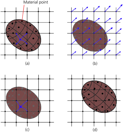
MPM was initially introduced by Sulsky et al. (1994) for modelling large deformations in the field of solid mechanics. In such an approach, the continuum medium is subdivided into subdomains, whose information (density, acceleration, velocity, displacement, mechanical characteristics, external loads and state variables) is concentrated within Lagrangian points, named material points. Movements of the material points define the motion of the soil. Furthermore, the material points are superimposed on a Eulerian mesh that is used to solve the governing equations, without carrying any permanent information. To allow the simulation of large displacements, the entire space in which material points are supposed to move during the whole simulation has to be covered by the Eulerian mesh. Briefly, the MPM calculation scheme is summed up in Figure 1.
Specifically, at the beginning of any calculation step, information contained in the material points is transferred to the nodes of the computational mesh, using common interpolation shape functions (Figure 1(a)). The governing equations are solved at the mesh nodes and the unknown variables are calculated, similarly to FEM (Figure 1(b)). Afterwards, the obtained information is used to update the acceleration, velocity and displacement of the material points and to calculate deformations and stresses (Figure 1(c)). Subsequently, material points’ positions are updated (Figure 1(d)), and the next calculation step is considered. Following this scheme, no permanent information is stored in the Eulerian mesh. In this way, large displacements are simulated while the mesh is kept undeformed during the entire simulation. Consequently, the accuracy of the calculation is ensured even when the material points are subjected to large displacements. In conclusion, the drawbacks of the Lagrangian and Eulerian approaches are overcome. Specifically, the computational effort is notably reduced in comparison with the Eulerian approach, as no special procedures are required to track material interfaces and to implement history-dependent constitutive models, and the problems related to mesh distortion (typical of Lagrangian approaches) are averted. Two main formulations are usually discerned in MPM (Fern et al., 2019): the single-point formulation and double-point one. Referring to the single-point formulation, the continuum medium is schematised by a single set of material points, representing both solid and fluid phases. In this context, the one-phase single-point formulation is suitable for modelling dry soils or saturated soils under drained or undrained conditions (Abe et al., 2017; Alonso et al., 2015; Conte et al., 2019, 2020; Troncone et al., 2022a, 2022b; Yerro et al., 2019). On the other hand, the two-phase single-point formulation can be used to model the behaviour of saturated soils under transient conditions (Giridharan et al., 2020; Nguyen et al., 2021; Troncone et al., 2019, 2020; Yerro et al., 2016), and the three-phase single-point formulation is employed for unsaturated soils (Yerro et al., 2015). Additionally, the behaviour of unsaturated soils can be also modelled by means of the two-phase single-point formulation with suction (Ceccato et al. 2021; Cuomo et al., 2021). These formulations are included in the code of the Anura3D (2023) software, which is employed to perform the analysis presented in the following section.
Analysis of the 2010 Saint-Jude landslide
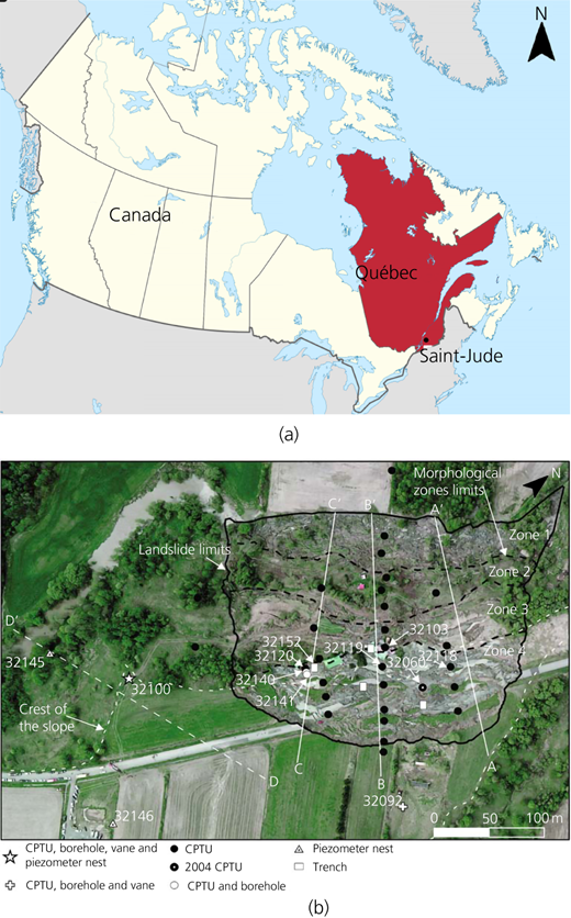
In this section, an analysis of the failure and post-failure stages of the landslide that occurred at Saint-Jude (Quebec, Canada) on 10 May 2010 is performed using MPM. A detailed description of this landslide is provided by Locat et al. (2017). Following these authors, the Saint-Jude landslide should have been triggered by natural causes. In particular, the erosion produced by the Salvail River, located at the base of the slope, along with the high pore water pressures observed in the slope were considered the main factors of triggering of the event. The landslide was characterised by a length of approximately 210 m and a width of about 270 m (Figure 2).
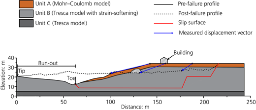
The maximum height of the head scarp was about 7 m. The contour of the landslide body was detected by Locat et al. (2017), as indicated in Figure 2. The subsoil of the Saint-Jude area is formed by three geological units denoted unit A, unit B and unit C (Figure 3). The shallowest one is unit A, which extends down to a depth of about 4 m from the slope surface and can be classified as a dense sand from a geotechnical point of view. Unit B, whose thickness is approximately 22 m, consists of a uniform sensitive clay with an overconsolidation ratio in the range 1.2–1.9. Finally, unit C is a stiff silty clay of low sensitivity with a thickness of approximately 5 m. The soil below these units is characterised by high shear strength, so that it can be considered the bedrock of the overlying soils. The available piezometric measurements showed that the groundwater level is very close to the ground surface (Locat et al., 2017).
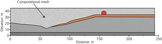
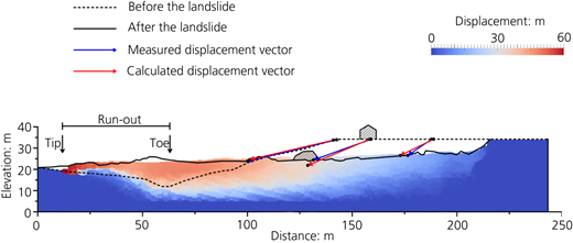
The landslide involved only unit A and unit B and presented the typical features of a spread in sensitive clays (Cruden and Varnes, 1996; Locat et al., 2011a). The failure surface was reconstructed by Locat et al. (2011b) on the basis of the results of many cone penetration tests. In particular, the profiles of the cone penetration tests performed in 2010, after the landslide, were compared with those obtained in 2004, before the landslide, which were used as a reference. Specifically, the base of the failure surface is determined as the depth where the profiles of the cone penetration tests obtained in 2010 change from a damaged state to the intact state measured in 2004. Most of this surface developed mainly just above the interface between unit B and unit C. Referring to section B–B′, whose trace is indicated in Figure 2, a representative geotechnical model of the slope is presented in Figure 3, where the location of the aforementioned failure surface is also indicated along with the slope profile detected before and after the landslide. This figure also shows the observed displacement vectors of some benchmark points located on the original ground surface. The run-out distance of the landslide body (i.e. the distance between the tip of the displaced soil and the toe of the failure surface) is about 60 m. Following Locat et al. (2017), at the beginning of 2010, the slope under consideration was precariously stable. These authors obtained a value of the slope safety factor equal to 1.03 using the limit equilibrium method (Morgenstern and Price, 1965). During the spring of the same year, a soil volume at the base of the slope was removed by river erosion that, in conjunction with the high pore water pressures existing in the slope, triggered the landslide. Unfortunately, the volume of the eroded soil is unknown. Nevertheless, following Locat et al. (2017), this volume should not have been very great considering that initially the slope was marginally stable. After the landslide triggering, the post-failure stage lasted a few minutes. Consequently, considering that the involved soil consists mainly of saturated clay, it is reasonable to assume that this process occurred under undrained conditions (Locat et al., 2017). In the following, the Saint-Jude landslide is analysed using the one-phase single-point formulation implemented in the MPM code Anura3D (2023). As this code employs an explicit dynamic formulation when solving the governing equations, the time step of calculation must be chosen to be less than a critical value to prevent numerical instability problems. The critical time step Δtcr is calculated according to the well-known Courant–Friedrichs–Lewy condition (Courant et al., 1967) as a function of the mesh size, elastic modulus and soil density. On the basis of the mesh size specified later, the elastic modulus indicated in Table 1 and a density of 1600 kg/m3, it turns out that a value of the time step equal to 0.1 s is sufficient to satisfy this condition. In addition, a Courant number C = 0.98 is used to correct this time step (Chmelnizkij and Grabe, 2019). The analysis is performed under the reasonable assumption of plane-strain conditions. For this purpose, a computational mesh made up of triangular elements with an average element size of 1.5 m is employed. This value was chosen to perform an accurate analysis while avoiding extremely high computational efforts. This mesh is shown in Figure 4 and refers to the longitudinal section of trace B–B′ located in the central part of the landslide body (Figure 2).
Three material points are initially distributed for each active element. Boundary conditions are simulated by hinges at the bottom of the model so that both vertical and horizontal displacements are prevented at this side, whereas rollers are employed on the vertical edges to prevent displacements in the horizontal direction. No failure surface is preventively imposed. Following Locat et al. (2017), in view of the evidence that the landslide lasted only a few minutes, the analysis is performed under undrained conditions for the clayey soils (unit B and unit C) with the soil parameters specified in Table 1. In contrast, fully drained conditions are assumed for unit A, consisting of a sandy soil, whose parameters are also shown in Table 1. For the sake of completeness, the presence of the building shown in Figure 3 is also accounted for in the simulation. This is also used as a benchmark to compare the displacements calculated by using MPM with the measured ones. The building is represented in an approximate manner by an elastic cluster with a value of the unit weight, γb = 12 kN/m3. To avoid numerical issues due to the marked difference in the stiffness of the involved materials, the Young’s modulus and Poisson’s ratio of this cluster are assumed Eb = 50 000 kPa and υb = 0.2, respectively.
The well-known procedure of gravity loading was used to generate the initial stress state of the slope. As this slope was marginally stable before the occurrence of the event (Locat et al., 2017), the gravity loading was generated under the assumption that all materials would behave elastically to avoid any failure in this stage. A similar approach was also employed for successfully simulating other landslides documented in the literature (Conte et al., 2019; Yerro et al., 2019). Referring to unit B, which was the formation mainly involved in the landslide body, typical values of Young’s modulus and Poisson’s ratio referring to drained conditions were E′ = 21 MPa and υ′ = 0.25, respectively (Locat et al., 2013). Since the analysis of the Saint-Jude landslide was performed under undrained conditions, Young’s modulus was calculated using the following equation (Lambe and Whitman, 1969):
resulting in Eu = 25 MPa. In addition, Poisson’s ratio is assumed to be 0.45 in the numerical simulation. The authors have also ascertained that different possible values of these parameters did not significantly affect the simulation results that were shown later. Since no indication was available about the elastic parameters of the other soils, the same values for unit B were assumed for these soils, for the sake of simplicity. It is worth noting that this assumption did not affect the results of the present study, because unit A was a shallow thin layer and unit C was not involved in the failure mechanism (Figure 3). Considering that the gravity loading is a quasi-static problem, the concept of artificial local damping is employed to accelerate the numerical convergence (Ceccato and Simonini, 2019). For this purpose, a coefficient of local damping α = 0.75 is used during this stage, as suggested by Ceccato and Simonini (2019).
Failure developed in unit B that consists of sensitive clay characterised by a strong reduction in shear strength due to remoulding. In the present study, this behaviour is simulated using an elasto-plastic strain-softening model in conjunction with the Tresca yield criterion. In contrast, an elastic–perfectly plastic model is employed for the other soils. Specifically, the Tresca model is assumed for unit C and the Mohr–Coulomb model for unit A. In the latter model, a non-associated flow rule with a nil angle of dilation is assumed. According to the aforementioned strain-softening model, the undrained shear strength of the sensitive clay, cu, is progressively reduced with an increasing deviatoric plastic strain invariant, , according to the following equation (Conte et al., 2020):
where
is the deviatoric part of the plastic strain tensor; cuo and cur are the initial and ultimate values of the undrained shear strength, respectively; and λ is a shape factor controlling the strength reduction rate. A parametric analysis was preventively performed to evaluate the value of λ capable of providing the best agreement between prediction and observation, in terms of run-out and retrogressive distance of the landslide as well as the final profile of the slope. The resulting value is λ = 50. Furthermore, the value of cuo is assumed equal to the value of cu indicated in Table 1.
The latter is the average value of those obtained experimentally by Locat et al. (2017). Specifically, these authors showed that the cu of unit B varied linearly with depth, from 25 kPa to a maximum value of 65 kPa at the base of this unit. Therefore, with the purpose also of keeping the numerical modelling as simple as possible, the authors have assumed a constant value of cuo = 45 kPa corresponding to the average value of the undisturbed undrained shear strength found experimentally. It also coincided with the value of cu at the depth of the slip surface. In addition, cur was assumed equal to the remoulded undrained shear strength, the value of which was 1.6 kPa, resulting in very high values (>16) of the sensitivity index (Rosenqvist, 1953). The latter strength was evaluated using the relationship proposed by Leroueil et al. (1983), which relates the remoulded shear strength of Canadian clays to the liquidity index IL, with the latter equal to 1 at the depth of the failure surface (Locat et al., 2017).
After generating the initial stress state of the slope, the triggering of the landslide was simulated by switching the behaviour of the sensitive clay from linear elastic to elasto-plastic with strain-softening. This step of calculation was meant to simulate the effects produced by the river erosion and high pore water pressures existing in the slope. In other words, this represents a simplified way to simulate the triggering of the landslide, considering the uncertainties highlighted by Locat et al. (2017) in quantifying the causes of failure. As a consequence of the precarious stability condition of the slope, the material points moved undergoing deviatoric plastic strains with a consequent reduction in the undrained strength of the sensitive clay, as predicted by Equation 2. Thus, the unstable soil mass is free to move until a new condition of equilibrium was reached. Following Ceccato and Simonini (2019), the local damping should be less than 0.15 for dynamic problems. In the present study, a local damping α = 0.10 is assumed.
The simulation results are documented in Figures 5–8. In particular, the final configuration of the unstable soil mass obtained from the numerical simulation is shown in Figure 5, where a comparison with the slope profile detected before and after the landslide is also documented, for the sake of completeness. As can be noted, the final profile of the slope is satisfactorily predicted by the numerical simulation, with a maximum difference between predicted and observed profiles on the order of a few metres, which can be considered negligible in comparison with the total displacements undergone by the landslide body (Figure 5).
The run-out distance, the deposition zone and the depletion zone provided by the numerical simulation are close to those that really occurred. Specifically, the calculated value of the run-out distance is approximately 51 m, with a depletion zone of about 10 m and a maximum displacement on the order of 60 m. Figure 5 also shows a comparison between the displacement vectors of some benchmark points observed in the field (Locat et al., 2017) with those predicted by MPM. As can be seen, this comparison is also satisfactory.
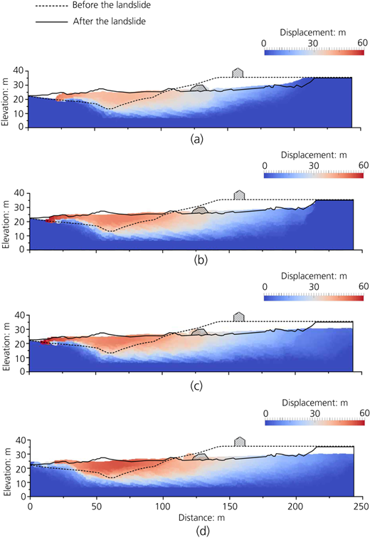
For the sake of completeness, the results of a parametric analysis performed on the influence of the shape factor λ is shown in Figure 6. Specifically, the following values of λ are considered: 20, 50, 80 and 150. In connection with this, Figure 6 shows that although the displacement magnitude does not significantly change with λ, the run-out distance and the crown retreat increase with increasing λ. In particular, the run-out distance calculated for the case in which λ = 20 is shorter than the actual one and the theoretical crown of the landslide is located approximately 10 m forward of the observed one, causing a smaller depletion zone (Figure 6(a)). The results shown in Figure 6(b) (obtained when λ = 50) better match the actual profile of the landslide body. The run-out distance is also well captured when λ = 80 and 150 (Figures 6(c) and 6(d), respectively). However, in these circumstances, the slip surface extended further upstream than what was observed, with a larger retreat of the landslide crown.
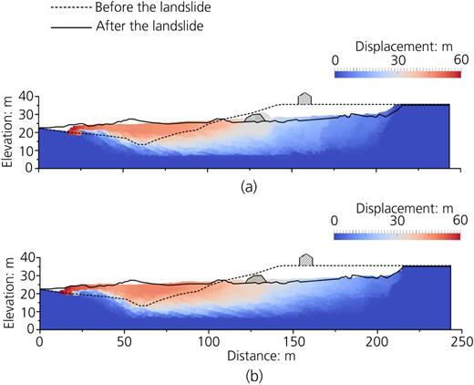
Regarding the mesh dependency on the final results, some analyses are performed using two meshes with a different size. The problem of mesh dependency when materials with a strain-softening behaviour are involved in numerical methods is well known in the literature and has been deeply investigated by many authors. For example, the problem was investigated in the field of MPM by Soga et al. (2016) and Troncone et al. (2022b). In the present study, no regularisation techniques were employed. However, to assess the mesh dependency on the final results, some analyses were performed using two meshes with a different average size (i.e. 1 and 1.5 m) for the case in which λ = 50. The associated results are documented in Figure 7, from which it can be seen that very similar results were obtained for both sizes considered. Therefore, a mesh with an average size of 1.5 m was employed in the calculations to reduce the computational costs.
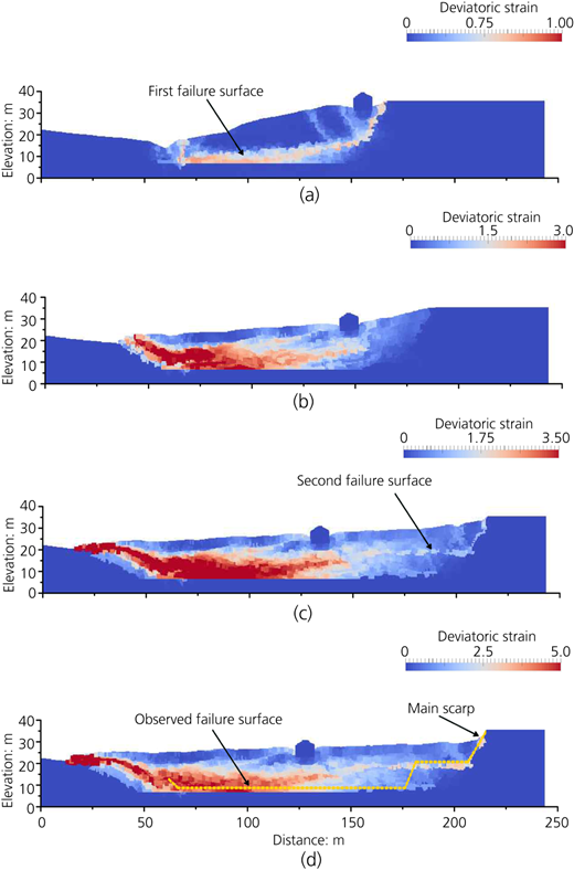
Figure 8 documents the accumulated deviatoric strains at different times to highlight the development of the slip surface and its location within the slope. These results show that the deviatoric strains concentrate in shear zones defining a failure mechanism formed by two failure surfaces.
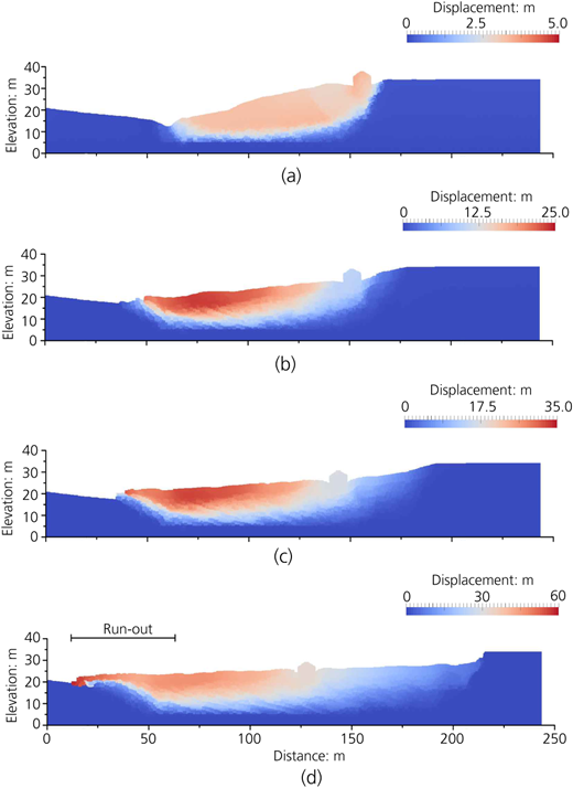
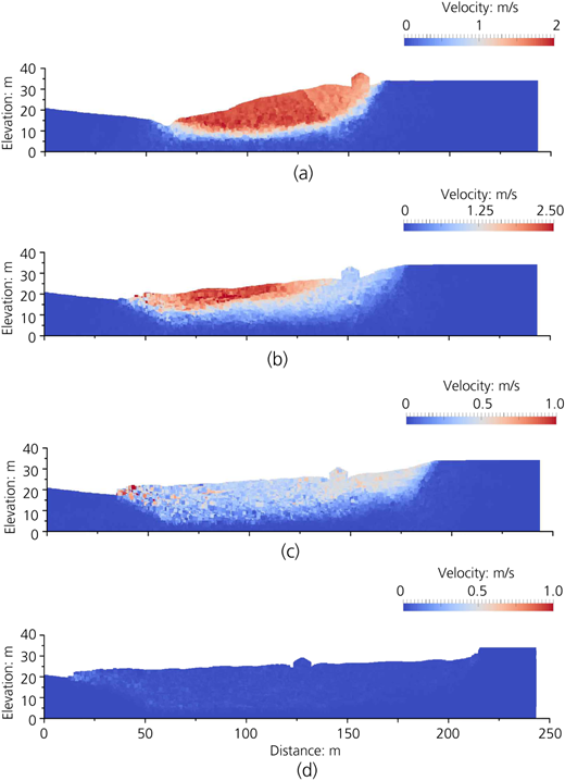
The first surface starts near the riverbed and ends just behind the existing building (Figure 8(a)). Some inclined shear zones similar to those found by Locat et al. (2017) can be also observed in the upper portion of the soil mass bounded by this failure surface. At the subsequent times (Figures 8(b) and 8(c)), the unstable soil mass moves essentially as a translational slide along the failure surface, covering the riverbed and a portion of the opposite bank. While the accumulation zone increases, the depletion zone extends upstream and a second failure surface develops at a higher elevation than the first surface, giving rise to the main scarp of the landslide (Figure 8(d)). In other words, the movement occurs in two successive phases, along two failure surfaces located at different elevations. These results are in agreement with what was observed by Locat et al. (2017), according to whom a failure surface started 2.5 m under the river elevation and propagated almost horizontally for about 100 m upstream, while a second failure surface, approximately 10 m higher than the main one, developed in the upper portion of the slope up to the backscarp. In Figure 8(d), the failure surfaces observed by Locat et al. (2017) overlap on the deviatoric strain field calculated at the end of the numerical simulation performed in the present study. As can be seen, there is a reasonable agreement between the shear zones obtained using MPM and the failure surfaces reconstructed by Locat et al. (2017). The good agreement between prediction and observation (Figures 5 and 8) also corroborates the assumption that the post-failure stage of this landslide developed under undrained conditions. Finally, the evolution of the landslide body at different times is also documented in Figures 9 and 10, in terms of total displacement and velocity, respectively. After the failure stage, the portion of the slope extending from the slope toe to the building is the first to move (Figure 9(a)). Subsequently, while the unstable soil mass continues to move downstream, invading the opposite bank of the river, the head of the landslide draws back upstream (Figures 9(b) and 9(c)) until the unstable soil mass attains a new equilibrium condition (Figure 9(d)). The maximum velocity of the material points occurs at the beginning of the post-failure stage and attains values on the order of 2–2.5 m/s (Figure 10).
Summarising, the present paper recommends MPM as an effective and very useful numerical technique for analysing landslides involving very sensitive clays, which are characterised by a very high velocity and a very long run-out distance due to a considerable soil strength reduction during the run-out process.
Conclusions
The deformation processes occurring during the failure and post-failure stages of the 2010 Saint-Jude landslide are analysed using MPM, which is an advanced numerical method capable of overcoming the limitations of the traditional numerical techniques when dealing with large deformations. This landslide is a well-documented case history with an appropriate geotechnical characterisation of the involved materials and a detailed description of the failure mechanism. The obtained results confirm the capability of MPM in properly predicting the development of the failure surface within the slope and simulating the run-out of the considered landslide under undrained conditions. In particular, although no restraint was preventively imposed to the location of the slip surface, the predicted failure mechanism is very similar to that reconstructed by Locat et al. (2017). Moreover, the final profile of the landslide body provided by MPM is in good agreement with the observed one. Some aspects concerning the kinematics of the unstable soil mass during the post-failure stage are also highlighted to complete the understanding of the deformation processes of this complex landslide. These results show that MPM is an attractive method for predicting successfully both the failure mechanism and the run-out of landslides in very sensitive clays, requiring also a limited number of conventional geotechnical parameters as input data.