Cadia dam: a critical state view of residual soil behaviour

c

critical state

r

residual (after large deformation)

s

bonded (structural) component of strength

tc

triaxial compression condition

y

yield (onset of plastic strains)

0

initial condition

1, 2, 3

principal directions of stress or strain

e

elastic

P

plastic

c

cohesion (FL⁻²)

p′

mean effective stress: 3p′ = σ′₁ +   σ′₃ (FL⁻²)

p_c

mean effective stress in the critical state (FL⁻²)

q

triaxial deviator stress: q = σ₁ − σ₃ (FL⁻²)

η

dimensionless distortional stress measure η = q/p′

σ_1y

yield stress in major principal stress direction (FL⁻²)

σ_sb

stress at onset of fabric (structure) breakdown (FL⁻²)

σ_1,2,3

principal stresses (FL⁻²)

D

dilatancy, as ratio of strain rates dε_v/dε_q

D^p

plastic dilatancy, as ratio of strain rates dε_v^p/dε_q^p

ε_q

distortional strain measure work conjugate with q: 3 ε_q = 2 (ε₁ − ε₃)

ε_v

volumetric strain ε_v = ε₁ + ε₂ + ε₃

ε_1,2,3

principal strains (assumed coaxial with principal stresses)

e

void ratio

e_c

void ratio in the critical state at current p′

ψ

state parameter, ψ = e − e_c

Η

plastic hardening modulus

M

critical friction ratio, equals η_c at the critical state. Value at triaxial compression (m_tc) taken as reference soil property

N

Nova’s volumetric coupling coefficient in stress-dilatancy

Χ

scaling factor (soil property) for state dilatancy

Γ

reference void ratio on CSL, defined at p′ = 1 kPa

λ

slope of CSL in e − ln(σ_m) space for semi-log idealisation

λ₁₀

slope of CSL, but defined on base 10 logarithms (= 2.3 λ)

Critical state theory has evolved through various contributions, some inspired by tests on sands and others by tests on clays. In the case of sands, such tests usually involved reconstituted samples (e.g. Been et al., 1991; Castro, 1969) with trends in measured strengths evolving into the state parameter approach (Been and Jefferies, 1985, although anticipated in Parry, 1958). This thread was then formalised as NorSand (Jefferies, 1993). In the case of clays, thinking has been influenced by the sustained and fundamental investigation of clay behaviour, directed by Henkel (David, 2006), using remoulded samples of London and Weald clays; Parry (1956) provides a convenient summary. This data on remoulded clays provided the inspiration, and calibration, for Original Cam Clay (OCC; Schofield and Wroth, 1968). Thus, whether considering sands or clays, a perception that critical state theory (OCC, NS, and other ‘bounding surface’ variants) applies to ‘structureless’ (remoulded) soils and thus that critical state approaches have no relevance to in situ residual soils (Wesley, 2015; this journal). A residual soil is one derived from parent rock through chemical weathering and which may retain a structure or particle-arrangement reflecting that parent rock.

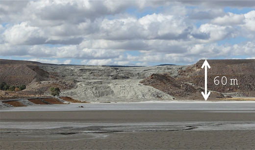
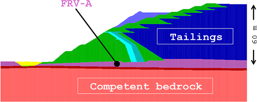
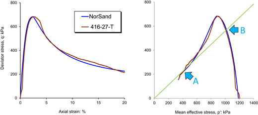
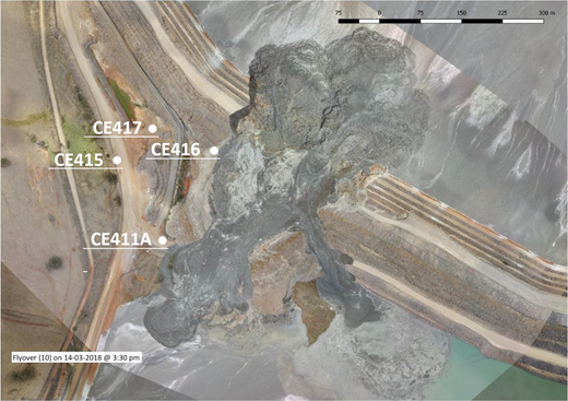
Consider Figure 1, which is an undrained triaxial compression test. The data from the test (the brown line) resembles numerous examples of static liquefaction that can be found in the literature. Static liquefaction involves the soil developing a ‘normal’ undrained strength but which is then followed by a brittle strength loss to the soil’s critical state. However, this data is from a test on residual soil – Forest Reef Volcanic unit A (FRV-A) – from the foundation of Cadia Northern Tailings Storage Facility (NTSF) and which contributed to the slump of the 95 m high NTSF embankment (Morgenstern et al., 2019; subsequently referred to as the International Tailings Review Board: ITRB). Figures 2 and 3 show views of the slump with Figure 4, a section through the centreline of the failure illustrating the FRV-A stratum.

Simply looking at the stress path and stress–strain behaviour of Figure 1 begs the question: might the liquefaction literature offer an approach to the de-structuring of natural soils with strain? The points denoted as ‘A’ and ‘B’ on Figure 1 have particular significance to this idea and will be discussed after describing the geological origin of the soil and its physical properties. The blue line on Figure 1 is the stress–strain behaviour and stress path computed using the extended version of NS developed in this paper to capture residual soil behaviour.

The inclusion of structure within a constitutive idealisation of soil has often been informed by ideas from the Cam Clay framework (Schofield and Wroth, 1968; Roscoe and Burland, 1968). Remoulded behaviour is treated as a reference configuration defining the relation between void ratio, stress, and the onset of yield. Soil structure moves the remoulded yield surface ‘outwards’ to increase the yield stress – in effect, adding an apparent pre-consolidation pressure even though that pressure is unrelated to loading history (Burland, 1990). As an example, compare Cotecchia and Chandler (2000, their Figure 7) with Schofield and Wroth (1968, their Figure 6.5). There are variations on this approach, e.g. moving yield in the direction of void ratio rather than adding a pre-consolidation pressure, but these variations are intrinsically similar in principle.

Expansion of a remoulded reference configuration to capture structure leads to an increased elastic region (because the yield surface is pushed outward), but residual soils yield with plastic strains before this expanded surface is encountered. A response to this shortfall has been to introduce either non-linear elasticity (e.g. Jardine et al., 1986) or multiple and nested yield surfaces (e.g. Mroz et al., 1979). There are also other contributions along these lines which may fit particular tests. Liu et al. (2000) provide a thorough explanation of these developments in relation to ‘structured’ soils. Most generally, nested yield surfaces and non-linear elasticity are compensating for underlying conceptual errors and the appropriate start is to go back to the underlying mechanics.

Cam Clay (both Original and Modified) assumes that the yield surface always intersects the critical state locus. This is both unnecessary and, in general, incorrect. This deficiency affects prior work on capturing soil structure that has been informed by Cam Clay (or which retains elements of the Cam Clay framework). The unnecessary aspect of Cam Clay is removed by invoking the central premise, tracing to Casagrande (1936, 1975), which is that soil moves to its critical state with deformation. There is no requirement that the yield surface must intersect the critical state locus (in e-p-q space) in general. Casagrande’s concept can simply and formally be expressed using the state parameter ψ (ψ = e − e_c) and which gives ψ => 0 with distortion. NorSand (Jefferies, 1993) adopts this idea by decoupling the yield surface from void ratio and capturing a range of soil behaviours using very few soil properties. The question then becomes: how might NS be modified to include the particular characteristics of residual soils?

When soil strength was first considered in terms of effective stress (Terzaghi, 1943), the Mohr–Coulomb strength model was modified to use the properties c′ and ϕ′ in what is now referred to as the Terzaghi strength model. Taylor (1948) demonstrated that the Terzaghi model did not account for a substantial effect of dilation (referred to as ‘interlocking’ at the time) on soil strength, but gave no equation for this. Bishop (1950) provided the mathematical representation of Taylor’s idea with strength now having the properties of critical state friction angle ϕ_c, a dilation angle δ, and no cohesion. This Taylor–Bishop idea underlies modern theory of soil behaviour and critical state soil mechanics. In particular, NS was derived using the Taylor–Bishop strength model. Christian and Baecher (2015) provide an interesting history of this evolution of ideas.

The vulnerability of residual soils to structure breakdown in oedometer tests is well known (e.g. Wesley, 2013) with the related notion that breakdown develops as a consequence of vertical stress. The extension introduced herein is to treat residual soil structure as a true cohesion (bonds between the soil particles), with that cohesion decaying after a certain distortional strain. The preference for distortional strain is because it is this strain that causes the evolution of particle arrangement; a concept proposed by Reynolds as early as 1885. Oedometer tests include distortion even though the test is usually considered in terms of vertical stress. This extended notion of structure degradation allows the strength and stiffness of residual soil to be represented by a minor modification of stress-dilatancy within critical state theory, thus avoiding the difficult problem of identifying specific parameters using physical tests on inherently variable residual soils (particularly when investigation resources are limited and/or time being of the essence in finding a workable solution). A particular attraction of this approach is that it allows existing geotechnical modelling packages to be used to simulate progressive failure of residual soils, with the only restriction being that the chosen package must allow ‘scripts’ to update the critical state stress-ratio M at the relevant gauss points as the analysis proceeds (e.g. a FISH routine in the case of Itasca software).

We have adopted the following terminology to capture all aspects of residual soil within the framework of plasticity theory:

• Yield stress is where plastic strains develop and is denoted by the subscript ‘y’. Yield stress evolves during plastic deformation, tracking the current stress. Peak strength is not ‘yield’, as it is sometimes called in the literature (in work-hardening plasticity theory, peak strength is an ‘output’ of the theory not a soil property).

• Over-consolidation ratio (OCR) does not imply or measure past loading history, but reflects the current stress-state to the stress-state where yield arises; in the case of an oedometer test, for example, OCR = σ′_vy/σ′_v. There may not be a correspondence between geological past maximum stress and mechanical yield because yield also develops during ‘unloading’ and which reduces the yield stress (Jefferies, 1997).

• The stress at which the stiffness and or strength begins to degrade is denoted by the subscript ‘sb’ (for structure breakdown). As will be illustrated, at the outset of loading the residual soils considered, σ_sb ≫ σ_y.

• The residual strength is a large strain condition as observed in the test data and denoted by the subscript ‘r’. It may or may not involve shear planes or preferential particle orientations.

• The critical state is where structure breakdown is complete and the residual soil is now essentially reduced to an assembly of particles without any bonds where deformation can continue without further changes; this is denoted by the subscript ‘c’. The critical state is taken as the same as the residual state as, for the soils considered here, that appears to be the case.

The FRV is the dominant rock type in the vicinity the Cadia NTSF slump. The FRV comprises a thick (2.5 km) sequence of mafic to intermediate volcanic rocks, sedimentary breccias and lesser sandstones intercalated with basaltic andesite and andesitic lavas. Deposition of the FRV spanned the Late Ordovician to Early Silurian (≈420 Mya). Following uplift and erosion of the FRV (and overlying strata where present), the FRV was exposed to an extended period of deep chemical weathering during which time a residual soil profile developed under a paleo-climatic regime that was warmer and more humid than the present. At the same time, alluvium (paleo-alluvium) was deposited locally along drainage lines.

During the Tertiary (≈10 Mya) the weathered surface and paleo-alluvium (where present) was unconformably overlain by basalt which flowed from the north following the drainage lines where its thickness was greatest. After the late Miocene much of the basalt and upper FRV weathering profile was eroded, leaving the thicker remnants of basalt (formerly along drainage lines) now along ridges. One such remnant formed a low ridge immediately to the west of the NTSF slump.

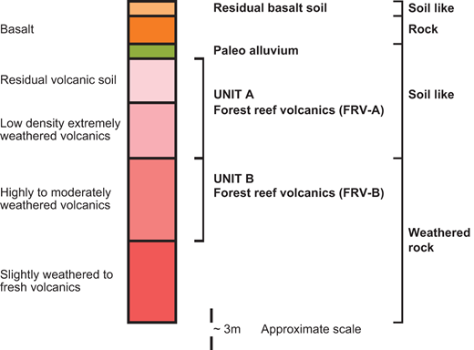
Where the basalt had either prevented or inhibited the physical erosion of the FRV weathering profile it was found that the upper section, designated as FRV Unit A (FRV-A) was preserved. This material had a significantly higher void ratio and lower density compared to the lower section or the weathering profile well away from the basalt, designated as FRV Unit B (FRV-B).

The stratigraphic profile immediately west of the NTSF embankment failure is summarised in Figure 5. Further background on this geological model for the Cadia foundation can be found in the ITRB report as well as Gordon and Wates (2024).

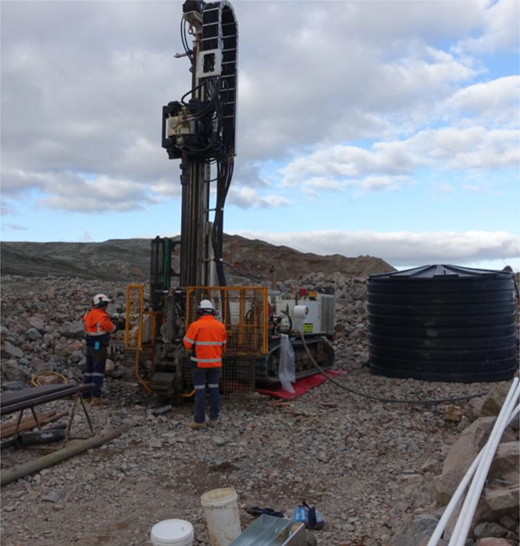
Investigation of the NTSF embankment and embankment foundations in the vicinity of the slump was undertaken using a Boart Longyear LS250 MiniSonic drill (Figure 6) capable of both sonic and rotary drilling. Apart from being the preferred drilling technique in embankment dams, sonic drilling was necessary to: 1) quickly penetrate the substantial depths of rockfill in the body of the dam and containment berms that were constructed following the slump; and 2) enable large diameter samples of residual soils and weathered rock to be taken for testing.

In several drillholes, near-continuous recovery of foundation soils and extremely weathered rock was achieved using a clear polycarbonate (Lexan) liner inside a 1.5 m long sonic split barrel. The liner had an outer diameter of 108 mm OD, a length of 1521 mm, and a wall thickness of 3.2 mm. The Lexan samples were cut into 500 mm lengths using a hand saw, classified and then sealed and protected for transport prior to testing. In the laboratory the Lexan liners were split and the sample then trimmed to 63 mm dia. for testing. Trimming the sample assisted in removing potential disturbance to the test specimen.

Undisturbed stainless steel thin-walled samples (63 mm dia. and 500 mm length) were also pushed from the bottom of drillholes in residual soils, paleo-alluvium and extremely weathered rock using the sonic drill string as a casing. In the laboratory these samples were extruded from the thin-walled sample tube.

FRV-A was identified in several drillholes located to the west of the slump where the basalt afforded protection from physical erosion. Triaxial test results on samples presented herein come from two of these drillholes, CE415 and CE416. These drillholes, together with other holes where FRV-A was intersected are shown on Figure 2. Evidence that FRV-A daylighted to the east of the basalt and beneath the slump comes from a bulk sample taken from the embankment toe prior to the slump, however the slump has removed further evidence of FRV-A in this area.

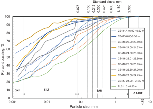
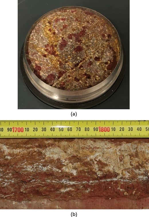
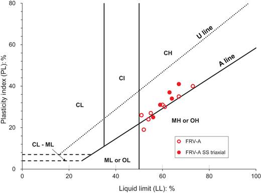
In the field, FRV-A presents as a very stiff to hard, medium to high plasticity, red orange to brown clayey silt with white or purple speckling and/or veining. Hand penetrometer readings on the ends of undisturbed samples typically registered in the range 300–400 kPa. The recovered samples of the FRV-A showed well-graded distributions of particle sizes for all samples with substantial changes in those distributions from one sample to another (Figure 7). The index properties, Figure 9, are correspondingly scattered and amount to the FRV-A classifying as just clayey of an MH silt regardless of individual sample gradation. Triaxial test samples presented in this paper (highlighted on Figure 7 with thicker lines) are generally the finer particle size distributions. Figure 8(a) shows a tube sample, after extrusion and trimming for a direct simple shear test, with typical speckling, while Figure 8(b) shows white kaolinite veining in a split Lexan tube.

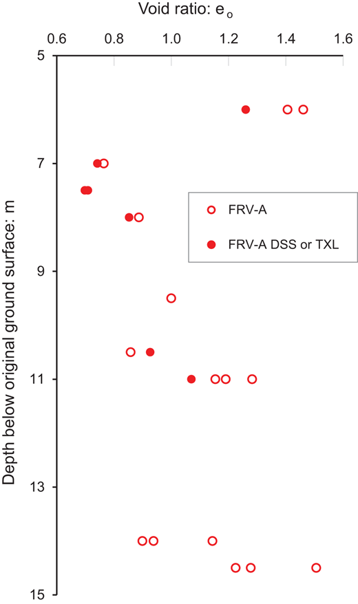
In sedimentary rocks and alluvial soils, the void ratio depends on the packing of individual grains. In residual soils derived from igneous rocks (where the void ratio of the parent material is essentially zero), the void ratio results from the change and loss of mineral constituents due to chemical weathering and the preservation of relic mineral structure. The in situ void ratio of the weathered FRV-A was assessed from the water content and specific gravity of the recovered samples and the data is shown on Figure 10. The in situ void ratio (e₀) is high for such a well-graded soil, with numerous e₀ > 1.0, indicating a very open relic structure. The triaxial tests were carried out on a broad range of void ratios observed for the FRV-A.

All the foundation strata at Cadia were tested for their mechanical properties. Here we focus on the FRV-A as it exhibits the most extreme brittle post-peak strength loss both in terms of the magnitude of strength loss and that rate of that loss with strain. This was considered a controlling factor that resulted in slumping of the NTSF (Morgenstern et al., 2019).

Strength tests undertaken on FRV-A were mostly direct simple shear (DSS) tests. DSS tests were preferred because the limited thickness of the FRV-A overlying competent bedrock at the slump most likely resulted in simple-shear deformation of the FRV-A in the field. However, DSS data is not helpful in terms of understanding fundamental behaviour as neither of the horizontal normal stresses are measured. Thus, the DSS testing was supplemented by seven single-stage consolidated undrained triaxial compression tests with pore pressure measurement (CIU) which are listed in Table 1. Four of these tests were by one laboratory (TriLabs, Brisbane) and three by another (Golder, Perth), providing a check on the repeatability of the data.

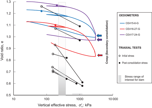
Three controlled rate of strain (CRS) oedometer consolidation tests were completed (Golder, Perth) and these are listed in Table 2. These tests followed ASTM D4186 procedures. The oedometer compression data is presented in familiar semi-log form on Figure 11. All samples show a similar pattern of behaviour typical of many residual soils: a strongly curved semi-log plot with no clearly defined quasi pre-consolidation or vertical yield pressure exactly as noted by Wesley (2013). Accordingly, the compression index under initial loading varies with stress-level and can be characterised by C_c = 0.06 at 400 kPa, C_c = 0.075 at 800 kPa and C_c = 0.09 at 1200 kPa. One unload–reload loop test from ≈400 kPa was completed for each oedometer test, giving an average recompression index C_r ≈ 0.018; a rather stiff result but consistent with field observations. The in situ stress for the CRS samples is highlighted with a ‘diamond’ marker in Figure 11; the unload–reload loops also confirm that first-compression (i.e. plastic strains) were occurring from less than 100 kPa and likely from the outset.

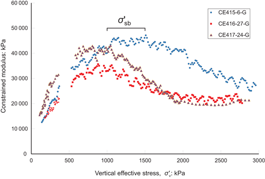
Wesley (2015) asserts that the semi-log representation of oedometer data as used in Figure 11, and thus the associated soil property C_c, is an artificial construct which is misleading for residual soils. However, if stiffness is proportional to confining stress, then void ratio will vary logarithmically with confining stress as a mathematical consequence. Thus, insight into the behaviour of FRV-A under one-dimensional vertical loading can be gained by a study of the constrained modulus during initial loading, Figure 12, and its dependence on stress. All three samples show a similar linear increase in stiffness at confining stress between ≈100 and ≈400 kPa, with a near-linear trend resuming for ≈500 to ≈700 kPa after unload–reload cycles. The behaviour then changes at confining stresses between ≈1000 and ≈1500 kPa, with the stiffness of the samples decreasing with increasing stress; a trend indicating a breakdown of the relic structure within the samples. Thus, we associate 1000 kPa < σ_sb < 1500 kPa for the tested samples and emphasise that this stress-range is not σ′_y as irrecoverable strains developed from the start of these tests. Apparent creep of between 0.8% and 2.0% axial strain was also observed at the maximum vertical stress applied, implying further collapse of the soil structure. Rebound of the samples from the maximum stress shows a different slope to the unload–reload cycle from 400 kPa, also implying a change in the soil structure through plastic yielding.

Triaxial compression tests followed the protocol of consolidating to a mean stress in excess of the in situ vertical stress before subsequent undrained shear. This is a common procedure to remove the effect of disturbance resulting from extrusion and trimming of the sample in the laboratory as well as that caused by sampling itself. The results of such tests are presented as strength ratios, in particular that of s_u/p′₀ (where p′₀ is the mean effective stress prior to shear, not the in situ value). In the case of the tests reported here, the ITRB required data corresponding to the dam loading not the less-stressed toe area (see Figure 2). The void ratio change that occurred during this consolidation was measured, with Figure 11 showing the in situ (open marker) vs as-tested condition (solid marker). With the exception of one test (416-27-T), the triaxial consolidation data exhibited a consistent average compression index slightly greater than that observed in the oedometer data, indicating minimal sample disturbance. Test 416-27-T showed much more compressible behaviour than the other tests which is thought to have been caused by disturbance.

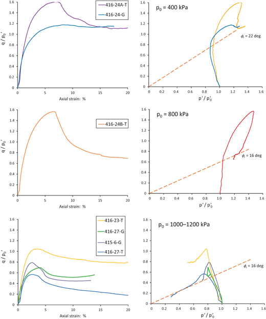
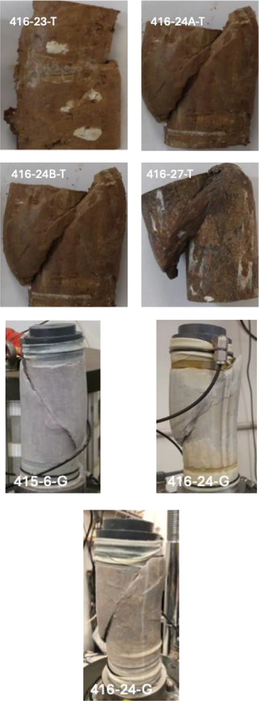
The triaxial compression data has been corrected for evolution of cross-section area during deformation. Most samples eventually failed on a shear-plane with only one (416-23-T) tending to a bulging failure; photographs of the failed samples are provided in  Appendix B. The area-corrected triaxial compression data is presented on Figure 13, normalised by the initial effective confining stress. The data has been grouped by initial confining stress, with obvious changes in behaviour.

The two tests with p₀ = 400 kPa dilated strongly after slight initial contraction and both came to the same large-strain strength that is equivalent to ϕ_r = 22°. One test (416-24A-T) showed a substantial peak strength before brittle strength-loss while the other (416-24-G) simply developed its critical state strength early.

The four tests at 1000 kPa < p₀ < 1200 kPa were broadly similar, with slight contractive behaviour to peak strength which was then followed by differing brittle strength loss. Three of the four tests developed ϕ_r = 16° with the remaining test being considerably stronger.

The single test (416-24B-T) from p₀ = 800 kPa showed marked dilation similar to the tests with p₀ = 400 kPa. The peak strength was then followed by a substantial brittle strength loss to ϕ_r = 16° as seen in the p₀ > 1000 kPa tests.

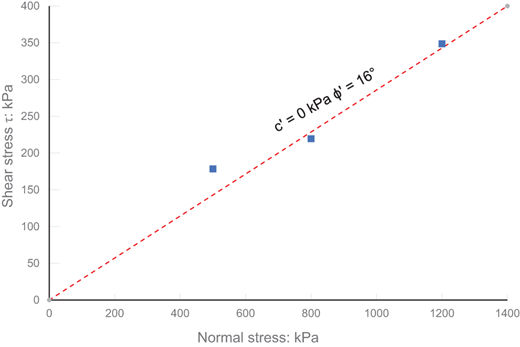
A further investigation of the residual strength used direct-shear tests on a single sample of FRV-A (CE416 24.5–25.0) remoulded at its in situ moisture content (34%) and dry density (≈1.40 t/m³). The direct shear test was completed at three normal pressures, with residual values (after 4–5 reversal cycles) indicating an average ϕ_r = 16° as shown in Figure 14. This residual strength is consistent with five of the seven triaxial tests with the other two being stronger (Figure 13).

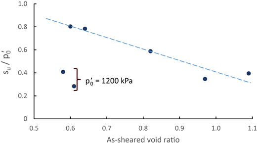
The triaxial data is summarised on Figure 15 as normalised undrained strengths. The data shows a linear trend to decreasing peak strength with increasing void ratio, with the exception of two outliers. Both the outliers had been consolidated at confining stresses of p′₀ = 1200 kPa which was in the zone of structure breakdown inferred from the oedometer behaviour (see Figure 12).

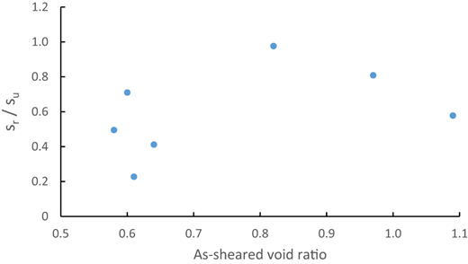
Brittleness is more difficult to quantify as two tests appear to have not reached their residual value within the limits of the triaxial tests. Nevertheless, taking s_r as the lowest post-peak value gives the undrained strength ratio s_r/s_u, as illustrated on Figure 16. The brittleness as expressed by the ratio s_r/s_u appears unrelated to void ratio.

Critical state theory is based on soil strength comprising two components: ‘friction’ and ‘interlocking’. Friction is seen as the true mechanism for dissipation of plastic work (the soil property M) while ‘interlocking’ reflects the kinematics of how the soil’s particles must move as the soil deforms and which results in a limiting dilatancy, D_min (‘min’ because of the compression positive sign convention). The strength model has the general form:

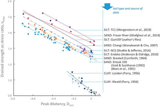
where N represents the work increment not dissipated by distortional strain. The parameters M, N are soil properties and perceived as constant in triaxial compression conditions. Strength data across a wide range of soil types and densities, ranging from clean sand, through silts, to clays has been collated and is shown on Figure 17 to illustrate that [1] represents soil strength trends regardless of soil gradation; the only effect of soil type is on the numerical values of M, N.

Equation [1] describes ‘strength’, giving the bounding (or limiting) stress ratio ƞ_max in terms of the dilatancy that the soil can develop. Starting with Original Cam Clay (Schofield and Wroth, 1968) Equation [1] has been generalised as the basis of flow rules within the theory of plasticity as applied to soils – it is near ubiquitous across modern constitutive models (although notation varies) and can be expressed in the stress-dilatancy form:

where ƞ is the current ratio of deviatoric to mean stress and D^p is the corresponding ratio of the plastic work-conjugate strain rates. This equation generalises to 3D and is not restricted to triaxial compression.

Referring back to Figure 1, the green dashed line on the stress path of this figure has been fitted to the end-of-test conditions, matching the stresses measured at large strain, namely, point ‘A’ on the figure. The gradient of this line is M_r = 0.62 (‘r’ for residual) and is the large-deformation value, with this M_r corresponding to ϕ_r = 16°. Point ‘B’ on the figure is the intersection of this large-deformation strength ratio with the undrained stress path at about 2% axial strain. At this point the sample had mobilised only about half of its peak strength. For incompressible pore water (the usual assumption), the elastic-plastic strain decomposition gives the mean effective stress change during an undrained plastic strain increment as:

where K is the elastic bulk modulus of the soil and dε_q the deviatoric strain increment (which is the same as the dε₁ for undrained triaxial compression). Looking at point ‘B’, the stress path direction (i.e. dp′ < 0) implies D^p > 0 at B (since this is a compression test with increasing deviator strain and K is positive).

In the case of Equation [2], experimental data is that 0 < N < 0.5 for clays, silts, and sands during triaxial compression (Jefferies, 2021), while there is the possibility that N might become negative during unloading (Jefferies, 1997). Neither of these cases produces a negative denominator. Thus, D^p > 0 requires M > η and at B, M > M_r.

More generally, and contrary to conventional critical state theory, M is an evolving property:

where M_r is the residual or true critical state value while M_s captures soil structure and evolves. While it might be usual to see soil structure as an overall expansion of the yield surface (e.g. the various approaches discussed by Liu et al., 2000), that view does not fit the measured stress path for the FRV-A which indicates plastic yielding from the start of compression (elastic stress paths are purely vertical on a p–q plot); and, is also consistent with the oedometer data (Figure 12). A true cohesive strength ‘c’ is indicated, with the soil’s yield surface expanded in the ‘q direction’ but without comparable expansion in the ‘p direction’.

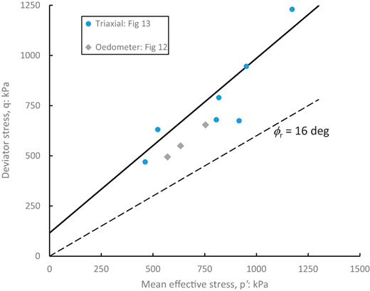
The stress conditions at which structural breakdown (brittle strength loss) developed in the triaxial tests (the vertex on the stress paths) are shown in Figure 18. This figure also includes the breakdown identified in the oedometer tests (Figure 12), with that data being plotted assuming K₀ = 0.5. There is both a clear cohesive element to the structural strength and an enhanced frictional element, the latter being about 50% stronger than the residual value. On average, across the range of void ratios tested, the fitted trendline corresponds to structural breakdown developing when:

where stresses are in kPa. For M_r = 0.6 (16°) and normalizing 5a by p′, the structure-related strength can be expressed as:

The measured post-peak strength loss is somewhat similar to static liquefaction of a loose sand, but with a more abrupt loss immediately post-peak. It was hypothesised that a negative exponential decay of M_s would be appropriate and starting from peak-strength (a reference strain cannot be used for analysis of a boundary value problem). The form adopted was:

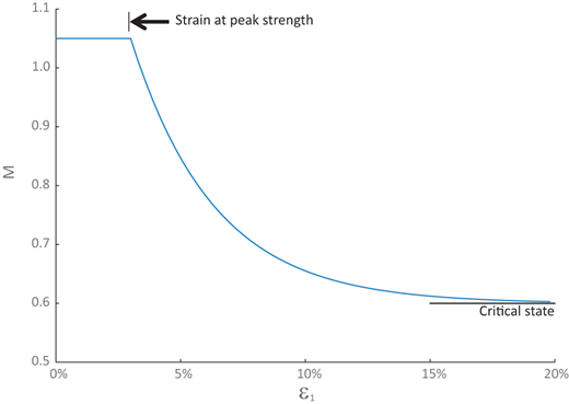
where $εqf$ is the deviatoric strain at peak strength. The parameter $α$ in [6] is a coefficient that represents the rate of decay of the soil structure (i.e. the cohesion c) with strain, with Figure 19 showing the form of [6]. The post-peak fit of NS to the data, the blue line on Figure 1, was computed using this idealisation and with unchanged soil properties from those used to calibrate to the peak strength and initial stiffness.

Despite what appears to be very different strengths and compressibility, the physical and mathematical representation of sand and clay behaviour has a common framework when a soil’s CSL is used as a reference state. State-based models represent a long-established framework for understanding mechanical aspects of soil behaviour using work-hardening plasticity with substantive contributions from both the USA and the UK (see Jefferies and Been, 2015 for a historical perspective). NorSand (NS) was the first of these state-based models and its equations are summarised on Table 3. NS accurately captures the entire spectrum of soil behaviour from dilation of dense soils through to extreme liquefaction of very loose ones. The soil properties used in NS are largely familiar, see Table 4, and with the exception of the plastic modulus H are not specific to NS. The version of NS used here excluded the ‘softening term’ and this corresponds to setting the parameter S = 0 in commercial implementations. All properties are determined by triaxial compression tests.

The further aspect added for capturing the FRV-A behaviour is the introduction of c, α so that M_tc in ‘standard’ NS becomes replaced by Equation [6]. If c = 0, then standard NS is recovered.

The range of gradations encountered in the FRV-A (Figure 7) makes each of the seven triaxial tests a test on a particular material. Thus, properties will vary from test to test.

The slope of the CSL was assumed to parallel the compressibility measured in the oedometers (i.e. λ₁₀ = C_c) and thus using the values discussed earlier. There was no assessed effect of initial void ratio on compressibility, but increasing compressibility with increased confining stress was adopted.

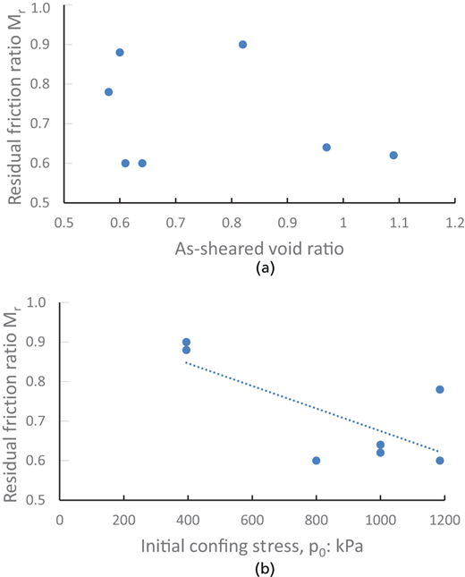
The large-deformation ‘frictional’ strength (i.e. M_r) was determined by inspection of the measured data and corresponds to Point A in Figure 1 in each test. This is formally denoted as a residual value. The values vary from test to test and are in the range 0.6 < M_r < 0.9, with no clear effect of void ratio (Figure 20(a)) but with a tendency to reducing with increasing confining stress at the start of shear (Figure 20(b)).

There is no other direct determination of soil properties. Iterative modelling was required to infer the full set of FRV-A properties.

There are six soil properties in ‘standard’ NS (Table 3) with two further properties (cohesion, and rate of loss of cohesion) added for representing residual soil. Some of the properties are known directly from test data, with the others obtained by iterative modelling. Iterative modelling involves estimating the soils properties and using those to compute the full stress–strain behaviour. The computed stress–strain behaviour is then compared to that measured, with estimates then being updated to improve the fit between simulation and data. Iteration continues until an acceptable match is obtained. The details of the iterative modelling are given in  Appendix A.

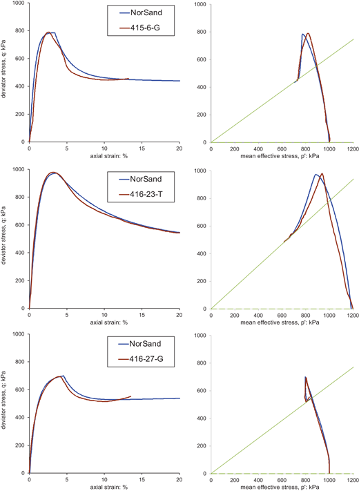
There are four tests within this range of p′₀, and all four showed contractive behaviour. Iterative modelling was well-constrained and there was little difficulty in achieving fits. One test was shown in the Introduction (Figure 1) with the other three tests shown on Figure 21. The properties that gave these fits are presented in Table 5a while Table 5b documents the inferred as-tested state of each sample. Interestingly, while three tests exhibited plastic yield from the outset (typical of a normally consolidated state), sample 416-27-G (the bottom plot of Figure 21) showed an initially vertical stress path that indicates no plastic strains for the first part of loading and as a consequence a small over-consolidation (OCR = 1.15) was added to capture this behaviour.

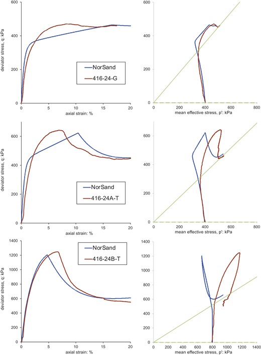
There are two tests that were consolidated to p′₀ ≈ 400 kPa and one further test consolidated to p′₀ ≈ 800 kPa. All three tests dilated to peak strength, with the change from contractive to dilative behaviour arising at approximately M_r (the green line on the stress path plots of Figure 22); this is the opposite behaviour to the samples tested with p′₀ > 1000 kPa (Figure 21).

Although both tests at p′₀ ≈ 400 kPa developed a ‘peak’ undrained strengths, the test from p′₀ ≈ 800 kPa moved to a structural breakdown while q was still increasing. In all three cases the best-fit NS simulations had dq/dε₁ > 0 at the observed onset of breakdown which prevented the criterion dq/dε₁ = 0 being used to define this onset; therefore, a maximum value of q was input as a criterion to trigger the transition into [6]. The fitted behaviour is shown in Figure 22, and the properties used are given in Table 5.

Overall, while the fits to stress–strain vary from ‘not unreasonable’ (the tests at 400 kPa) to ‘good’ (the test at 800 kPa), the computed stress paths diverge from those measured. The divergence of computed behaviour from that measured arises when η > M_r (i.e. when the stress paths goes above the green lines in Figure 22). The computed paths invoke [5] and thus are contractive to near peak-strength. It is unclear whether the divergence is caused by anisotropic elastic moduli (neither measured nor implemented in NS) or by a form of non-associated behaviour where ‘strength’ is decoupled from dilatancy (say using M for strength but M_r for dilatancy; a theoretical basis for this is unclear).

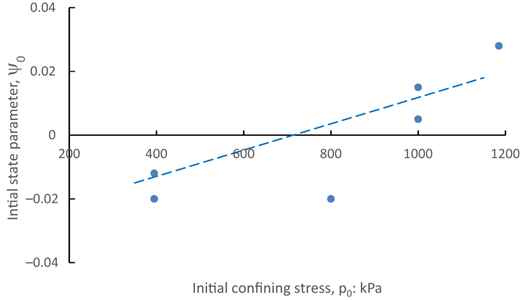
The initial state parameter ψ₀, and, to a lesser extent, the OCR are the key metrics for a critical state approach. Here the fact that the FRV-A is a residual soil (without a pre-consolidation pressure as such) leads to expected plastic yield from the outset, reflected in OCR = 1 which positions the yield surface onto the initial stress state (with one minor exception, 416-27-G, where OCR = 1.15 was used). In the case of ψ₀, this would normally be assessed from CPT data and/or the combination of measured void ratio combined with the measured CSL. No CPT were attempted in the FRV-A, and the CPT-based procedure has only been established for unbonded soils. The wide range of gradations prevents inference of the multitude of CSL’s, and thus measured void ratios are not in themselves useful. However, it is intriguing to consider the inferred ψ₀, from simulating the various undisturbed tests with their initial confining stress (Figure 23). There is both a consistent limited range of initial states and with the familiar trend of becoming less dilatant with increasing confining stress. A ‘design characterisation’ is clearly possible given some undisturbed samples (as was the case at Cadia). Although we suggest a linear fit in Figures 23, a bi-linear characterisation might be plausible with a ‘pivot’ at about 900 kPa which is intriguingly close to the ‘structure breakdown’ pressure. More research was not possible within the ITRB scope.

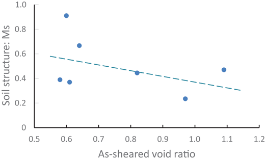
The suggested framework for the brittle behaviour is a cohesive component reflecting relic bonds that is lost after peak strength, with this cohesive component captured in stress-normalised form by the parameter M_s (as per [5]). The values shown on Figure 24 are those realized in the simulations, reflecting the computed excess pore pressure. There may be a weak trend to relic-bond strength decreasing with increasing void ratio (Figure 24).

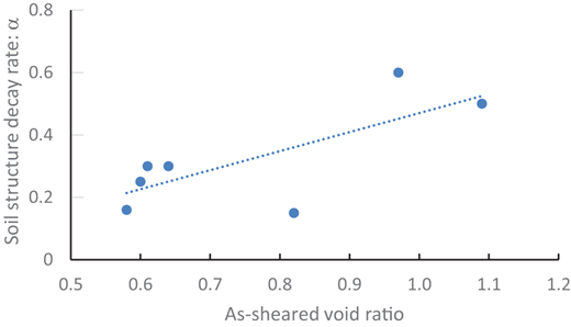
The decay from peak strength to residual (= critical state) strength was modelled by an exponential decay controlled by the rate-parameter α. The calibrated decay rates are shown in terms of the initial void ratio on Figure 25, with looser void ratios causing faster loss of bonds with strain (i.e. bonds are more easily broken if the soil is loose).

Overall, the trends seen in Figures 23–25 suggest that using a critical state approach is not unreasonable for the FRV-A. The fit of the theory to data is excellent for the four contractive tests and ‘intriguing’ for the three dilating ones.

The undrained behaviour of the residual soil that was the most significant controlling factor that resulted in slumping of Cadia’s NTSF, the FRV-A, has been evaluated using the framework of critical state theory. An extension of that theory, the inclusion of true cohesion within stress-dilatancy, is indicated from inspection of the measured stress paths in triaxial compression. The extension is a straightforward modification of NorSand requiring two new properties: the cohesion itself, c, that represents the relic bonds and, a parameter, α, representing the rate of destruction of that cohesion with distortion. There are seven relevant single stage triaxial tests on residual soil within the database from the Cadia failure investigation and all are captured using the extended theory. The two new parameters introduced (c, α) show intuitively sensible trends within the geological understanding of this residual soil. The authors suggest that this modification to NorSand will provide a convenient means of modelling the coupling of brittle failure in TSF foundation soils to the triggering of static liquefaction in contained tailings, a situation that developed at Cadia NTSF.

The triaxial data used is public-domain and can be found in the ITRB report (Morgenstern et al., 2019, their Appendix D). This data has been modelled using Excel, with routines written in VBA (i.e. as a macro-enable file). Although this format is blocked for posting on the journal website, interested readers are welcome to contact author² for a copy of this modelling workbook which is open-code, so the routines are readily viewed.

There are six soil properties in ‘standard’ NS (Table 3) with two further properties (cohesion and rate of loss of cohesion) added for representing residual soil. Iterative modelling becomes more effective as the parameters iterated are reduced. Accordingly, three properties were estimated from other evidence and not iterated: Ν, χ, ν.

Nova’s coefficient N is best defined using a range of drained triaxial compression tests on dense samples, which do not exist for Cadia. However, N ≈ 0.35 has been commonly encountered across a wide range of soil types and this was adopted.

Poisson’s ratio is rarely measured in geotechnical engineering, and only enters consideration as it links G to K with K being the truly important property as K controls much of the undrained response via ref. [3]. Based on Bellotti et al. (1996), ν = 0.2 was adopted.

The state dilatancy coefficient χ physically reflects the difficulty of soil particles moving in response to imposed distortion. As such, more compressible soils (clays) show smaller values of χ than less compressible soils (sands). Equally, uniformly graded soils show smaller χ than well-graded soils. These two considerations led to the choice χ = 4 as ‘not unreasonable’; in essence discounting the effect of the clay fraction within the FRV-A because of its well-graded nature (Figure 5).

Some aspects of iterating are straightforward with little ambiguity. For a semi-log CSL, the ratio of critical state mean stress (p′_c) to the initial mean stress (p′₀) is an exponential function of the ratio ψ/λ. Thus, this ratio controls the extent of the undrained stress path. In the modelling shown here it was assumed that the CSL and the NCLs for the FRV-A were parallel and so λ₁₀ = C_c, with C_c varying with the consolidation stress. In turn, this makes ψ₀ well-constrained in modelling any test.

A complicating factor is that there is a wide range of gradations within the FRV-A, and thus some properties will vary from place to place within the stratum and thus between the undisturbed triaxial samples. The ‘altitude’ of the CSL (Γ) is one property that varies from place to place; it was determined for each of the tested samples by using the inferred state parameter and the measured void ratio of the sample. Likewise, the true cohesion c will vary from place to place because of non-uniform weathering, but this property dominates the computed s_u => s_r change and thus is well-constrained. Similarly, the rate of this s_u => s_r change substantially constrains α.

The stress path is strongly influenced by the ratio of elastic to plastic stiffness through ref. [3], that is, the ratio I_k/H. Equally, the stress–strain stiffness to peak strength is strongly influenced by H. Iteration balanced these two contrasting effects to fit NS to each test with clear values of both I_k and H.