
It is sometimes convenient to treat a relatively rigid footing as a single element subjected to up to six force resultants: vertical load, horizontal load in two directions, overturning moment about two axes and torsion. Applications include calculations of initial, elastic settlement; foundation responses under seismic loading or for machine vibrations; and fixity of an offshore jack-up foundation under cyclic wave loading. Present codes of practice provide formulae that assume fully isotropic and linear elastic soil and in some case assume no friction between the footing and soil. This paper uses recent theoretical advances to develop solutions for stiffnesses of rigid circular footings on transversely isotropic linear elastic soil, including with interface friction. Closed-form solutions are developed for vertical load and overturning moment on a frictionless interface and for vertical load and torsion on a frictional interface. A boundary-element analysis is presented for the cases of lateral load and overturning moment on a frictional interface. By fitting expected forms to the results, new formulae are proposed for stiffnesses for these cases. The effects of interface friction on limiting loads are calculated. Practical applications are outlined, and some limitations are briefly discussed.
Notation
Principal stress and principal strain are taken as positive in compression. Moduli and Poisson’s ratios are effective drained parameters. ‘Vertical’ means parallel to the axis of material symmetry, and ‘horizontal’ means at 90° to the axis. The z-coordinate axis points vertically downwards. Footing displacements v, h, Bξ and BΩ; are small displacements of the centre of the footing at the soil–footing interface, with ξ and Ω being angular. Generalised loads V, H, M/B and T/B are force resultants referred to that point, with M being the overturning moment and T being the torque. Angles are positive clockwise in plan view. An integral sign without limits refers to integration over the circular soil–footing interface, normalised or otherwise as in context.
- a, b
miscellaneous constants, defined where used
- Aij
constrained modulus, notation by Liao and Wang (1998)
- B
footing diameter
- C
(with letter subscripts) footing system compliance factor
- Cij
(with number subscripts) constrained modulus
- cA, cP
cosines
- d
infinitesimal
- d
dense
- da, da′
infinitesimal area and normalised version, da′ = 4da/B 2, respectively
- Eh, Ev
drained (effective) Young’s moduli in the horizontal and vertical directions
- f
factor or function, defined where used
- G
shear modulus (un-subscripted for a fully isotropic linear elastic (FILE) material, subscripted for a transversely isotropic (cross-anisotropic) linear elastic (TILE) material)
- Ghh
modulus for shearing in a plane at 90° to the axis of material symmetry
- Ghv, Gvh
modulus for shearing in a plane containing the axis of material symmetry, G hv = G vh
- H
horizontal force resultant on the soil–footing interface area
- h
footing displacement in the +x direction
- K, K′
stiffness (units of force over length) and dimensionless stiffness, respectively
- k′
dimensionless factor involved in calculating footing system compliance factors
- M
overturning moment applied to the footing
- m
medium dense
- mi
dimensionless factor in the analysis by Liao and Wang (1998)
- NR, NS
number of rings and subrings in numerical discretisation, respectively
- P
point load
- q
dimensionless ratio A 11/A 33 involved in solving the characteristic equation
- R
distance from origin, adjusted if subscripted
- r
distance from the centre of the footing to a point P
- r, θ, z
cylindrical coordinates (depending on application)
- rA
distance from the centre of footing to a point A
- rPA
distance from point P to point A
- S
(subscripted) normalised stress
- S(…)
Spence’s function
- s
dimensionless parameter involved in solving the characteristic equation
- sA, sP
sines
- T
torque about the vertical axis of symmetry, applied to the footing
- U
displacement at a general point in the soil
- ua
(with a letter subscript) soil displacement in direction a on the soil–footing interface
- ui
(with a number subscript) dimensionless factor in the analysis by Liao and Wang (1998)
- V
vertical force resultant on the soil–footing interface area
- v
vertical displacement of the footing
- W
work
- w
weighting factor, amplitude
- α, β
dimensionless factors relating to load limits to avoid upward displacement
- γij
small engineering shear strain in a plane containing the directions of the i and j axes
- Δ, Δ1, Δ2
determinant and two of its three factors
- ϵr, ϵθ, ϵz
small radial, circumferential and vertical normal strains, respectively
- θ
azimuthal coordinate
- θPA
angle from a local x-axis to the direction from P to A (Figure 4)
- λ
dimensionless modifier of the z-coordinate ( Appendix)
- λi
dimensionless factor involved in calculating footing system compliance factors
- μ
Poisson’s ratio (un-subscripted for an FILE material, subscripted for a TILE material)
- ξ
angle of overturning
- σ
normal stress (main text)
- σ
general stress ( Appendix)
- τ
shear stress
- φ
angle θ − θ A from direction OA to direction OP
- χ
angle from a global x-axis to the direction from P to A (Figure 6)
- Ω
angle of twist
Subscripts
- A
at a point A at which displacements are to be calculated
- F
for an FILE material
- h
lateral
- m
overturning
- P
at a point P where a point load (or equivalent) is applied
- PA
of a vector from P to A
- r, θ, z
associated with radial, circumferential and vertical directions, respectively
- T
for a TILE material
- t
torsional
- v
vertical
- x, y, z
associated with Cartesian directions
- xi
ith of two orthogonal lateral directions
Superscripts
Introduction
Natural soils are known to be anisotropic in their small-strain elastic responses. Barden (1963) and Gibson (1974) discussed the small-strain properties of transversely isotropic linear elastic soils. These have rotational symmetry about an axis, typically the vertical axis for soils that have been deposited and consolidated vertically. They are called ‘TILE’ materials in this paper, with fully isotropic linear elastic (‘FILE’) soils regarded as a special case. Atkinson (1975), Graham and Houlsby (1983) and others developed equations for TILE soils in the standard triaxial cell. Equations for general conditions were presented by Lings et al. (2000), Lings (2001) and others.
Gazetas (1981) argued that transverse anisotropy can be important in calculating the elastic settlements of footings. Anyaegbunam (2014) developed compact equations for vertical loads on TILE materials and found strong influences on horizontal normal stresses and radial displacements. Gazetas (1982), Wang and Liao (2002) and others proposed equations for parabolic loads on a TILE half-space. These and other previous works reflect a general belief that, while anisotropy may be complicated mathematically, taking account of it may have practical advantages for design and assessment.
This paper develops solutions for the load–displacement responses of a rigid circular footing on the flat surface of a TILE half-space. The footing loads are shown in Figure 1. They consist of a vertical load V, a lateral load H, an overturning moment M and a torque T. The associated displacements v and h and angular displacements ξ and Ω satisfy
where ‘d’ denotes increment and dW is the rate of work done on the soil by the footing loads. The axis of material symmetry of the TILE half-space is assumed to be vertical, and full contact between the soil and footing is assumed. Under these conditions, the linear-elastic elastic stiffness matrix relating loads to generalised small displacements is
Kab has units of force divided by displacement and represents the force of type a associated with a unit displacement of type b. The reciprocity relations by Onsager (1931) imply that the stiffness matrix is symmetric, Khm = Kmh.
Vertical stiffness Kvv is relevant to elastic settlement calculations. More generally, the matrix can be useful as the elastic part of an elasto-plastic force resultant or macro-element model, examples of which include models by Nova and Montrasio (1991), Butterfield et al. (1997), Van Langen et al. (1999), Cassidy et al. (2004), Chatzigogosi et al. (2009) and others. Elastic stiffnesses are also used in dynamic analyses including structure–foundation interactions, earthquake effects, machine or traffic vibrations and light impact responses (Kramer, 1996; Srbulov and O’Brien, 2012).
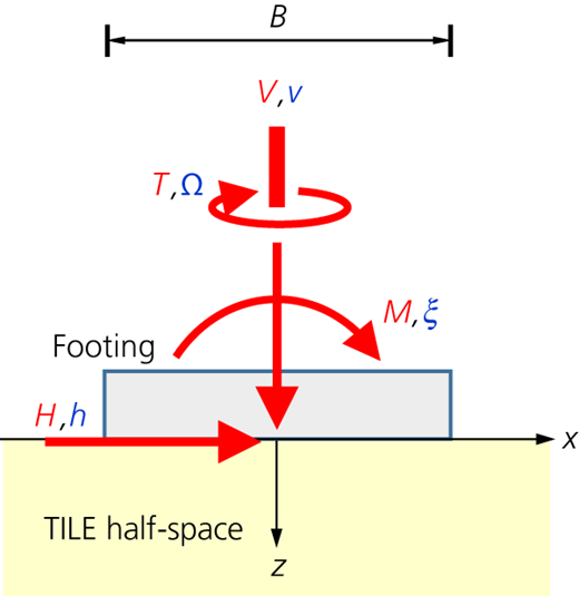
Generalised loads and conjugate displacements on a circular footing of diameter B on the surface of a uniform TILE half-space
Generalised loads and conjugate displacements on a circular footing of diameter B on the surface of a uniform TILE half-space
Present operative codes of practice including those by Det Norkse Veritas (DNV, 1992) and the International Organization for Standardization (ISO, 2016) quote formulae for footing stiffnesses that are based on an assumption of fully isotropic (FILE) soil behaviour. Table 1 lists some of these formulae. The case IDs are the shorthand used in the present paper. Some of the formulae make the further unrealistic assumption of frictionless contact between footing and soil. The aim of the present research was to develop formulae that take account of both transverse anisotropy and interface friction.
Stiffnesses of circular footings on FILE materials
| Symbol hereina | Case ID | Description | Equationb | By; notes |
|---|---|---|---|---|
| Kvv | VS | Vertical displacement, smooth interface | Boussinesq (1878); exact | |
| VR | Vertical displacement, rough interface | Spence (1968); exact | ||
| Khh | HR | Horizontal displacement, rough interface | Gerrard and Harrison (1970); approximatec | |
| Bycroft (1956), Poulos and Davis (1974); approximatec | ||||
| Gazetas and Tassoulas (1987); approximatec | ||||
| Kmm | MS | Overturning displacement, smooth interface | Borowicka (1943); exact | |
| MR | Overturning displacement, rough interface | (Graphical presentation) | Numerical results; Bell (1991)c | |
| Khm = Kmh | MR, HR | Rough interface | Up to 10% of direct stiffnesses (drained), 0 undrained | Numerical results; Bell (1991)c |
| Ktt | TR | Torsional displacement, rough interface | Reissner and Sagoci (1944); exact |
Superscript u may be used for undrained conditions
All equations assume full contact between the footing base and soil. μ = 0.5 for undrained conditions
Improved formulae are developed in this paper; see Equations 71–74
This research was made possible by the closed-form solutions by Liao and Wang (1998) for point loads on or in a TILE half-space. Gerrard and Wardle (1973) earlier proposed a solution for the special case of vertical loading. Anyaegbunam (2014) later proposed an equivalent formulation for this special case. Dean (2023) found that the solutions by Liao and Wang (1998) for general loading simplify greatly for the special case of surface loading, which is of interest in the present paper.
Starting points
Coordinates, notation and sign conventions
Figure 2 shows the coordinates used herein and the directions of positive change of stress. The origin is at the centre of the footing–soil interface, which is on the surface z = 0 of the TILE half-space. The z-axis is vertical and is the assumed direction of behavioural symmetry of the material. Both Cartesian (x, y, z) and cylindrical (r, θ, z) coordinates are used, and the lateral load H in Figure 1 is taken to be in the +x direction and resolved at the level z = 0.
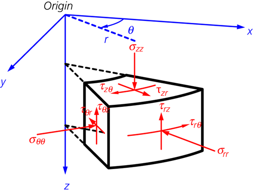
Cartesian and cylindrical coordinate frames and directions for positive stresses. The origin is at the centre of the soil–footing interface. The z-axis is vertical and is the axis of material symmetry. The surface of the half-space is at z = 0
Cartesian and cylindrical coordinate frames and directions for positive stresses. The origin is at the centre of the soil–footing interface. The z-axis is vertical and is the axis of material symmetry. The surface of the half-space is at z = 0
Symbols used herein for stress refer to changes in stress associated with elastic strains. Principal stresses and principal strains are taken positive in compression. For notational simplicity, the prime symbol is not used for effective stress. For example, σ rr represents a change of effective radial normal stress in a cylindrical r, θ, z coordinate frame. Following Lings (2001) and others, the superscript ‘u’ stands for total stress and for material constants for undrained behaviour.
Constitutive equations
The constitutive equations of TILE materials are well known, and the following development follows Gibson (1974) and Lings et al. (2000) with minor changes in notation. The relation between normal strains ϵ and changes in effective normal stress σ in general cylindrical coordinates with the axis of symmetry in the z-direction can be expressed as
E h and E v are non-negative normal moduli and are equal for an FILE material. Poisson’s ratios μ hh and μ vh are equal for an FILE material. Some authors, including Lings et al. (2000), use μ hv/E h instead of the equivalent μ vh/E v in the third row. However, the reciprocity relations by Onsager (1931) imply that the matrix is symmetric, and the present paper follows Gibson (1974) and others by incorporating the symmetry in the notation. The matrix determinant is Δ = Δ1Δ2/E v with
Δ1 ≥ 0 and Δ2 ≥ 0 are equivalent to limits deduced from strain energy considerations, discussed by Lings et al. (2000) and attributed to Love (1927), Raymond (1970) and Pickering (1970). For shear strains and changes in shear stress
The non-negative shear moduli G hh and G vh are equal for FILE materials. A combination of tensor rules and material symmetry about the z-axis gives
which reduces to a familiar relation for FILE materials (e.g. Davis and Selvadurai, 1996). For general TILE materials, there is no analogous relation for G vh.
Effective parameter values and ratios
Table 2 lists the sources of data of TILE material parameters explored in the present paper. These sources were selected from a much wider possible selection using the following criteria: (a) all five independent material constants of a TILE material should be given and (b) the experimental data should be tabulated so that actual values could be used. The data for the two sands were tabulated for different densities, applied stress magnitudes and radial-to-vertical stress ratios from 0.5 to 2. For the clays, data were mostly given for one or a small number of soil states for a given clay.
Data sources
| Source | Soil | Symbol in figures | Number of tests | Details |
|---|---|---|---|---|
| Sands | ||||
| Bellotti et al. (1996) | Ticino sand | ◆ | 26 | Their table 6 |
| Fioravante et al. (2013) | Carbonate Kenya sand | ● | 68 | Their tables 9 and 10 |
| Clays | ||||
| Lings et al. (2000) | Gault Clay | + | 1 | Their tables 1 and 3 |
| Jardine et al. (2004) | Bothkennar Clay | ⬛ | 1 | From Piriyakul (2006), table 2.5 |
| Piriyakul and Haegeman (2006) | Kaolinite clay | ⬛ | 1 | Their table 1 |
| Gasparre et al. (2007) | London Clay | ⬛ | 1 | Their table 4, HCA |
| Yimsiri and Soga (2011) | Gault Clay | ⬛ | 1 | Their table 2 |
| London Clay | ⬛ | 1 | ||
| Ratananikom et al. (2013) | Bangkok Clay | ⬛ | 1 | Their table 4 |
| Nishimura (2014) | Six natural clays | ⬛ | 10 | Nishimura’s table 1 |
| Six reconstituted clays | ⬜ | 6 | ||
| Brosse et al. (2017a; 2017b) | Four natural clays | ⬛ | 4 | Their table 4 |
| Nishimura and Magalona (2020) | Reconstituted kaolin clay | ⬜ | 1 | Their table 2 |
| Reconstituted Izumi clay | ⬜ | 2 | Their table 3 | |
HCA, hollow cylinder apparatus
Figures 3(a) and 3(b) show the relation between the effective normal modulus ratio E v/E h plotted horizontally against shear modulus ratio G vh/G hh for the soils of Table 2. Both ratios are 1 for FILE materials, so the spread of values, most less than 1, is an indication of the degree of anisotropy of these soils. For clays, Pegah et al. (2021) suggested a relation of the following form, based on the paper by Mašín and Rott (2014):
with a = 1 and b = 1.25. There is considerable scatter for the clays. The two sands show a similar but tighter relationship, with a = 1.1 and b = 2.5.
Figures 3(c) and 3(d) show values of Poisson’s ratios μ hh and μ vh, also plotted against the effective normal modulus ratio. The sands have μ hh about equal to 0.2, not strongly dependent on the density or stress or modulus ratio. For the clays, both positive and negative μ hh values are seen, but almost all had positive values of μ vh. Some authors have reported considerable difficulty in measuring this parameter for clays, partly due to strain dependence.
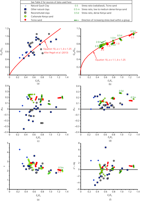
Aspects of the transverse anisotropy of some geomaterials, drained parameters: (a) modulus ratios for clays, (b) modulus ratios for sands, (c, d) Poisson’s ratios, (e, f) Liao and Wang (1998) dimensionless parameters s and s 2 − 4q
Aspects of the transverse anisotropy of some geomaterials, drained parameters: (a) modulus ratios for clays, (b) modulus ratios for sands, (c, d) Poisson’s ratios, (e, f) Liao and Wang (1998) dimensionless parameters s and s 2 − 4q
Liao and Wang (1998) parameters
The equations by Liao and Wang (1998) for displacements and changes of stress due to point loads are written in terms of the constrained moduli A ij, with
with A 12 = A 11 − 2A 66. The shear moduli are A 44 = A 55 = G vh and A 66 = G hh, and all other A ij are zero. Inverting Equation 3 gives
Expressions for the constrained moduli in Equation 11 can be obtained by direct comparison with this.
The point load solutions by Liao and Wang (1998) use adjusted vertical coordinates z i = u i z, where u i are dimensionless factors. The factors are 1 for FILE materials but differ from 1 for TILE materials, indicating that stress, strain and displacement are transmitted a little differently through a TILE body. The factors satisfy the following equations:
The first is the ‘characteristic equation’ for TILE materials. It serves to define the dimensionless variables m 1 and m 2, with the equality between the two expressions for m i arising from equilibrium equations. By expanding this equality, Liao and Wang (1998) showed that the dimensionless variables u 1 and u 2 satisfy a quadratic , with
If s 2 < 4q, then and are complex conjugates. The present paper takes the upper sign for i = 1 and the lower for i = 2. The formulae by Liao and Wang (1998) for s and q imply
Liao and Wang (1998) considered three solution cases, depending on the sign of s 2 − 4q. Dean (2023) confirmed that u i are either both real or are complex conjugates of each other. The latter feature does not lead to complex results for measurable engineering quantities because, as shown later in this paper, such quantities are the sums of components in which the imaginary parts cancel. This is consistent with Anyaegbunam (2014), who showed that the results for vertical loading can be rewritten in a way that avoids explicit use of complex variables.
Using the first equality in the characteristic equation, one can readily show that m 1 m 2 = u 1 u 2. This is found to produce major simplifications when the results by Liao and Wang (1998) are applied for a point load at the surface of the half-space. Dean (2023) introduced the following variables based on results by Liao and Wang (1998):
These are dimensionless constants and are infinite in the special case when s 4 = 4q. Indeed, this is the case for the special case of a fully isotropic (FILE) material, but it is found that cancellations then apply so as not to produce infinite results for displacements, strains or stresses.
Parameters for soils
Figure 3(e) shows that s is positive for the data of Table 2 and in most cases greater than 2. Figure 3(f) shows that s 4 = 4q can be positive or negative for these soils. As noted earlier, u 1 and u 2 are complex conjugates when this is negative, while the displacements, strains and stresses in the material remain real. The results for the sands show that the parameter can vary depending on stress, stress ratio and density. It will be seen later that the change from positive to negative values does not produce any problem in the measurable stiffnesses calculated for the circular footing.
Point load equations
Figure 4 shows a local coordinate geometry for calculations for displacements due to point loads P z vertically and P x horizontally applied to the half-space. The origin is at the load point and is called P. The direction of the load P x defines a local x-axis, and θ PA is the azimuthal angle in the z = constant plane from this axis to a point of interest.
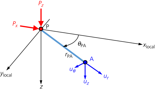
Local geometry for point load calculations. The origin is at the load point. The local x-axis is in the direction of the applied lateral load. The soil surface is z = 0
Local geometry for point load calculations. The origin is at the load point. The local x-axis is in the direction of the applied lateral load. The soil surface is z = 0
Table 3 gives the displacements in the material body due to the point loads P x and P z. The solutions for the TILE material have been calculated from the results by Liao and Wang (1998), taking their symbol P r to represent the force in the +x direction. Detailed checks by Dean (2023) confirm that this gives equations that have correct symmetries and for which compatibility, material behaviour and equilibrium are all satisfied. The geometric parameters are as follows:
For the TILE half-space, the equations for displacements under vertical point load involve parameters and . The equations for the TILE material reduce to those for the FILE material when the material constants are those of an FILE material.
Radial, circumferential and vertical displacements of the material of the half-space
| FILE half-space | TILE half-space | |
|---|---|---|
| Vertical point load Pz | ||
| Uθ = 0 | Uθ = 0 | |
| Boussinesq (1875) | Liao and Wang (1998), interpreted by Dean (2023) | |
| Horizontal (+x) point load Px | ||
| Cerruti (1882–1885) | Liao and Wang (1998), interpreted by Dean (2023) | |
| See also | Westergaard (1952), Davis and Selvadurai (1996), Podio-Guidugli and Favata (2014) | Gerrard and Wardle (1973), Anyaegbunam (2014). Note: in formulae for vertical load |
Inspection of Table 3 reveals that the consequent material displacements (u r, u θ, u z) at a point A on the surface at coordinates (r, θ, z) = (r PA, θ PA, 0) are given by equations of the following form:
The dimensionless ‘compliance factors’ C ab are listed in (a) in Table 4. The expressions for an undrained material are identified by superscript u and are obtained by applying the equations for the drained case but using the equations of Gibson (1974) for and , as detailed by Dean (2023).
Compliance factors
| (a) Basic factors | ||||
|---|---|---|---|---|
| Factora | Description | FILE material | TILE material | |
| Drained | Undrained | |||
| Czz | Vertical displacement due to vertical force | 1 − μ | ||
| Czx | Vertical displacement due to horizontal force | 0 | ||
| Crz | Radial displacement due to vertical force | 0 | ||
| Crx | Radial displacement due to horizontal force | 1 | ||
| Cθz | Circumferential displacement due to vertical force | 0 | 0 | 0 |
| Cθx | Circumferential displacement due to horizontal force | μ − 1 | ||
| (b) Composites | ||||
| Factor | Description | Definition | FILE material | |
| C 2 | Circumferential–radial coupling factor | |||
| C 4 | Vertical–radial coupling factor | |||
| C 5 | Horizontal–vertical coupling factor | |||
The superscript u may be used for undrained conditions. Formulae for undrained compliance factors are obtained by using undrained material parameters in the formulae for drained conditions
Point load compliance factors for soils
Figure 5(a) shows C zz plotted against normal effective modulus ratio E v/E h. The value for an FILE material is 1 − μ, which varies between 1 and 0.5 for μ in the typical range 0–0.5. The high values of C zz for clays at low E v/E h would correspond to negative values of an equivalent μ.
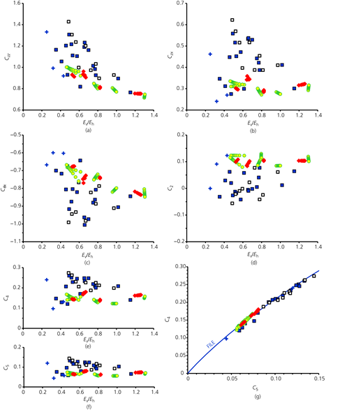
Compliance factors plotted against (a–f) modulus ratio and (g) each other. See Table 2 for data sources and key
Compliance factors plotted against (a–f) modulus ratio and (g) each other. See Table 2 for data sources and key
Figure 5(b) shows that C zx is approximately 0.3 for the two sands. The value for an FILE material is 0.5 − μ, so the 0.3 would correspond to an equivalent μ of 0.2. Some of the higher values for the clays would give a negative equivalent μ. The square of C rx is plotted in Figures 3(a) and 3(b). Figure 5(c) shows that C θx is mostly in the range −0.6 to −1. The value for an FILE material is μ − 1, which is in a similar range for μ in the typical range 0–0.5.
Figures 5(d)–5(f) show the three composite parameters defined in (b) in Table 4. Each has a low spread – for example, C 5 is mostly between 0.05 and 0.15. Figure 5(f) shows that C 4 and C 5 are closely related and that the TILE data of Table 2 follow closely the curve calculated for FILE materials.
Figure 3(f) shows that the sign of s 2 − 4q can depend on test conditions. The plots in Figure 5 confirm that this does not cause any discontinuity in the variation of compliance factors. Discontinuities in algebra do occur when the sign changes, but they occur with opposite signs in the two components of the expressions in (a) in Table 4 and so cancel each other.
Displacement calculations at the footing–soil interface
Figure 6 shows a plan view of the geometry used to calculate displacements of soil on the circular footing–soil interface due to stresses on this interface. One-quarter of the interface is shown. The global Cartesian coordinate axes x, y are on the surface of the TILE half-space, and the z-direction is downwards, into the paper. The global coordinate origin O is at the centre of the interface. Angles in the xy plane are measured clockwise in this plan view.
Plan view of one-quarter of the bearing area and global coordinate system (x, y) for calculating the effects of interface stresses at P on the displacements at A
Plan view of one-quarter of the bearing area and global coordinate system (x, y) for calculating the effects of interface stresses at P on the displacements at A
Point P represents a load point, with global radial and azimuthal coordinates r and θ. An infinitesimal area da of the interface around P supports loads that are products of da with the interface stresses σzz vertically, τzr radially in direction OP and circumferentially τzθ in the direction at 90° clockwise from OP:
These are considered point loads in the limit as da → 0.
Displacements at some other point A are of interest. This point has radial and azimuthal coordinates rA and θA, and it is convenient to define an adjusted azimuth φ = θ − θA (which is negative for points P and A as drawn in Figure 6). For a given point A, integrals over the area of the soil interface can be carried out with either da = rdrdθ or da = rdrdφ. The distance from P to A is rPA, with
The net displacement at a given point A will be calculated by integrating for all infinitesimal areas around points PA on the soil–footing interface. When doing this integral, it will be equally valid to take da = rdrdθ and take the angular part of the integral to go from θ = 0 to 2π radians or to take da = rdrdφ with angles from φ = 0 to 2π radians.
It is convenient to set up two local Cartesian coordinate frames centred on P. One has its local x-axis in the direction of the load dPx1, the second has its local x-axis in the direction of dPx2. The correspondence between Figures 4 and 6 is different for the two loads, as follows. For the first load, dPx1, the angle θPA in Figure 4 becomes χ − θ in Figure 6, where χ satisfies
where cx and sx are convenient abbreviations. Using standard trigonometric formulae and making two further convenient abbreviations gives
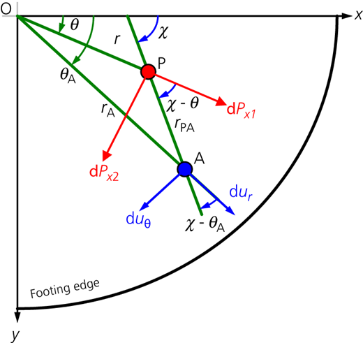
For the second load, dPx2, the local x-axis points in the direction at 90° clockwise from OP. The angle θPA in Figure 4 becomes χ − θ − 90° in Figure 6. With respect to P, the displacements at point A in either of the local coordinate frames are as follows:
where ‘radial’ means the direction from P to A and ‘circumferential’ at 90° clockwise from PA. To obtain the displacements in the global cylindrical coordinate frame, it is necessary to resolve in the radial and circumferential directions relative to point O. This involves the angle χ − θA, which satisfies
where cA and sA are convenient abbreviations. Resolving gives, in the global coordinates
The net displacements of the soil at point A on the interface are obtained by integrating over all the infinitesimal areas of the footing–soil interface.
Results are given in (a) in Table 5. The equations are general and can be used for calculations for flexible footings, rigid footings and heaps and for an interface of any shape. The equations can be rewritten in terms of Cartesian coordinates using the following procedure.
To convert the equations in (a) in Table 5 to give displacements in Cartesian coordinates, change (r, θ) to (x, y) on the left of the equations and change subscript A to subscript χ on the right.
To convert the equations in (a) in Table 5 to use stresses in Cartesian coordinates, change (r, θ) to (x, y) in the stress subscripts on the right, and change subscript P to subscript χ on the right.
Soil displacements on the soil–footing interface assuming full contact is maintained
| (a) General equations, for vertical, radial and circumferential directions respectively | ||
|---|---|---|
| (b) Normalised equations, cases MR and HR, for vertical, radial and circumferential directions respectively | ||
| (c) Re-stated equations, cases MR and HR, for vertical, lateral difference and lateral sum respectively | ||
The subscripts on the compliance factors do not change. For both displacements and stresses in Cartesian coordinates, both actions are needed. (b) and (c) in Table 5 give some further adaptations, which are described later in this paper.
Closed-form solutions for TILE materials
Overview
Four closed-form solutions for stiffness and interface stress are developed in this section. The method for the first three is to start with a known solution for FILE materials, find out where the single relevant compliance factor is for these and then replace it with the factor for TILE materials. Table 6 gives key equations for the first three. In the following text, parts of the table are referenced as ‘cells’ with a letter identifying the column and a number the for row.
Development of simple closed-form solutions: from FILE to TILE half-spaces
| Item | (A) Case VS: vertical displacement v on a smooth interface | (B) Case TR: torsional displacement BΦ on a rough interface | (C) Case MS: overturning displacement Bξ on a smooth interface |
|---|---|---|---|
| (1) Displacement equation to be soved | |||
| (2) Normalised stress | |||
| (3) Normalised equation to be solved | |||
| (4) Solution for stress | After Boussinesq (1875) | After Reissner and Sagoci (1944) | After Borowicka (1943) |
| (5) Force resultant | |||
| (6) Solution for normalised stress | |||
| (7) Stiffness |
Case VS: vertical load and smooth interface
In this case, the change σ zz of vertical stress is the only non-zero change of interface stress. The radial and circumferential displacements are uncontrolled. The vertical displacement at all points in the soil on the interface is some value u z = v, and the equation for this in (a) in Table 5 reduces to the equation in cell A1 of Table 6. One can immediately guess, correctly, that the vertical stiffness is obtained by replacing 1 − μ with C zz in the equation for this case in Table 1.
To check this, it proves useful to define a normalised, dimensionless stress S z by the equation in cell A2 of Table 6, where r′ = 2r/B is a normalised radius with a value of 0 at the centre and 1 at the edge of the soil–footing interface. The displacement equation then reduces to that in cell A3, where da′ = 4da/B 2 is a normalised area.
The normalised equation does not contain any information on whether the material is an FILE or a TILE one. It applies for both. Therefore, it is satisfied by the solution of Boussinesq (1875) for an FILE material. His solution for stress is in cell A4, with the vertical force V resultant in cell A5. Using these in the previous equations to calculate S z gives the result in cell A6. Putting this into the stress equation in cell A2 and calculating the force resultant and then V/v gives the stiffness in cell A7.
Case TR: torsional displacement and rough soil–footing interface
Reissner (1937) and Reissner and Sagoci (1944) show, by symmetry, that the only non-zero interface stress in this displacement case is the circumferential shear stress. The circumferential displacement is u θ = rΦ, where Φ is the angle of rotation about the vertical axis through the centre of the footing. The equation for circumferential displacements in (a) in Table 5 reduces to the following:
where the shear stress τ zθ is independent of azimuth. Using Equations 32, 35 and 40
where the partial differential is at constant r A and r. It follows that, since τ zθ is independent of azimuth, the integral with c P c A in the previous equation is zero. Hence, −C θx c P c A can be replaced with C rx c P c A without changing the result of the integration. Using a standard trigonometric formula implies c P c A + s P s A = cos φ. This leads to the revised displacement equation in cell B1 of Table 6.
Cell B2 gives a suitable definition for normalised stress S θ for this case. The displacement equation then reduces to that in cell B3. The closed-form solution by Reissner and Sagoci (1944) for an FILE half-space is given in cell B4. The force resultant T/B is given in cell B5. Using these in the previous equations reveals the result for S θ in cell B6. Using this in cell B2 and carrying out the integration in cell B5 then produces the stiffness in cell B7.
The Appendix shows that for this special case, the changes in stresses within the TILE material can be found in closed form.
Case MS: overturning displacement and smooth soil–footing interface
Borowicka (1943) proposed a solution for this case. The smooth interface implies that the only interface stress that changes is the vertical stress. For calculation herein, it is assumed that the interface can take a negative values of the change of this stress due to moment, so that there is no loss of contact between the soil and any part of the footing. This can be so if there is sufficient simultaneous vertical load.
If the footing rotates through ξ about the global y-axis, the displacement at location (r A, θ A) on the soil–footing interface is u z = r A ξcos θ A. With no interface friction there can be shear loads, and the displacement equation for vertical displacement in (a) in Table 5 reduces to that in cell C1 of Table 6. The symmetry of this displacement suggests that the stress will have the same symmetries as cos θ. To explore this, it proves useful to define a normalised stress S z as in cell C2. Substituting this into cell C1 and converting to normalised parameters gives
Using the identity cos θ = cos φcos θ A − sin φsin θ A gives
The second integral over the azimuthal coordinate is zero if S z is a function solely of radius. This is because sin φ makes the integrand odd in φ. The cos θ A factors can then be cancelled from both sides of the result, giving the normalised displacement equation in cell C3.
The equation has the same form as in cell B3, so a solution can indeed be found, with the value of S z given in cell C6, independent of azimuth. The stiffness in cell C7 follows by substituting this in the equation in cell C2 and integrating according to cell C5. This result, which is for a general TILE material with its compliance factor C zz, is found to be consistent with the solution by Borowicka (1943) for an FILE material in Table 1, with its factor C zz = 1 − μ.
Case VR: vertical displacement and rough interface
This case is similar to case VS except that the radial interface shear stress can develop to prevent radial displacements of the soil on the interface relative to the footing. The method of analysis is broadly the same as for the simpler case VS, but with some extra complications.
Symmetry implies that the changes in vertical and radial interface stresses are independent of azimuth and that no changes in circumferential stress will occur as a result of the imposed downward vertical displacement v. Equations for the vertical and radial displacement will be relevant, and the independence of azimuth means that −C θx c P c A can be replaced with C rx c P c A, such as in cases TR and MS. This results in the following displacement equations:
It is found convenient to define three dimensionless stresses as follows, where the first is the same as for case VS:
Both S r and will be useful. The displacement equations in Equations 49 and 50 then give
with C 4 as defined in (b) in Table 4. Equations 54 and 55 do not contain any explicit information about whether the material is an FILE or a TILE one. They therefore apply for both. They contain only one controlling variable, C 4. Hence, the solutions for the normalised stresses S r and can depend only on C 4. It then follows from the equation for vertical stress and from the force resultant integral in cell A5 in Table 6 that the vertical stiffness will have the following form:
where K′(C 4) is a function only of C 4. The value of C 4 for an FILE material is given in (b) in Table 4. Solving for Poisson’s ratio gives
Using this in the exact solution by Spence (1968) for K vv for a rough interface in Table 1, and comparing the result with Equation 56, gives
One might call S(ψ) ‘Spence’s function’, since it comes ultimately from the exact analysis by Spence (1968). Figure 7(a) shows the variation of S(ψ) with ψ. Its value is 2 at ψ = 0 and rises at first slowly with increasing ψ. It reaches infinity at ψ = 1. Figure 7(b) shows variations of C n and S(C n) − 2 with μ for FILE materials. Figures 7(c) and 7(d) show values of S(C 4) and S(C 5) for the TILE samples of Table 2.
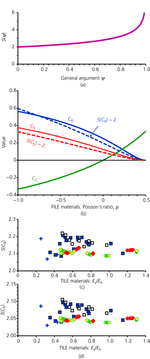
Spence’s function and applications. See Table 2 for data sources and key and Equation 58 and Table 4 for definitions
Cases MR and HR: preliminary calculations
Normalisations
Cases MR (overturning displacement, rough interface) and HR (horizontal +x displacement, rough interface) involve all three types of interface stress. It will be convenient to consider them together. The actual displacements at a point (r A, θ A) on the soil–footing interface are listed in (a1) in Table 7, where ξ is the overturning angle and h is the horizontal displacement.
Cases MR and HR, drained condition
| (a) Definitions for (b) in Table 5 | |||
|---|---|---|---|
| Vertical | Radial | Circumferential | |
| (1) Actual displacements | uz = rAξ cos θ A | ur = h cos θ A | uθ = −h sin θ A |
| (2) Normalised stresses | |||
| (3) Normalised displacements | |||
| (b) Definitions for (c) in Table 5 | |||
| (1) Composite normalised stresses | |||
| (2) Cosines | |||
| (c) Approximate solutions | |||
| Case MR, k = Bξ/2 | Case HR, k = h | ||
| (1) Definition | |||
| (2) Actual stiffnesses | |||
| (3) Normalised stiffnesses | |||
In the simpler case MS considered earlier, an assumption was made regarding the azimuthal variation of vertical stress, and this simplified the displacement equation and was found to give a correct closed-form solution. In cases MR and HR, the following analysis assumes that the stresses vary with θ just as the actual displacements vary with θ A. It is then useful to define normalised stresses S z, S r and S θ as in (a2) in Table 7, where k = Bξ/2 for case MR and k = h for case HR.
When these are substituted into the displacement equations in (a) in Table 5, it becomes possible to identify integral parts that are zero because the integrals are odd functions of φ. It is then found convenient to define normalised displacements as in (a3) in Table 7. Their values are for case MR and (0, 1, −1) for case HR. Trigonometric factors involving θ A can then be cancelled as in case MS, leaving the normalised equations of (b) in Table 5.
In both cases MR and HR, moments M will develop as a result of the displacement k. Integrating the vertical stress in (a2) in Table 7 appropriately gives
The interface shear stresses τ zx and τ zx in the x- and y-directions are obtained from the normalised stresses in (a2) in Table 7 as follows:
Integrating the first over the interface, and assuming that the normalised radial and circumferential shear stresses are independent of azimuth, gives the horizontal load in the +x direction:
Integrating the shear stress in the y-direction gives zero because is an odd function of θ.
Approximate solutions for the drained condition
Numerical results presented later will show that S y is typically small compared with S x for cases MR and HR. The following approximate analyses are possible if S y is ignored completely and will later be checked numerically.
The first is for case MR, for which and . It is convenient to define a new normalised stress associated with the x-direction as in (c1) in Table 7. With S y = 0, the first two equations in (c) in Table 5 then give
with C 5 as given in (b) in Table 4. C 5 is the only independently controllable parameter in these equations. Hence, the solutions for normalised stresses will be functions of C 5. (a2) in Table 7 shows that the stresses also involve C zz. On this basis and using Equations 60 and 63, approximate stiffnesses for case MR will have the forms in (c2) in Table 7, with the normalised stiffnesses of (c3) in Table 7 being functions of C 5.
The second approximate analysis is for case HR, for which and . It is convenient to define two new normalised stresses as in (c1) in Table 7 for case HR. With S y = 0, the first two equations in (c) in Table 5 then give
C 5 is the only independently controllable parameter, so the solutions for the new normalised stresses will be functions of C 5. (a2) in Table 7 shows that the stresses also involve C zz. On this basis and using Equations 63 and 60 and with k = h, approximate stiffnesses for case HR will have the forms in (c2) in Table 7, with the normalised stiffnesses of (c3) in Table 7 being functions of C 5.
The reciprocity relations by Onsager (1931) imply that the stiffness matrix in Equation 2, which relates conjugate quantities, should be symmetric, so that K hm = K mh. Hence, using (c2) in Table 7:
From Table 4, C rz = −C zx. Hence
This is confirmed numerically later by testing whether K hm, calculated for case MR, equals K mh, calculated for case HR.
Numerical implementation
Aims and method
Numerical analyses were carried out to check the algebra presented earlier and to analyse cases for which closed-form solutions were not found in the literature. Bespoke software for this research was written in Microsoft Excel VBA. The linearity of the FILE and TILE behaviours makes the boundary-element method possible for this. The method is well established and described by Brebbia (1978), Banerjee and Butterfield (1981), Katsikadelis (1982, 2016), Zhou et al. (2019) and others.
Boundary discretisation
Figure 8 shows the key features of the discretisation used in the present study. Only one-half of the interface was used explicitly, with the other half being represented through symmetry of refection in the x-axis.
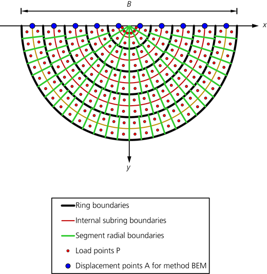
The interface was discretised into a number N R of concentric, equally spaced rings. The central ring had an inner normalised radius 0, and so it formed a circle of normalised diameter 2/N R about the centre of the footing. Each ring was discretised into a number N S of equally spaced subrings. A given discretisation is thus characterised as an N R/N s one. The mesh in Figure 8 is 5/2, while 100/10 meshes were used in the present calculations. Each subring was discretised in the azimuthal direction into a number of segments. Except at the centre, the number was calculated to make all segments approximately curvilinear squares. As a result, except for the innermost ring, most segments were close to the same size. A 100/10 mesh contained about 1.57 million segments.
Methods
Displacements on the interface due to stress on a segment were calculated assuming that they would be the same as displacements due to a point load at a representative point at the plan centroid of the segment. This was not accurate for points close to a given segment, but the overall effect of this inaccuracy was minimised by using a fine mesh. Normalised stresses at nodes on φ = 0 were the ultimate unknowns, with expected variations with azimuth incorporated into the calculations. Displacements at points A on φ = 0 were the givens for any given footing displacement condition.
In one calculation option, labelled ‘BEM’, matrix relations between nodal displacements and nodal normalised stresses were calculated and the relevant system of vector and matrix equations were solved. This was found to be subject to spurious end effects, at both r′ = 0 and r′ = 1, but effects on calculated stiffnesses were negligible for meshes finer than about 20/5. In a second option, labelled ‘LSQ’, a given normalised stress S was assumed to be given by a sum of functions f i weighted by scalar factors w i:
The weights were found by minimising the variances between calculated displacements and the displacements imposed by the rigid footing. The available functions were mostly of the form r′m/(1 − r′2)1/2. Fewer than ten functions were needed to achieve consistency with the BEM method. End effects were handled better, but the set of functions did not have the same type of linear independence as occurs in Fourier analysis, making interpretation more difficult.
For a 100/10 mesh, a typical calculation time on a middle range laptop was around 1 min for case VS and 6 min for cases MR and HR.
Numerical results
Results for FILE materials
Figure 9 shows results for FILE materials. On the left, the calculated stiffnesses are for full interface friction and are plotted in dimensionless forms K/(GB) against Poisson’s ratio. The filled circles are for the VBA calculations of the present project and are in general agreement with the finite-element results of Bell (1991) represented by the + symbols. Also shown are curves, which represent proposals by previous authors. The solution by Spence (1968) in Figure 9(a) is exact for a frictional interface. The solutions by Boussinesq (1878) and Borowicka (1943) are exact for a frictionless one. The solutions by Bycroft (1956), Gerrard and Harrison (1970) and Gazetas and Tassoulas (1987) are from approximate analyses.
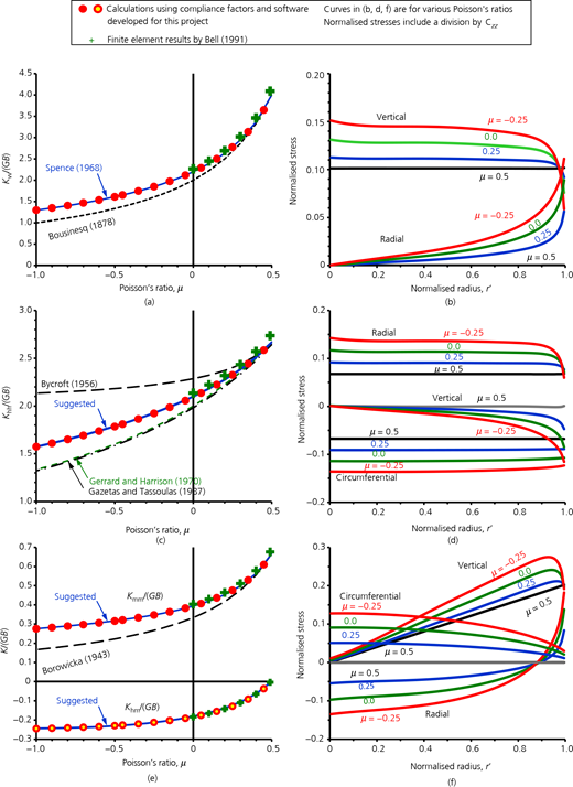
Effects of friction and Poisson’s ratio for FILE materials and fully rough soil–footing interface: (a, b) case VR, vertical displacement (and comparison with VS); (c, d) case HR, horizontal displacement; (e, f) case MR, overturning (and comparison with MS)
Effects of friction and Poisson’s ratio for FILE materials and fully rough soil–footing interface: (a, b) case VR, vertical displacement (and comparison with VS); (c, d) case HR, horizontal displacement; (e, f) case MR, overturning (and comparison with MS)
On the right, the curves of normalised stresses have been calculated by using the numerical software. The normalised stresses are plotted against normalised radius for various values of Poisson’s ratio. The results give a visual impression of the effects of different values of Poisson’s ratio. Note, however, that the normalised stresses (Table 6) include C zz in their denominators, and in some cases the ordering of the curves is different from that for the actual stresses.
In Figure 9(a), the numerically calculated results for case VR agree with the exact solution of Spence (1968) over the full range of possible Poisson’s ratios. The solution of Boussinesq (1875) for a frictionless interface (case VS) gives the same vertical stiffness if μ = 0.5. This is because the compliance factors C zx and C rx are zero when μ = 0.5, giving no coupling between vertical and lateral directions. The solution of Boussinesq (1875) gives a stiffness at μ = 0 about 10% lower than that for a frictional interface.
Figure 9(b) shows the numerically calculated changes of normalised vertical and radial stresses for case VR. For μ = 0.5, the value is constant with radius and is 1/π 2, consistent with cell A6 in Table 6. At lower values of μ, the results are consistent with a normalised vertical stress of zero at the edge of the footing. The normalised radial stress is non-zero, so the actual radial stresses are infinite there. A breakdown of linearity at the edge is well known since real materials cannot sustain the infinite vertical stress predicted by the solution of Boussinesq (1875). However, the present results suggest that, with friction, the breakdown may be driven by interface friction rather than by vertical stress.
In Figure 9(c), numerically calculated results for case HR are shown to be consistent with the finite-element results of Bell (1991) and different from the approximate equations proposed by Bycroft (1956), Gerrard and Harrison (1970) and Gazetas and Tassoulas (1987). The suggested curve is
where S(…) is Spence’s function (Equation 59). The form of the right side was suggested by the form of the approximate solution in (c) in Table 7, and the constants 2.2 and 0.4 were obtained as an empirical fit to the numerical results.
Figure 9(d) shows numerically calculated changes in normalised stresses for case HR. For each of the four μ values, S θ = −S r at the centre of the footing. This ensures that the shear stress τ zx in the x-direction is continuous in the neighbourhood of the centre. For μ = 0.5, the normalised vertical stress is zero because the compliance factor produces no vertical–lateral coupling at this value, and the normalised radial and circumferential stresses are constant with radius. At lower values of μ, the compliance factors produce a coupling effect that causes vertical stresses to develop.
In Figure 9(e), numerically calculated results for case MR are seen to be consistent with the finite-element results of Bell (1991). The dimensionless moment stiffness is the same as that by Borowicka (1943) at μ = 0.5 and about 20% larger at μ = 0. The calculated coupled stiffness at given μ was found to be equal to that calculated from case HR to within 2%. The suggested curves are
where S(…) is Spence’s function (Equation 59). The forms on the right side were suggested by the forms in (c) in Table 7, and the constants were obtained as empirical fits to the numerical results.
Figure 9(f) shows numerically calculated normalised stresses for case MR. The result for μ = 0.5 is that same as for the solution of Borowicka (1943), with a linear variation for the vertical component and zero for the radial and circumferential normalised stresses. In all cases, S r + S θ = 0 at the centre of the footing. This is consistent with the requirement for shear stress to be continuous there. Curves for the radial components have a slight slope, which is a spurious end effect. Its effect on stiffness is considered to be negligible because the main contributions to stiffness come from larger radii.
The changes of radial stresses in Figure 9(f) change sign at about r′ = 0.9. This is interpreted as a result of a competition between competing effects. Without friction, the positive changes in vertical stresses would induce outwards soil movements. The negative components of change of radial shear stress resist this, and so maintain no net radial movement. In contrast, the effect at large enough radii would be to push the soil inwards, and positive change in shear stress develops to prevent this movement.
Results for TILE materials
Figure 10 shows numerical results for the TILE materials of Table 2, represented by points, together with curves, which represent theoretical expressions of empirical fits. Dimensionless stiffnesses are plotted on the left against 1 − C zz. From Table 4, one might interpret this as an equivalent isotropic Poisson’s ratio. Stress distributions for TILE materials did not reveal any significant new information. Instead, the plots on the right show the results in ways determined by expected functional forms.
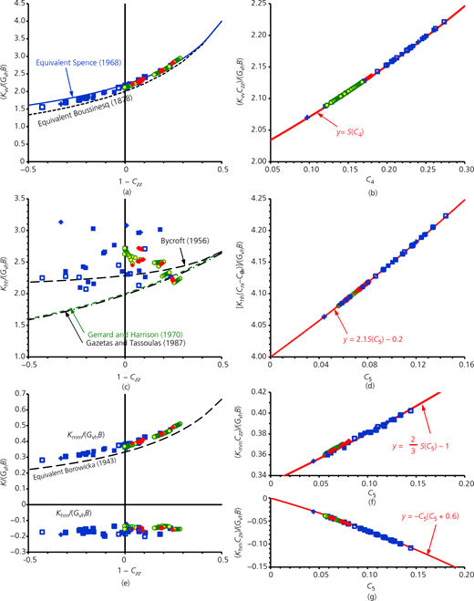
Effects of friction and anisotropy: TILE materials and fully rough soil–footing interface: (a, b) vertical displacement; (c, d) horizontal displacement; (e–g) overturning. See Table 2 for data sources and key
Effects of friction and anisotropy: TILE materials and fully rough soil–footing interface: (a, b) vertical displacement; (c, d) horizontal displacement; (e–g) overturning. See Table 2 for data sources and key
In Figure 10(a), the numerical results are for case VR. The two curves are calculated from the formulae for FILE materials by Spence (1968) and Boussinesq (1878) taking μ = 1 − C zz. They enclose most of the results, and either would certainly be sufficiently accurate for most practical engineering applications. In Figure 10(b), the aim is to check whether the exact solution of Equation 58 applies. The results confirm that it does.
In Figure 10(c), for case HR, the theoretical curves are calculated using μ = 1 − C zz in the formulae for FILE materials by Bycroft (1956), Gerrard and Harrison (1970) and Gazetas and Tassoulas (1987). The numerical results suggest that these formulae may be less useful for TILE materials. In Figure 10(d), the aim is to explore whether the approximate solution of (c) in Table 7 applies and to find the form of if so. The results indicate that it does apply and that the formula is
This is a surprisingly good fit to the numerical results. It appears to be slightly inconsistent with the corresponding Equation 71 for FILE materials, but the difference is small enough to be neglected for many practical engineering applications.
In Figure 10(e), for case MR, the theoretical curve calculated using μ = 1 − C zz in the formula of Borowicka (1943) gives a lower bound to stiffnesses. In Figures 10(f) and 10(g), the aim is to explore whether the approximate solutions of (c) in Table 7 apply and to find the forms of the formulae if so. The results are closely consistent with Equations 72 and 73.
Further considerations
Summary for the drained condition
Table 8 gives a summary of the results obtained for TILE materials in the drained condition. For cases VS, VR, MS and TR, the solutions are exact. For cases HR and MR, the solutions are fit to the results of the boundary-element calculations.
Stiffnesses of circular footings on TILE materials
| Symbol herein | Case ID | Description | Equationa , b | By; notes |
|---|---|---|---|---|
| K vv | VS | Vertical displacement, smooth interface | Adapted from Boussinesq (1878); exact, (a) in Table 5 | |
| VR | Vertical displacement, rough interface | Adapted from Spence (1968); exact, Equation 58 | ||
| K hh | HR | Horizontal displacement, rough interface | Fits to numerical results:
| |
| K mm | MS | Overturning displacement, smooth interface | Adapted from Borowicka (1943); exact, (c) in Table 5 | |
| MR | Overturning displacement, rough interface | Fit to numerical results, Equation 72 and Figure 10(f) | ||
| K hm = K mh | MR, HR | Lateral-moment coupling, rough interface | Fit to numerical results, Equation 73 and Figure 10(g) | |
| K tt | TR | Torsional displacement, rough interface | Adapted from Reissner and Sagoci (1944); exact, (b) in Table 5 |
Assuming full contact between footing base and soil
S(Cn) involves Spence’s function S, Equation 59
These results generalise those of Table 1, and the exact solutions are exactly equivalent to those in Table 1 when the compliance factors are chosen for FILE materials. For cases HR and MR, the solutions of Table 8 are also valid when FILE factors are used and give a better fit to the boundary-element calculations than the previous proposals included in Table 1.
Table 8 is also valid for the undrained condition, provided that the relevant undrained compliance factors are used. This condition is explored in more detail in the following.
Undrained condition
For an FILE material, the undrained condition is modelled with μ = 0.5 (e.g. Davis and Selvadurai, 1996). This gives for the FILE material (Table 4), so the equations in Table 5 produce no coupling between vertical and lateral directions. The interface therefore acts as if frictionless for cases VS, VR, MS and MR, and these cases are solved using (A) and (C) in Table 6 with the undrained . For cases VS and MS, the stiffness ratios satisfy
Figure 11(a) shows for the TILE materials of Table 2, and Figure 11(b) shows the ratio . This is less than 1 in all cases, implying that the undrained vertical stiffness is greater than the drained stiffness for case VS. Figure 11(c) shows the ratio of calculated vertical stiffnesses including the effects of friction in the drained case, and Figure 11(d) shows the ratio for calculated horizontal stiffness. The analogous ratio for moment stiffness is not shown in the figure, but it was found to be almost identical to that for vertical stiffness. In all cases, the undrained stiffness is greater than the drained stiffness.
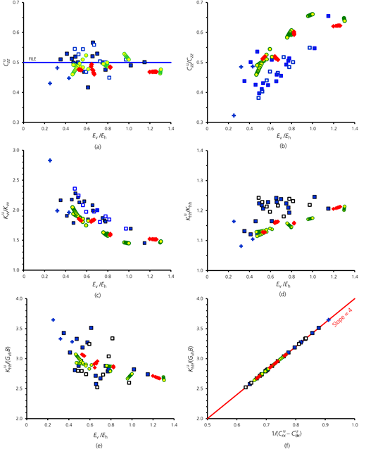
Undrained results for TILE materials: (a) compliance factor C zz, (b) ratio of undrained to drained compliance factors, (c,d) ratios of undrained to drained stiffnesses, (e,f) normalised horizontal stiffnesses. See Table 2 for data sources and key
Undrained results for TILE materials: (a) compliance factor C zz, (b) ratio of undrained to drained compliance factors, (c,d) ratios of undrained to drained stiffnesses, (e,f) normalised horizontal stiffnesses. See Table 2 for data sources and key
Torsional stiffness is independent of drainage conditions because it is determined by the shear moduli ((B) in Table 6). Compliances are not involved.
For case HR, the numerical results in Figure 9(d) for μ = 0.5 show radial and circumferential normalised stresses, which were the negatives of each other. This was also seen in calculations for undrained responses. With , equations in Table 5 imply that no vertical displacements are induced by interface shear stresses. Consequently, no vertical stress develops, and the last two equations in (c) in Table 5 give for the undrained case
A bespoke program was developed in Microsoft Excel VBA to investigate these equations. It was found that if is constant with radius, the first integral in the second equation is zero for all nodal points within the interface:
An advanced online symbolic algebra program found this integral too difficult, so the software could not be independently checked and the result is provisional. It means that if is constant with radius, the second of the above displacement equations implies S y = 0. The first of the above displacement equations then gives
This has the same form as the equation for case VS in cell A5 in Table 6, just with a different constant on the left. (It also has the same form as an equation solved by Boussinesq (1875) for vertical loading.) Using the solution in cell A6 in Table 6 and equations in (b) in Table 7 in undrained form gives
The interface shear stresses are obtained from the undrained versions of the equations in (a2) in Table 7:
Using the undrained version of Equation 63 gives
For FILE material, with μ = 0.5, this gives . Using Table 4 gives , and this gives (Equation 59). Hence, the above value of is consistent with the values obtained using Equation 71 or 74.
Figure 11(e) shows values of calculated for the data of Table 2, plotted against normal modulus ratio. Figure 11(f) shows the values plotted against . The slope of the straight line is 4, as predicted by the above formula.
Effects on the off-diagonal stiffness
Figure 9(e) shows that the magnitudes of the coupling stiffness for FILE materials compared with that of the overturning stiffness, calculated using the present boundary-element software, are consistent with finite-element results by Bell (1991). Figure 10(e) shows broadly similar results for the TILE data of Table 2, although with K hm/(G vh B) mostly between −0.1 and −0.2.
The reciprocity relations by Onsager (1931) imply that the stiffness matrix of Equation 2 should be diagonal. Checking of the computer output confirmed that K hm/(G vh B) and K mh/(G vh B) were within less than 0.5% of their average, even though the software did not impose equality as an explicit condition.
As shown by Bell (1991) and others, any system of loads and conjugate displacements that relate to a given point can alternatively be referenced to any other point. The ‘elastic metacentre’ is the point at which the stiffness equation becomes diagonal. For the TILE materials of Table 2, examination of the computer output revealed that this was between 4 and 8% of the footing diameter. In practice, this is not usually likely to be a significant effect.
Under combined loading, the extremities of the footing experience vertical displacements of v x = v ± Bξ/2. If one of these is negative and if there is no static vertical load, the footing will lift away from the soil at that extremity, and contact can be lost. By inverting Equation 2 and using the result to calculate the extremity displacements, the condition v x ≥ 0 gives
Concluding remarks
Achievements of this research
Table 1 summarises formulae for stiffnesses of a rigid circular footing on an FILE material. The aim of this research was to develop corresponding formulae for TILE materials. The results are given in Table 8. For four of the six displacement cases – VS, VR, MS and TR – the results are exact solutions. For the other two – MR and HR – the formulae are empirical fits to results of boundary-element calculations.
The work involved developing the general equations in (a) in Table 5 for surface displacements due to surface stresses, where the constants are the compliance factors proposed by Dean (2023). These equations can be used for any shape of footing and for simple loaded areas and flexible footings as well as for the rigid footings considered herein. These equations allow the stiffnesses to be calculated without needing to model the interior of the uniform half-space, and this means that the boundary-element method was ideal for this work.
The calculations for FILE materials in Figure 9 indicate that the effect of interface friction on vertical responses is not very large. The effect increases from nothing at μ = 0.5 to around 10% at μ = 0. In practice, this is far smaller than possible effects of system and parameter uncertainties (Vardenega and Bolton, 2016). Interface friction also means that there is coupling between vertical and lateral responses, and this in turn can have a small effect on the limit footing loads associated with the no-tension condition (Equations 84–86).
A brief survey of some of the extensive data of the TILE materials properties for sands and clays was carried out. Results were used to explore the effects of anisotropy on stiffness. The calculations for TILE materials suggest that anisotropy can have a noticeable although not huge effect. For example, comparing Figures 9(a) and 10(a) suggests the following for vertical stiffness on a rough soil–footing interface.
FILE: K vv/(GB) varies over the range 2.2–4 for μ in the practical range 0–0.5,
TILE: K vv/(G vh B) varies over the range 1.5–3 for the TILE data of Table 2.
The shear modulus G vh is a key parameter. It is also one of the parameters that can sometimes be difficult to measure in a laboratory (Kuwano and Jardine, 2002).
Practical applications of this research
Natural soils are known to be anisotropic in their small-strain elastic responses. Tables 4 and 8 can be used for calculations of ground responses for transversely isotropic soil or rock. They are an improvement on the existing equations in Table 1, which apply for fully isotropic materials and which are quoted in codes, including those of DNV (1992) and ISO (2016). They will need to be used with attention to limitations outlined in the following.
Data examined in Figure 3 of the present paper show that, while there are some patterns in the properties of transversely isotropic soils, there is sufficient variability to warrant actual measurement in any particular application. This is technically possible today and can be economical for large projects that face uniform ground conditions over a wide area or for special high-value and safety-critical projects. Technological development may be needed to reduce costs for smaller projects. Software for handling some of the more complicated mathematics may also be helpful.
The equations of Table 8 demonstrate the key role played by the vertical–horizontal shear modulus G vh. This is measured in a resonant column (Clayton, 2011) but not in a standard triaxial cell unless bender elements or other special techniques are used (Kuwano, 1999; Lings et al., 2000). Nevertheless, it is G vh that is important in the calculation of the upward transmission of seismic shear waves (Kramer, 1996). Figure 3 shows that G vh/G hh may be as low as 0.4 in some soils. Consequently, attention to anisotropy may be particularly important in geotechnical earthquake engineering.
Limitations of this research
Atkinson (2000) and others note that soil is non-linear even at small strains. Consequently, material parameters, including TILE parameters, need to be selected depending on expected strain magnitudes. These will typically depend on location relative to the footing. Elastic properties may also depend on whether values are required for monotonic loading or short- or long-term cyclic loading.
The compliance factors by Dean (2023) were calculated from the result by Liao and Wang (1998) for a uniform half-space. In reality, material properties can vary with depth and laterally, and this has not been accounted for in the present analyses. Effects of soil layering have also not been addressed. Ngo-Tran (1996) presents finite-element results for the effect of embedment for FILE material. The present paper does not address embedment for TILE materials.
All of the solutions for interface stresses have (1 − r′2)1/2 in their denominators, implying infinite stresses at the edge of the circular footing. This is well known for the solution by Boussinesq (1878), and the present calculations confirm that infinities also appear in theoretical results for other displacement cases. The soil will adjust to avoid these, but this is not accounted for in the present calculations.
Transverse anisotropy is one of the simplest forms of anisotropy. Other forms can exist in soils, such as orthotropy, probably depending on the method of formation and their stress and consolidation history (Dean, 2019; Gibson, 1974).
Data availability
All the data presented on figures in the paper are from the sources listed in Table 2. The finite element results included in Figure 9 are from Bell (1991). The bespoke Excel VBA software used to process the data for presentation here, and the bespoke Excel VBA software for the boundary element calculations, can be made available for research purposes by request to the author.

Appendix: changes in stresses in the half-space
The main text described the calculation of changes in stresses on the interface between the circular footing and the soils. Once these are obtained, changes in the interior of the half-space can be obtained by suitable integrations, using the formulae for point loads by Dean (2023).
For case TR (torque on a rough interface), Reissner and Sagoci (1944) showed by symmetry that the only displacement would be circumferential. Let U θ F(r, z) be their solution for the circumferential displacement at point (r, θ, z) in the material. Then, the displacement U θ T(r, z) for a TILE material is shown to be
where λ is a dimensionless constant. This says that the displacement at (r, z) in the TILE material is the same as the displacement as (r, λz) in the FILE material. Using the notation by Liao and Wang (1998), the relevant strains in cylindrical coordinates are
where the components crossed out are zero and the last expression in each equation gives the result in terms of the solution by Reissner and Sagoci (1944). The shear stresses are these shear strains multiplied by G hh and G vh, respectively. The only non-trivial equilibrium equation is the one in the circumferential direction. Using the standard equations in the absence of internal body forces gives
Substituting for the non-zero changes of shear stresses and then dividing by G hh gives
This is the equilibrium equation for the TILE material expressed in terms of the solution by Reissner and Sagoci (1944) for the displacements in the FILE material. Their solution satisfies this equation when the term in square brackets is replaced with 1. Hence, the TILE material satisfies it if
where the positive root would be taken. Compatibility, constitutive behaviour and equilibrium are all then satisfied for the TILE material. This result is consistent with the equations in Table 3 for horizontal point load in a TILE material, because the λ here is the u 3 of those equations (see also Equation 14), and with the inverse of C rx in (a) in Table 4.
