


The Harbor Bay Isle residential project in Alameda, CA, USA, comprises some 600 acres (243 ha) reclaimed from the margin of San Francisco Bay underlain by very soft (C c ∼ 1), high-water-content clay (e 0 > 2): San Francisco Bay Mud. Settlements of as much as 2.5 m developed from about 7 m (varying across the site) of sandfill surcharge, with records over some 43 years extending through primary consolidation and into secondary consolidation (creep). Iterative numerical modelling using large-strain theory (implemented in the Microsoft Excel software program), constrained by in situ void ratios and oedometer trends, achieved close matches with settlement histories over the full 43 years for the three locations considered, each of which displayed a markedly different history from the others. The presence or absence of a dried ‘crust’ was found unimportant; instead, the proportion of subunits within the Bay Mud controlled the evolution of settlements. Subunits within Bay Mud, evident in modern cone penetration test soundings (which were not available during the reclamation works), exist across the region and have systematically different states and properties. Further, while ageing is a factor, depositional conditions of the Bay Mud have produced a residual fabric that presents as a component of the pre-consolidation pressure.
Notation
- e
void ratio
- h
piezometric head (potential) (L)
- K0
geostatic stress ratio
- p, p′
total and effective mean stresses, respectively (F/L 2)
- pc
pre-consolidation pressure (effective stress) (F/L 2)
- su
undrained strength (F/L 2)
- t
time and elapsed time (T)
- t50, t90
times for 50 and 90% consolidation, respectively (T)
- u
pore pressure (F/L 2)
- z
vertical spatial coordinate (L)
- γb, γsat
bulk and saturated unit weights, respectively (F/L 3)
- ϵv
vertical strain
mean effective stress (F/L 2)
- σv,
total and effective vertical stresses, respectively (F/L 2)
Soil properties
Cone penetration test
- B q
dimensionless excess pore pressure (=(u2 − u0)/(qt − σv0))
- F
friction ratio (=fs/(qt − σv0))
- f s
shear stress on friction sleeve (F/L2)
- Q
dimensionless tip resistance ()
- Q p
same as Q but defined on mean stress
- qt
cone penetration test (CPT) tip resistance (corrected for measured u2) (F/L2)
- u 2
induced pore pressure at CPT ‘shoulder’ (F/L2)
Subscripts
Introduction
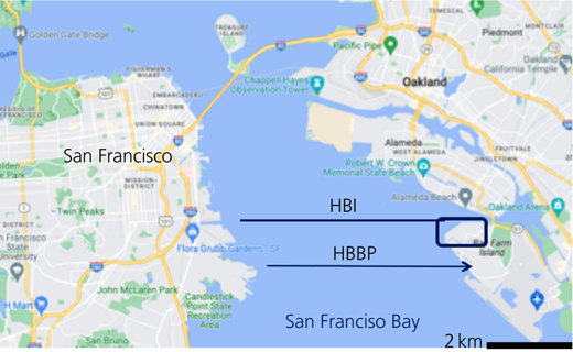
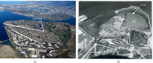
Harbor Bay Isle (HBI) is a residential neighbourhood in the south of Alameda, CA, USA, that was built on land reclaimed from the margin of San Francisco Bay in 1967–1968; the location is shown in Figure 1. The adjacent Bay Farm Island was originally an island in the bay that was settled and farmed in the nineteenth century. The reclaimed area that became HBI lies north and west of Bay Farm Island and comprises about 600 acres (243 ha), with a further 300 or so acres (∼121 ha) reclaimed to the south of the island becoming commercial and office space of the Harbor Bay Business Park (HBBP). Figure 2(a) shows a recent view of the area, looking north towards Alameda from the Oakland airport, while Figure 2(b) is a photograph showing conditions before reclamation started.
Soft estuarine deposits less than 10 000 years old underlie the southern part of San Francisco Bay and the present and former marshlands that border the bay. Known locally as Bay Mud (BM), these sediments infill erosion channels in the underlying sediments that developed during the last glaciation, leading to occasional large variations in BM thickness across the San Francisco Bay region. BM has been investigated in many places for individual developments, with McDonald et al. (1978) collating data from some 2400 boreholes to map the thickness of BM around the bay area. Most of HBI was underlain by BM with as much as 60 feet (ft) (18 m) thickness before reclamation began in early 1967.
The development of HBI provides an unusual case of very soft, high-water-content clay (pre-reclamation void ratios e0 > 2) where land reclamation caused settlements of as much as 2.5 m from about 7 m of sandfill. In the past, the issue for engineers was to predict further settlement when development started, which in this case was some 10 years after reclamation filling, when settlement was continuing at a significant rate. Settlement was also not uniform across HBI, even allowing for the changing BM thickness, with a difference in settlement behaviour between the part of HBI north and west of the sunken ships (which formed part of an early dyke, believed to have been constructed in the 1920s; Figure 2(b)), which was below sea level, and the remainder of HBI where BM was exposed to drying at least some of the time. These areas have been called ‘non-crusted’ and ‘crusted’, respectively (Duncan et al., 1991), with the notion that the crusted area had developed some over-consolidation from desiccation, which was an important contributing factor to the differing settlements between the areas.
This case history became one of two considered in the 27th Terzaghi Lecture discussing deficiencies in consolidation theory and modelling (Duncan, 1993). Identified deficiencies and problems included (a) evaluating pre-consolidation pressures (pc); (b) assessing appropriate consolidation coefficients (cv); and (c) the effect of sand layers and lenses within consolidating strata. The critique of consolidation theory by Duncan (1993) and its application at HBI was based on about 10 years of settlement data from the start of filling. Settlement monitoring has continued since then, and there are now some 43 years of data (see Appendix 1 for a list of records), so what was uncertain at the time development started, and during the time of Duncan (1993), is now known.
This study addresses the issues raised by Duncan (1993) in three ways. First, large-strain theory is used with stress-level dependent properties and explicit representation of time-varying boundary conditions. This is implemented numerically in the Microsoft Excel software program using Visual Basic for Application (VBA) (described later). Second, data from cone penetration tests (CPTs) with an additional pore pressure sensor at the u2 location (CPTu) are used to characterise BM in terms of both over-consolidation ratio (OCR) profiles and division into subunits with individual properties. However, there have been no deep CPTu soundings within BM at HBI and there is no realistic prospect of even research soundings within the modern developed HBI, so soundings are used from other instances of BM, including the nearby HBBP. Finally, because settlement records now extend to the end of primary consolidation, a range of scenarios for properties and in situ pre-consolidation pressures can be evaluated by computing the evolution of settlements and comparing those computed trends with measured data. Iterating across properties allows close fits to measured entire settlement histories, thus the most probable scenario for in situ conditions (including pc) and properties. A feature of this study is using the initial void ratio (e0) to constrain the pre-consolidation pressure profiles, something not addressed by Duncan (1993).
This study focuses on three locations where the BM thicknesses are similar and yet the consolidation histories are markedly different. This choice of just three locations is also a consequence of the destruction of many settlement-monitoring points in the late 1970s with a gap in the record until some settlement markers were restored in 1991. The three locations considered are the only ones with complete records for 43 years that can be used to address the points raised by Duncan (1993).
This case history had original records in ‘English’ units, and some of the figures (particularly elevations) are presented in this form for comparison with these records; the metric equivalent is shown where appropriate. Some of the figures are also scanned from drawings in the day with contours and profiles in feet, which have been used as a base to annotate. Soil properties are given in modern SI units.
Reclamation history and settlement
Smaller-scale reclamation of the Bay Farm area occurred before the 1960s. A portion of what is now HBI was farmed beginning in the late 1920s or early 1930s inside a dyke that began at the western end of Bay Farm Island, ran north and then east and enclosed much of what is now HBI. This dyke was largely formed with ship hulls sunk in place, bow to stern and with added soil (probably excavated BM) between the ships (see Figure 2(b)). The enclosed area was farmed until about 1947, when the dyke was breached and not repaired. Javete (1983) and Duncan et al. (1991) suggested that this period of farming might have created a desiccated ‘crust’. However, the ground surface within the original dyke was low such that the land was inundated by higher tides before the original dyke was constructed and after it was breached (the diurnal tidal range is 6.59 ft (1 ft = 0.305 m) at the nearby National Oceanographic and Atmospheric Administration station 9414750). The land west and north of the original dyke was always submerged beneath San Francisco Bay.
Large-scale reclamation occurred between late 1966 and March 1969, with most of the fill placed within HBI in 1967 and then in HBBP during 1968. The fill was sand dredged from a borrow area in San Francisco Bay, west of HBI, and was largely hydraulically placed within perimeter dykes (the partially completed dyke can be seen in Figure 2(b)) with subsequent use of earth-moving equipment to level the area. The perimeter dykes were constructed as a ‘mud levee’ with a crest elevation of 7.3 ft (2.2 m) above mean sea level (MSL) and with sandfill then placed to an elevation of as much as 9.5 ft (2.9 m) higher than the levee crest at a nominal 10H:1V slope according to the design drawings (the fill was actually thicker in those areas where the top of BM was below MSL). The enclosed area within the dyke had a raised water level to allow fines to settle out in stilling basins. No photographs have been discovered of filling within HBI; ‘beach-above-water’ deposition is apparent for the adjacent HBBP in the photograph shown in Figure 3 with the fill–water boundary at the time highlighted by an arrow and the stilling basin indicated. The photograph in Figure 3 also shows ditches excavated through the HBI to promote drainage of water trapped in the hydraulically placed fill and seeping from the consolidating BM.
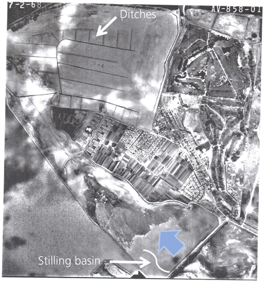
August 1968 view showing drainage ditches in HBI and ongoing filling in HBBP. The blue arrow shows the fill–pond interface within HBBP at the time
August 1968 view showing drainage ditches in HBI and ongoing filling in HBBP. The blue arrow shows the fill–pond interface within HBBP at the time
Fifty-eight settlement plates (SPs; anecdotally 2 ft2 (0.186 m2)) were established on the ground surface throughout the reclamation area before filling, in some instances by dropping the plates through water from a boat. Forty-six plates were in HBI, and the remainder were in the HBBP. Figure 4 shows the history of fill placement from the records at three monitoring points within HBI. The difference in fill thickness between these locations largely reflects differences in the original ground surface elevations as ground generally sloped down from south to north towards the San Leandro channel that borders HBI to the north. Some fill was already in place when the SP elevations were first measured. The subsequent rate of fill placement during the following year suggests that the initial elevation measurements at the SPs ranged from 1 to about 2 months after filling began and with corresponding unmeasured settlements, estimated to range from nominal to about 0.3 ft (0.1 m). The apparent start date for fill placement (t0) at each SP is shown in the figure.
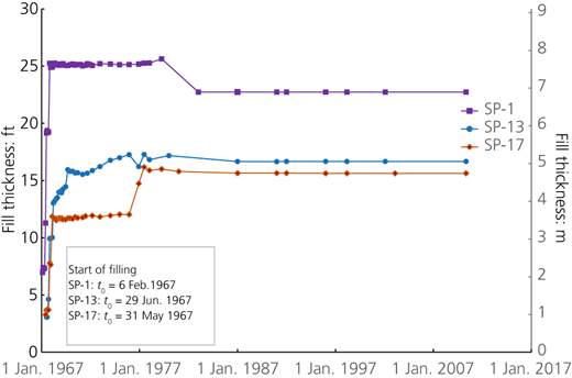
Fill placement at each location was substantially achieved in 1 year but with differing subsequent changes during residential development of HBI throughout the 1980s. In the case of SP-1, regrading after some 15 years reduced the fill thickness by about 2.5 ft (0.8 m). At SP-17, the opposite occurred with an additional 3.5 ft (1.1 m) of fill being placed after 8 years. SP-13 had much of its fill placed in the first year but then accumulated a further 5 ft (1.5 m) of fill over the subsequent 7 years.
Settlements
The SPs were regularly monitored until development started, at which time the plates were destroyed (about 1980 or slightly before). Where possible, measurements were resumed at or near several of the original SP locations using permanent markers placed on project hardscapes that were as close as practical to the original SPs. This resumption of monitoring covered the period 1991–2010; thus, the total record extended to some 43 years after fill placement began. Settlement data were largely contained in reports by surveying companies and found in project files (see Appendix 1). Other settlement data were in the public domain (e.g. Javete, 1983).
Settlement simulations to develop a retrospective view on what would have been the ‘best’ engineering judgement in the day are presented for three locations (SP-1, SP-13 and SP-17), the locations being shown in Figure 5. SP-1 was located in the non-crusted area, while SP-17 was in the crusted area. SP-13 was apparently very near the outside of the dyke created using sunken ships and therefore in the non-crusted area. However, the replaced survey marker may lie east of the dyke and in the crusted area. All three of these SPs were in areas that were flooded at high tide. The BM thickness at each SP is summarised in Table 1 based on adjacent boreholes (data from Javete (1983)). Contours of BM thickness in Figure 5 were developed by the engineers in the day and appear somewhat smoothed with an imperfect match to the borehole records.
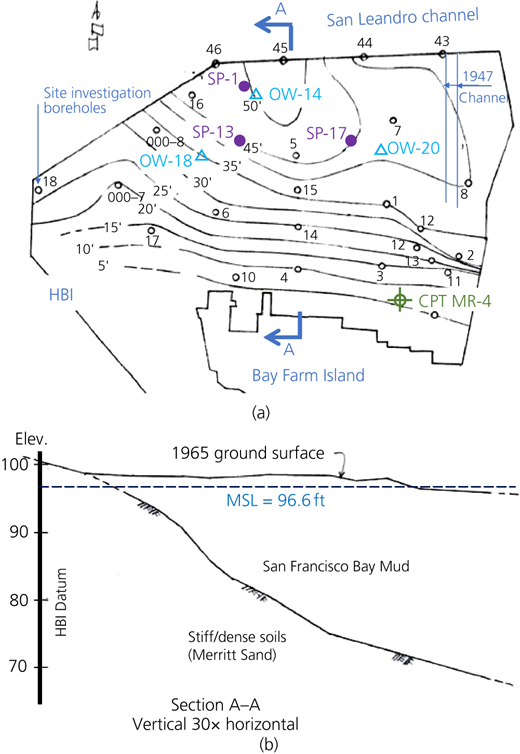
Location of settlement-monitoring points and BM thickness contours (in ft; 1 ft = 0.3 m): (a) site plan; (b) north–south section A–A
Location of settlement-monitoring points and BM thickness contours (in ft; 1 ft = 0.3 m): (a) site plan; (b) north–south section A–A
BM thickness at long-term observation locations (Javete, 1983)
| Location | Start of filling, t 0 | BM | ||
|---|---|---|---|---|
| Thickness | Top elevation: ft | Height above MSL | ||
| SP-1 | 6 February 1967 | 15.2 m (50 ft) | 93.0 | −1.1 m (−3.6 ft) |
| SP-13 | 29 June 1967 | 11.6 m (38 ft) | 99.8 | +1.0 m (+3.2 ft) |
| SP-17 | 31 May 1967 | 13.4 m (44 ft) | 98.4 | +0.6 m (+1.8 ft) |
Note: MSL = 96.6 ft HBI datum; diurnal tidal range 6.59 ft; 1 ft = 0.305 m
The settlement history is shown by the date of observation in Figure 6(a). Primary consolidation was complete after about 30 years, with secondary consolidation then apparent at SP-1 and SP-17 although less at SP-13. Fill was not placed at the SPs simultaneously, so settlement histories did not align by date. The settlement data have been normalised to vertical strain using the thickness of BM at each SP (Table 1) and plotted against log(elapsed time) from the start of fill placement in Figure 6(b) to highlight the transition from primary to secondary consolidation. The final thickness of fill that caused these settlements is indicated (after Figure 4), illustrating the wide range of behaviours between these three SPs.
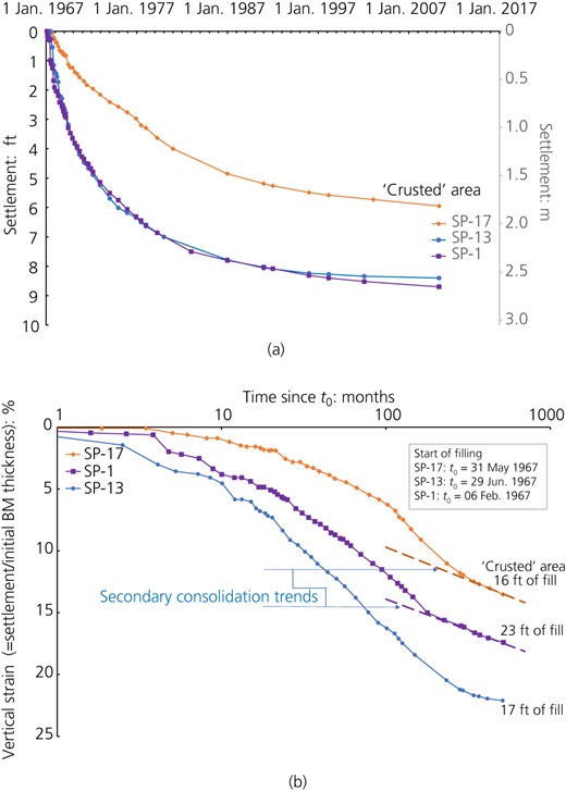
Evolution of settlements with time: (a) settlement plotted against date; (b) settlement plotted against elapsed time from start of filling (log scale) (1 ft = 0.305 m)
Evolution of settlements with time: (a) settlement plotted against date; (b) settlement plotted against elapsed time from start of filling (log scale) (1 ft = 0.305 m)
Stratigraphy and piezometric conditions
Sequence
The HBI area comprised fill, underlain by BM and then generally by Merritt Sand. This sequence was itself underlain by Pleistocene and older sediments to a considerable depth, but these could be neglected to understand the consolidation of BM under the weight of fill used to reclaim the area.
Fill
The fill above the water table was ubiquitously dense, consistent with beach-above-water deposition. The fill unit weights were developed from logs of borings drilled in the south-east corner of HBI as part of a study for a small area within HBI zoned for commercial and office buildings. Data from ten borings gave an average bulk (above the water table) of γ b = 18.1 kN/m3, which became γ sat = 20.5 kN/m3 when saturated.
The groundwater elevations in the fill were measured in observation wells (OWs) near the settlement-monitoring plates, the well locations being shown in Figure 5. These monitoring wells were installed about 14 months after fill placement started, at which time filling was essentially complete, and the wells were then lost when residential development started some 10 years later. At the scale of HBI, OW-14 was close to SP-1 (about 30 m), while OW-20 was a little further from SP-17 (about 100 m). There was no well close to SP-13, with the closest being OW-18 at a distance of about 200 m. Groundwater levels are plotted against dates in Figure 7.
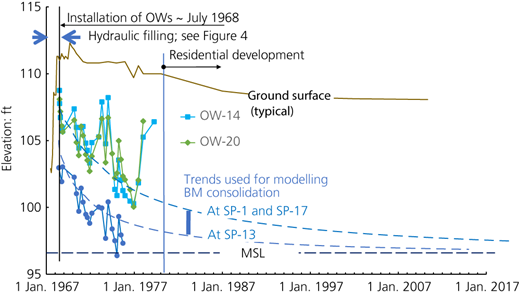
Head within the fill initially increased as a consequence of hydraulic filling followed by a general trend for declining head within the fill between 1968 and 1975. These declining heads were caused by horizontal drainage within the fill, with differing rates reflecting horizontal distances to the drainage ditches apparent in the August 1968 photograph shown in Figure 3. OW-13 appeared to have been close to a ‘spine’ ditch, which would have had a lower elevation than the lateral ditches controlling heads at OW-14 and OW-20.
Data measured in these wells continued beyond 1975 and showed the groundwater rising over the last few measurement years. One explanation of this anomaly was that the winter of 1977–1978 was unusually wet in California, suggesting that infiltration of precipitation into the highly pervious sand might have contributed to a transient increase. As much of the area is now completely developed and covered with hardscape (i.e. houses, streets, sidewalks and the like), it is reasonable to think that the current groundwater elevation within the fill is close to MSL even though the drainage ditches excavated through the fill were backfilled years ago.
Thus, an exponential decay of head within the fill – which was the top boundary condition for vertical seepage – has been adopted for modelling consolidation within BM. These fitted-extrapolated trends are shown in Figure 7 (the trend adopted for SP-13 allows for its location being further from the spine ditch than its paired OW-18).
Bay Mud
Numerous borings in the HBI (see Figure 5) allow for the BM thickness to be contoured, and these contours are shown in Figure 5 along with a north–south section through the HBI. These contours and section are presented in feet, not metres, as that is the dimension used in records of the era (the figure is based on an original record) and consistent with present HBI datum (which has MSL datum = 96.6 ft (29.4 m) at HBI). Broadly, BM thickness parallels the San Leandro channel increasing from about 1.5 m (5 ft) at the southern edge of HBI to more than 15 m (50 ft) where HBI abuts the channel.
There may have been shallow erosion gullies in the surface of the crusted area (Dames & Moore, 1965; Javete, 1983), which were not captured by the contours shown in Figure 5.
A short channel had also been dredged into what is now the HBI during 1947 (Dames & Moore, 1964), also indicated in Figure 5.
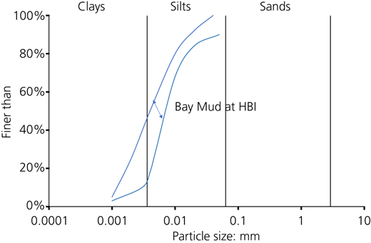
BM is a clayey silt with minimal sand sizes, as shown in Figure 8, but is classified as a high-plasticity clay (CH) in standard index tests with a plasticity index (PI) of 35% < PI < 45% and a liquid limit (LL) of 85% < LL < 88%. The in situ water content is commonly greater than the LL.
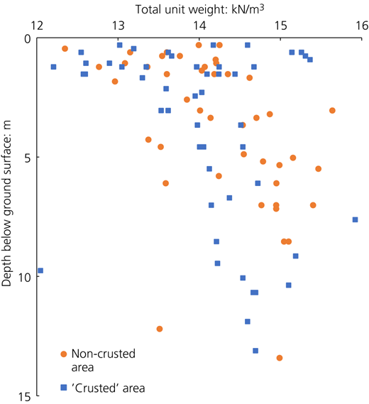
Unit weights for samples recovered in various boreholes put down in HBI are based on the net size and net weight of recovered tube sample (the practice of the time). These weights have been separated into those borings that were in the crusted area and those that were not (Figure 9). No systematic difference in bulk unit weight was apparent between the crusted and non-crusted areas, even in the upper 2 m or so where desiccation would be most expected.
BM is often considered a single geological unit, albeit with stochastic variation of properties such as C c (e.g. Duncan, 1993; Javete, 1983). However, CPTu soundings reveal detail of soil state/property variation and show that what was considered stochastic actually has some systematic arrangement. There were no CPTu soundings during the development of HBI (it predated the modern piezocone, which became available in North America ∼1985), but the CPTu has now become a standard investigation method for BM with numerous soundings across the region. These post-1985 CPTus have been used to assess units within BM.
Figure 10 shows an example of such a CPTu sounding that extends through thick BM overlain by 5 m (16 ft) of fill. This sounding was made at Harrison Street in San Francisco, where the BM is some 25 m thick. Three subunits, A–C, are identified within the upper 15 m at this instance of BM based on the friction ratio F and the normalised induced pore pressure B q, as shown in the figure. Subunits have been identified as showing distinct and common trends in F and B q which ‘jump’ between units, with Figure 11 showing that these identified subunits plot as discrete regions when viewed in a soil behaviour type (SBT) figure (Been and Jefferies, 1992). While some stochastic variation in state/properties is apparent within the identified subunits, each subunit is distinct. There is a sand ‘stringer’ of about 0.5 m thickness at a 20.5 m depth within BM at this location. It is the BM above this stringer that appears most relevant to the 15 m of BM present at HBI.
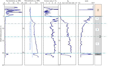
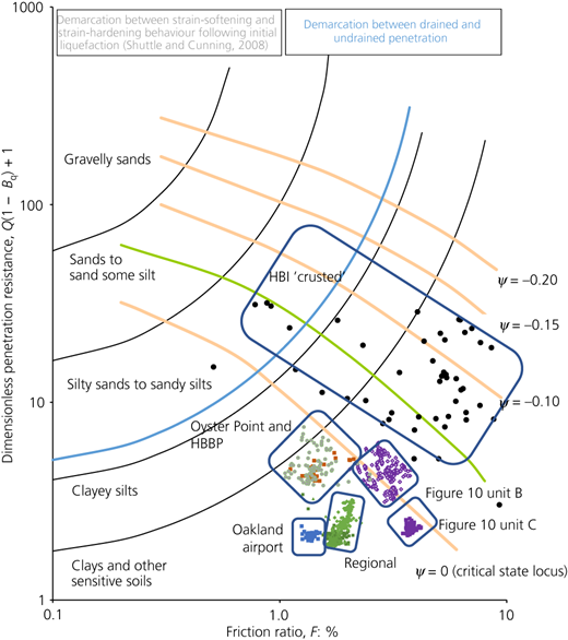
The CPTu profiles in Figure 10 show subunits within BM, and the SBTs exhibited by other instances of BM are helpful in understanding the differences between identified subunits and stochastic variability across a wider occurrence of BM. Figure 11 presents CPTu data from the region extending from Oakland airport through to downtown San Francisco and including the HBBP; different CPTu soundings are distinguished by colour, while different symbols are used for identified subunits within the soundings. Each plotted point corresponds to a single scan, which varies from 20 mm depth increments on some of the soundings to 50 mm increments on others. Several inferences can be drawn from this figure.
The Harrison Street sounding (Figure 10) exhibits three subunits, of which only two are shown for clarity in Figure 11. Harrison Street unit C displays a nearly uniform SBT of a very weak/sensitive silt, while unit B shows both a wider range of SBT and a less compressible soil (C c displays a significant correlation with the friction ratio F (Plewes et al., 1992; Reid, 2015)).
Turning to the Oakland airport sounding, again a very uniform stratum is apparent, much as Harrison Street unit C. Likewise, the deep regional sounding shows two uniform strata (plotted as green squares) but with a third (lighter green diamonds) systematically moving from looser to denser conditions within rather little change in soil type. The Oyster Point and HBBP soundings are very similar. Although some of the variability can be associated with sandier stringers, it appears that the variability in void ratio (see Figure 12) is at least equal in causing the dispersion of SBT seen in Figure 11.
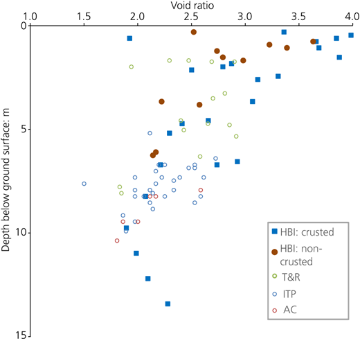
In situ void ratios of BM. Large symbols are within HBI; small open symbols are instances of BM elsewhere
In situ void ratios of BM. Large symbols are within HBI; small open symbols are instances of BM elsewhere
There is one CPTu sounding (MR-4; see Figure 5) within the HBI and that is where the BM is thin (<3.5 m) and in the area reported as crusted from wetting–drying. As can be seen from Figure 11, the behaviour of this shallow/thin crusted BM is very different from that of the deeper BM encountered elsewhere, with the crusted BM showing substantial variability within the profile and with a markedly more dilatant response.
Merritt Sand
The Merritt Formation is a Quaternary dune sand. Gradationally, the Merritt is a fine sand with lenses of sandy clay and clay. It is extensive, underlying Alameda to Oakland, including the HBI, and has been widely investigated for various civil engineering works in the San Francisco Bay area.
The Merritt has been used for wells, and it amounts to an aquifer underlying BM throughout the HBI area. The head in the Merritt was measured in 2003 and was found to be about an elevation of 97 ft (29.6 m), HBI datum, which is slightly above MSL. This has been taken as a constant lower boundary head for consolidation modelling.
In situ state of BM
Void ratios
Water contents were routinely measured during sampling in various site investigations. In particular, there was a considerable body of water content data from borings within HBI. These data have been converted to void ratios using G s = 2.71 (a typical value for BM) and assuming full saturation. The calculated void ratio was plotted against the depth at which the water content was measured (Figure 12). Some of the rather large values in this figure might have been caused by organic content, as the boring logs often contained the statement ‘decayed organics’. Figure 12 also shows void ratio data from three other instances of BM (the locations noted as AC, ITP and T&R), which display exactly the same pattern as that at HBI.
While there is a trend of the void ratio decreasing with increasing depth, as expected, that trend within the upper 10 m is comparable with the large dispersion of void ratios at any depth. Further, there is no apparent desiccation, with crusted and non-crusted samples showing comparable trends and comparable dispersion (indeed, to the eye, it appears the crusted samples are actually slightly looser). The same trends and dispersion are evident at the other various instances of BM tested as shown in Figure 12.
Over-consolidation and pre-consolidation pressure (p c)
The pre-consolidation pressure profile has been assessed using oedometer tests, CPTu soundings and trends in vane-shear strength. These data were discussed in turn before synthesising trends for modelling.
Oedometer
The over-consolidation of BM was determined using oedometer tests on samples recovered from borings at HBI in 1977 using the constant-rate-of-strain (CRS) method (W. N. Houston 1977, personal communication to J. M. Duncan: Report on Consolidation Program on Harbor Bay Isle, Alameda, California). Casagrande’s procedure was used to identify the pre-consolidation pressure, and the results are shown in Figure 13.
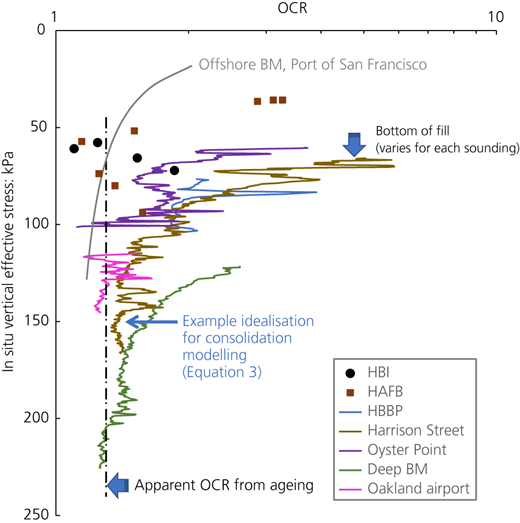
The Hamilton Air Force Base (HAFB) is on the north-western shore of San Francisco Bay, some 20 miles (32.2 km) north of HBI. The BM at this site comprises about 3 m of desiccated sediment underlain by normally consolidated (NC) sediments. Bonaparte and Mitchell (1979) summarised the test data and also noted that the BM properties at HAFB lay between the limits defined at other instances of BM around the bay. Details of the sampling procedures were not known, although it was reasonable to assume that sampling was careful (within the standards of the era), as this was research testing. Both strain- and stress-controlled oedometer tests were used, with Casagrande’s procedure used to identify the pre-consolidation pressure, with the reported pre-consolidation pressures shown in Figure 13.
The pre-consolidation pressures at HAFB and HBI are similar and together suggest a desiccated upper 2 m or so with an average OCR ∼ 3. Below the postulated desiccated zone, a consistent OCR ∼ 1.3 is evident, perhaps a result of ageing (e.g. Bjerrum, 1967).
Inferred from CPTu
The OCR can be assessed directly from the CPTu for cohesive soils based on the notion that the tip resistance reflects the soil undrained strength (the widely used Nkt factor) and that the ratio of undrained strength to confining stress is strongly correlated with the OCR (Ladd and Foott, 1974; Wroth, 1984). However, the tendency in the CPT literature (e.g. Mayne, 2016) is to correlate OCR (generally estimated from oedometer tests) directly with the normalised tip resistance. The approach used here is that suggested by Been et al. (1988), where the tip resistance, normalised by in situ mean effective stress (Qp), is directly correlated with the OCR established from oedometer tests where the pre-consolidation pressure was taken as the yield stress identified from plastic work (Becker et al., 1987), giving
The results of applying Equation 1 to the CPT soundings are also shown in Figure 13 using a ‘not unreasonable’ geostatic stress ratio for soft silts–clays of K0 = 0.7. The sites for the CPTs in Figure 13 include the Oakland airport, Harrison Street and Oyster Point (both downtown San Francisco) and the HBBP adjacent to HBI. The plotted soundings extend from the base of the overlying fill, so that the top of each plotted OCR profile is the fill–BM interface. These CPTs show the same pattern of behaviour, with the OCR decreasing from more than 2 at the top of the BM to become an ‘aged’ value of OCR ∼ 1.3 at depth.
Inferred from vane shear
A feature of prior studies of BM has been a focus on desiccation, both to the degree of induced OCR and the depth to which over-consolidation extends. In this regard, it is interesting to consider an offshore investigation for the Port of San Francisco, where the water depth was about 5 m (18 ft) and the BM appeared never to have been desiccated, as it had always been underwater and was thus in its NC state. The undrained strength (su) of this BM was measured with a vane (Duncan and Buchignani, 1974), and while a clear linear trend of increasing undrained strength with depth was measured, that trend did not go through zero strength at the mudline (figure 2b in the paper by Duncan (2000)). This strength trend implied significant pre-consolidation pressure even at mudline and despite this instance of BM apparently never experiencing desiccation.
The apparent OCR can be computed from a measured strength profile if that profile is compared with the expected profile under truly NC conditions. The idea is embedded in the stress history and normalised soil engineering properties model but is most easily implemented in the form given by Wroth (1984):
where Λ = (Cc − Cr)/Cc. This ratio of plastic to total compressibility tends not to vary with clay type, leading Wroth to suggest Λ ∼ 0.8 as a reasonable approximation for all clays. the oedometer data (Figure 14) give Cr ∼ Cc/7, implying Λ ∼ 0.85 for BM.
The undrained strength ratio of BM has been measured in several studies with the equivalent of unaged (=truly NC) being about (su/p′)NC ∼ 0.33 (an average of the range summarising other studies that was reported by Bonaparte and Mitchell (1979)). Applying this value to the measured linear trend of in situ su using Equation 2 gives the OCR profile shown in Figure 13.
Pre-consolidation pressure trends
The characterisation of ageing inducing OCR in situ through secondary consolidation (creep) by Bjerrum (1967) is well accepted, with Bonaparte and Mitchel (1979) suggesting that an OCR ∼ 1.7 might be expected for geologically aged BM from this mechanism. This OCR would be uniform throughout the profile. However, the CPT soundings discussed above were done after fill placement and commonly two to three or more decades later. Fill placement would disturb the ‘geologically aged’ sediment because the weight of fill would cause stresses exceeding the pre-consolidation pressure, thus restarting secondary consolidation. Bonaparte and Mitchel (1979) measured the creep properties of BM, and these properties suggested OCR ∼ 1.3–1.5 for BM following 30 years of consolidation after fill placement (assuming creep restarts with development of new strains). Because the CPTs in Figure 13 are from post-filling campaigns, the inferred OCR ∼ 1.3 at depth some 30 years or so after fill placement is consistent with filling restarting secondary consolidation.
The developed OCR profiles in Figure 13 – based on oedometer, CPT and vane data – are self-consistent but raise questions about how they developed. The substantial OCR at a shallow depth cannot be attributed to desiccation, as it is present offshore in BM that appears to have been never exposed to desiccation, which is also the case for the non-crusted area in HBI. Further, this apparent OCR from ageing develops immediately below the fill–BM boundary, with the thickness of fill having seemingly little effect.
Most interesting is the OCR trend with depth inferred from vane strengths is similar in form to that derived from the CPTs. The trend annotated as ‘Example idealisation …’ in Figure 13 that captures this form is given by
Equation 3 implies that depositional conditions (wave action?) produced a soil structure that amounts to a constant pre-consolidation pressure over and above that developing from ageing and that depositional-associated pc is not removed by the effective stress increase from filling.
Equally striking, the simple ‘desiccated over NC’ idealisation used by Duncan (1993) for modelling consolidation is far from what the different measurements indicate to be the in situ conditions. Pre-consolidation pressure profiles are treated as an ‘unknown’ to be optimised when modelling the evolution of settlement, with that modelling simulating various idealisations to infer the most likely ground truth.
BM properties
Available data
The two properties of particular interest are the compression index C c and the coefficient of consolidation for vertical drainage c v. Strictly, the hydraulic conductivity (k) is the fundamental soil property, but as both compressibility and conductivity vary together with the void ratio, it is convenient (and conventional) to treat c v (which depends on both C c and k) as a soil property. Both C c and c v are determined from oedometer tests on undisturbed samples, the same tests discussed above in the context of pre-consolidation pressure.
Testing at HBI
Three oedometers tests were carried out on BM well before the reclamation of HBI started (Dames & Moore, 1952), these tests being on either very soft BM or possibly disturbed samples. Only one showed a curve from over-consolidated to NC conditions, with all the samples apparently being on the normal compression locus (NCL) almost immediately and at low effective stress. However, while the rate of consolidation was reported, the sample thickness was not documented, making cv estimates uncertain. A further two samples from the non-crusted area were tested before fill placement (Dames & Moore, 1965).
Sampling and testing after the fill had been placed comprised two standard oedometer tests on samples from the crusted area at the south-east corner of HBI (in the Harbor Bay landing commercial area of HBI (Hallenbeck-McKay and Associates, 1976)) and six strain-controlled (CRS) oedometer tests (W. N. Houston 1977, personal communication to J. M. Duncan: Report on Consolidation Program on Harbor Bay Isle, Alameda, California). These six CRS tests were thought to be as good as could be done in 1977 and provided detailed data on cv and its evolution with the stress level.
Other BM data
Denby (1978) carried out eight oedometer tests, of which two were conventional and six were CRS, on samples from depths of 9–50 ft (2.7–15.2 m) below ground surface at HAFB. However, while detailed compression data were reported, the corresponding data for cv from the six CRS tests have not been recovered. Germaine (2002) carried out three comparable CRS tests on samples of BM and reported such cv data.
Compressibility
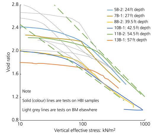
The oedometer data from tests on samples from HBI are presented in Figure 14 in the usual void-ratio-against-log(stress) form. The ‘classic’ semi-log idealisation of normal compression behaviour is evident, with a tendency to reduction in C c (‘reflex curvature’) once . The semi-log idealisation is appropriate for assessing settlements at HBI without any need to consider the evolution of C c at higher stress levels.
Normal compression behaviour can be characterised by 0.8 < C c < 1.1, although C c does not correlate with void ratio (the entire spectrum of C c can be seen at e = 1.6 in Figure 14). The normal compression void ratio (e nc) lies within the limits (shown as dashed lines):
The range of normal compression void ratio is approximately 1.7 < e nc < 2.2 at a vertical effective stress , with no unique NCL for BM being evident in the test data.
Rebound (swelling) behaviour following normal compression was tested in only one sample and then for only a small reduction in stress. Thus, the elastic confined compression behaviour is estimated from the early part of the tests and before the pre-consolidation pressure; a reasonable approximation is that C r ∼ 0.14.
Tests on other instances of BM are shown in Figure 14 as light grey lines. The same pattern of behaviour as at HBI is evident with Table 2 providing compressibility ranges from research studies of BM at HAFB on undisturbed samples.
Summary of oedometer test results on undisturbed samples at HAFB
| C c | C r | Reference |
|---|---|---|
| 0.8–1.2 | 0.12 | Bonaparte and Mitchel (1979) |
| 0.9–1.6 | 0.14 | Bonaparte and Mitchel (1979) |
| 0.8–1.5 | 0.15 | Denby (1978) |
Secondary consolidation
The coefficient of secondary consolidation (C α) was measured for six of the undisturbed sample tests shown in Figure 14, with the load being sustained for about an order of magnitude increase in time. These tests indicated an average C α ∼ 0.01.
Since the interest here is on understanding the effect of various contributing factors to the evolution of primary consolidation, secondary consolidation has been modelled by simply fitting trends to the observed secondary settlements previously shown in Figure 6(b), which gives C α ∼ 0.04 as indicated in the figure. For the range of C c in Equation 4, this calibration to the settlement record gives C α/C c that is essentially the average of experience reported by Mesri and Castro (1987).
Coefficient of consolidation
The coefficient of consolidation, c v, has been determined using both conventional oedometer tests and CRS oedometer tests. In the case of the conventional test, quite different estimates of c v arise from assessing the degree of consolidation at different times, with either t 50 or t 90 being ‘equally standard’. This is a consequence of small-strain theory (the Terzaghi consolidation idealisation) not fitting the rather large strains encountered with consolidation of BM. Equally, the evolution of c v is most conveniently obtained from CRS, but the data reduction used for such tests also relies on small-strain theory (indeed, small-strain theory is embedded in a standard for CRS tests (ASTM, 2020)). Although small-strain theory somewhat compromises the data, such data are all that is presently available and are summarised in Figure 15.
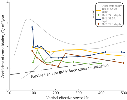
Coefficient of consolidation c v during normal compression of BM (1 ft = 0.305 m)
Coefficient of consolidation c v during normal compression of BM (1 ft = 0.305 m)
Restricting interest to the region stress (which is the in situ conditions within HBI), the CRS data suggest an average c v ≈ 1.3 m2/year with scatter around that value and likely unaffected by vertical effective stress (within the scatter). However, there are no data for . Three tests suggest the possibility of c v increasing as the stress level increases.
The consequence of using small-strain theory to compute c v for soils displaying large compressibility (i.e. where large-strain theory is appropriate) was investigated by Jia et al. (2013), who found that large-strain theory produced consolidation coefficients of about one-half those inferred from the same test data using small-strain theory. This difference in ‘measured’ c v was an effect of large-strain theory capturing the increased hydraulic gradients that developed as the soil compressed (e.g. Gibson et al., 1981). A particularly interesting result was that the soils tested by Jia et al. (2013) exhibited c v that increased with stress when the test data were evaluated using large-strain theory. Their data can be expressed in the form
with an about 50% increase in c v as the vertical effective stress changed from 10 kPa (i.e. top of BM with nominal desiccation) to 300 kPa (=bottom of BM after full consolidation under the fill). A c v trend of this nature for BM as inferred after Equation 5, allowing for large-strain transformation of small-strain data, is shown in Figure 15 using a = 0.7 m2/year and b = 0.0015 (m2/year)/kPa.
Consolidation model
Methodology
The Terzaghi consolidation theory is an instance of the diffusion equation, a standard equation in the applied mechanics literature. In the case of soil consolidation with only vertical drainage, this is
where z is the vertical coordinate; h is the potential (=piezometric head); and c v is the diffusion coefficient (also known as the coefficient of consolidation for vertical drainage). The BM stress–strain behaviour is modelled using a semi-log idealisation for the void ratio, which is expressed in terms of void ratio change de:
A particular feature of consolidation at HBI is the magnitude of strains, which were as much as 23% (Figure 6(b)), requiring more sophisticated mathematics than the usual engineering approximations: large-strain theory. Large-strain consolidation has been developed (Gibson et al., 1981; Jai et al., 2013) in terms of initial coordinates (a Lagrangian system), but such developments have assumed a constant c v, as well as simple boundary conditions. In the case of modelling settlements at HBI, pre-consolidation pressure profiles exist before the behaviour transitions to NC (with a large change in c v) and there is markedly non-linear stress–strain behaviour (Equation 7). Moreover, both loading (=fill thickness) and boundary conditions depend on time. An entirely numerical approach is indicated.
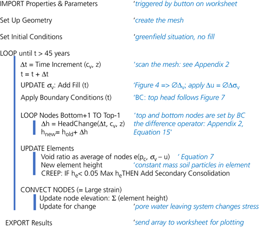
The explicit finite-difference method (Crank, 1956) was adopted with convected coordinates (Gibson et al., 1981); this required a modified difference operator ( Appendix 2). Elements (the soil between the nodes) were associated with a constant mass of soil particles. As pore water flowed from elements, the elements changed both their size and density, reflecting their change in void ratio (full saturation is assumed). The nodes on the element boundaries moved because of the element size changed, and the mesh geometry was updated after each timestep. The solution stepped forward in time in the usual manner for solving the diffusion equation. However, the timestep must be varied from step to step for numerical stability because of changing geometry and changing c v (c v is taken as constant during a timestep).
The finite-difference solution was programmed in VBA, a high-level language that was provided with the Microsoft Excel software program (accessed through the ‘Developer’ option); the flow chart for the code is given in Figure 16. Input was controlled from the Microsoft Excel program, the solution computed entirely within VBA, and the results were transferred to a worksheet for plotting and comparison with the measured settlement history being simulated. Each simulation computed in a few seconds.
Idealisation for HBI
The consolidated stratum was represented by 100 soil elements (=101 nodes), initially at equal heights and with a fixed bottom boundary (conceptually the top of the Merritt Formation).
The bottom boundary was taken as the prescribed head, consistent with Merritt Formation acting as an underdrain to BM. The top boundary was free draining but with a declining head over time. The trends shown in Figure 7 were used with a linear increase in head during hydraulic filling as the fill increased in height.
The initial void ratios are taken as the following semi-log laws:
where e pc is the void ratio on the NCL at while e 1kPa is the void ratio on the NCL at . Thus, e 1kPa sets the ‘altitude’ of the modelled NCL within the spectrum of oedometer data (see Figure 14) and is a property used in iterating so that every idealisation falls within the spectrum of the measured behaviour (see Tables 3 and 4).
Summary of scenarios for SP-13 with BM as single stratum
| Model property | Scenario A: aged OCR | Scenario B: Figure 13 OCR with offset | Scenario C: c v increasing with |
|---|---|---|---|
| Top (HBI datum) | 99.82 ft (30.44 m) | 99.82 ft (30.44 m) | 99.82 ft (30.44 m) |
| Thickness: m | 11.58 | 11.58 | 11.58 |
| Crust | None | None | None |
| NCL | |||
| OCR or p c | OCR = 1.18 | OCR = 1.15 | |
| c v | 1.3 m2/year | 1.7 m2/year | |
| Creep | Cα = 0.04 | Cα = 0.04 | Cα = 0.04 |
Note: top elevations and stratum thicknesses are initial values
Summary of best-fit idealisations with BM as two subunits
| Model property | SP-1 (Scenario G) | SP-13 (Scenario D) | SP-17 (Scenario E) |
|---|---|---|---|
| Top subunit of BM | |||
| Top | 93.03 ft (28.37 m) | 99.82 ft (30.45 m) | 98.43 ft (30.02 m) |
| Thickness: m | 4.50 | 6.5 | 6.0 |
| Crust | None | None | None |
| NCL | |||
| OCR or p c | 1.05 | ||
| c v: m2/year | 0.95 | 0.90 | 1.00 |
| Creep | Cα = 0.05 | Cα = 0.05 | Cα = 0.05 |
| Bottom subunit of BM | |||
| Top | 78.23 ft (23.86 m) | 78.42 ft (23.92 m) | 78.75 ft (24.02 m) |
| Thickness: m | 10.74 | 5.08 | 7.41 |
| NCL | |||
| OCR or p c | 1.05 | ||
| c v: m2/year | 1.70 | 1.80 | 1.80 |
| Creep | Cα = 0.05 | Cα = 0.04 | Cα = 0.04 |
Note: top elevations (HBI datum) and stratum thicknesses are initial values
The fill height at any time follows a piecewise linear fit to the record (Figure 4), including reductions in fill height that occurred after some 10 years at SP-1 and the increase at SP-17.
Secondary consolidation was started once the excess head had reduced to 5% of its maximum excess at the middle of any element. Thus, elements did not enter the secondary stage at the same time.
Iteration
Analysis of these long-duration settlement records used iterative forward modelling where properties/parameters were estimated, settlement was computed for these estimates and then the properties/parameters were updated (‘iterated’) to fit the measured data better. Iteration was constrained by the oedometer data and in situ water contents to identify the most probable ground truth.
Parameters varied
Assessment of HBI settlement in the literature (e.g. Duncan et al., 1991) has looked at the effect of desiccation as a key differentiator between the various SPs during BM consolidation: the crusted against non-crusted hypothesis. However, there were other possibilities. Ageing appeared neglected with the possibility of an apparent OCR > 1 throughout BM, as shown in Figure 13. Within any desiccated BM, there was conflicting evidence as to how pre-consolidation pressure changed with depth (Figure 13).
The duration of monitoring was sufficiently long that primary consolidation finished. As settlement is a strong function of C c, this means that an average C c is defined in any simulation so as to match the observed end-of-primary settlement. However, there is an uncertainty as to whether there are two or more-subunits within BM (e.g. as per Figure 10), in which case different values of C c can be invoked subject to their combination giving the required settlement match to data at 30 years or so. To keep scenarios manageable, only two layers were adopted as a scenario for simulation. Consistent with the void ratio data at the site, the lower of the two layers was taken as the denser and stiffer one.
The third aspect considered was the coefficient of consolidation c v, with values adjusted to match the observed settlement rate in any scenario.
The choice of the three SPs also defines the scenarios. SP-1 is clearly non-crusted from its proximity to the San Leandro channel and the surface of the BM being below MSL. However, a consequence was that an unusually large amount of fill was placed at SP-1. Thus, analysis started with SP-13, which was thought to be an uncrusted location and which displayed the largest vertical strains of the SP (see Figure 6). SP-17 represented the crusted scenario advocated as key to understanding HBI settlements by Duncan (1993). These chosen SPs indicated that SP-13 should be considered first as the ‘greenfield’ case and then SP-17 to investigate crusted effects while attempting to honour the situation at depth found in SP-13. Finally, SP-1 raised the issue of the largest amount of fill not causing the largest vertical stain (see Figure 6).
Numerous simulations were carried out within these broad aspects (each simulation ran in a few seconds). The properties and geometry iterated were whether there were subunits within the BM or not and, if so, the depth of the boundary between them; the initial void ratio profile; the pre-consolidation pressure profile; C c and C r for each subunit; and c v for each subunit including stress-level dependence. Distinct scenarios were reported here to highlight how the best fits were developed. The individual fill height against time and groundwater level in the fill were honoured in detail in all simulations. These differed among the three SPs, as shown in Figures 4 and 7.
Results
The simulation results for each scenario are presented on a single figure comprising three plots: the computed settlement–time history as ‘plot (a)’; the computed void ratio profile as thick coloured lines superimposed on the data of Figure 12 (with data now in light grey) as ‘plot (b)’; and the evolution of void ratio with vertical effective stress as thick coloured lines for two nodes, the upper one set at 25% depth (node A) and the second one at 85% depth (node B), compared with oedometer data of Figure 14 (now light grey), as ‘plot (c)’. The initial depths of the nodes are shown on the ‘(b)’ plots.
Non-crusted: SP-13
Four scenarios were defined at SP-13. Scenario A was for a single stratum of BM with uniform C c and c v with a simple aged pre-consolidation pressure profile. Scenario B was similar but changed the pre-consolidation pressure profile to simulate that inferred from CPT and vane-shear data discussed previously; see ‘Example idealisation…’ in Figure 13. Scenario C looked to c v depending on the stress level as inferred possible from the evaluation of oedometer data using the inferred trend shown in Figure 15. Figure 17(a) shows the computed evolution of settlement with time and compared with that measured at SP-13 for the three scenarios A–C. Figure 17(b) shows the distribution of void ratio with depth corresponding to the soil properties and pre-consolidation pressure. Figure 17(c) gives the results for the evolution of void ratio at the two nodes monitored. The best-fit properties for these three scenarios are given in Table 3.
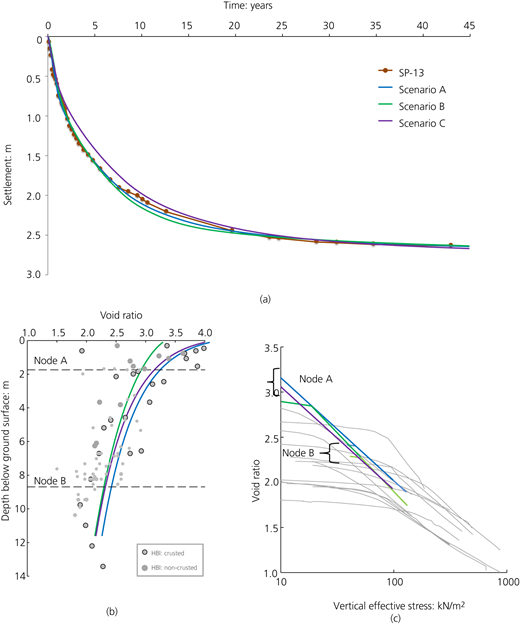
Computed behaviour for SP-13 in scenarios A–C: (a) computed settlement–time history; (b) modelled void ratio profile; (c) evolution of void ratio with vertical effective stress
Computed behaviour for SP-13 in scenarios A–C: (a) computed settlement–time history; (b) modelled void ratio profile; (c) evolution of void ratio with vertical effective stress
Scenario A provided a reasonable fit to the measured settlement using an ageing OCR = 1.18 (which is plausible for geological ageing) and compression behaviour that was near the average of that measured in the oedometer tests. However, while measured void ratios are honoured in the upper 5 m or so of BM, the simulated consolidation was far too loose at depth. Further, while the evolution of settlement was captured within the first 6 years, the computed trend in the period of 7–15 years was less impressive.
Scenario B was a poorer fit to the measured settlement than A, albeit with an arguably better match with in situ void ratios.
Scenario C was also a poorer fit than A for the initial 8 years or so, although the trends for increasing settlement with time were interestingly similar in the 10–20-year period.
The results shown in Figure 17 led to scenario D, which adopted two subunits within BM. The boundary between the two subunits was set at a 6.5 m depth based on the in situ void ratio trends. The two subunits were given different properties, idealising the lower unit as denser and stiffer (the lower node) than the overlying very soft BM (the upper node). The computed settlement trend is given in Figure 18(a). The computed behaviour laid virtually on top of that measured with close honouring of changes in the rate of settlement. The primary consolidation settlement was also indicated, illustrating the contribution of secondary consolidation during the period when the area was developed. Figures 18(b) and 18(c) show that the computed void ratios are now plausible representations of the in situ and oedometer data. This is the best fit achieved, and these properties/parameters are given in Table 4. Interestingly, introducing a denser lower subunit has the effect of requiring a lower OCR to match the measured settlements (compare Table 3 with ‘D’ in Table 4).
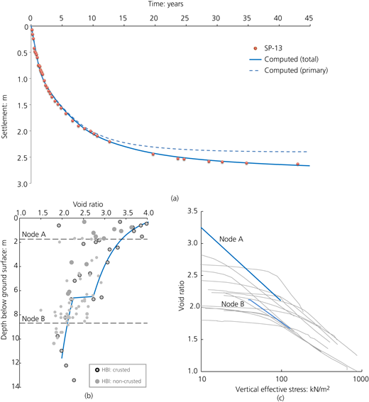
Results of scenario D (=best fit) for SP-13: (a) computed settlement–time history; (b) computed void ratio profile; (c) evolution of void ratio with vertical effective stress
Results of scenario D (=best fit) for SP-13: (a) computed settlement–time history; (b) computed void ratio profile; (c) evolution of void ratio with vertical effective stress
Crusted: SP-17
The starting point for modelling SP-17 was the property set of the best fit for SP-13 (Table 4), maintaining the same elevation for the upper/lower subunit boundary and with over-consolidation introduced. Thus, the notion that some of the different behaviours between the three SPs considered were a consequence of the differing thickness of the upper soft subunit.
There are two contrasting ideas about over-consolidation in the crusted area: honouring the denser trends of the measured in situ void ratios (scenario E) or desiccation of the upper 2.5 m with consequent induced pre-consolidation from capillary tension (scenario F). In scenario E, there is no ‘crust’ as such, rather a shift to a denser void ratio trend throughout the BM. In scenario F, dense BM (the ‘crust’) is a distinct layer that overlies wet (but possibly aged) BM. The results of the iterated fits for these two scenarios are shown in Figure 19.
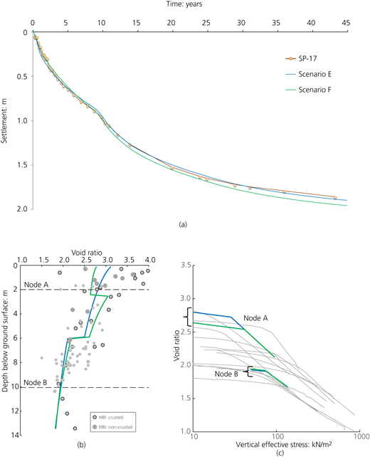
Computed behaviour for SP-17 in scenarios E and F: (a) computed settlement–time history; (b) computed void ratio profile; (c) evolution of void ratio with vertical effective stress
Computed behaviour for SP-17 in scenarios E and F: (a) computed settlement–time history; (b) computed void ratio profile; (c) evolution of void ratio with vertical effective stress
Scenario E easily fitted the measured settlement trend (Figure 19(a)), using a slight modification of Equation 3 to smaller coefficients (see Table 4), which produced a reasonable fit to the denser void ratios throughout the upper subunit, as shown in Figure 19(b). In this scenario, the compression behaviour with stress was similar to the best fit at SP-13 (in both subunits) but with a greater proportion in the C r regime because of more over-consolidation. The c v values were also similar to those at SP-13.
For scenario F, a 2.5 m thick crust was used with the void ratio chosen to the denser end of the measured in situ data (see Figure 19(b)). This void ratio choice then produced the p c profile from mapping the void ratio to the chosen NCL (which was the same as calibrated for the upper subunit at SP-13). Initially, the OCR profile below the crust was set as nominally NC, but while the crust minimised strains within it compared with the uncrusted situation, settlements were much larger than reality because the BM below the crust remained soft with C c ∼ 1. Iteration then proceeded by increasing OCR in the BM below the crust to match that computed with measured settlements. The simulation shown in Figure 19 as scenario F used OCR = 1.5 below the crust, which was substantial geological ageing as discussed previously but not implausible. However, while a good fit was evident for the first 10 years, at later times, progressively greater settlement than measured were predicted. No parameter combinations were discovered that kept the good early-time fit while improving on late-time behaviour. Thus, the judgement that scenario E was the best fit for SP-17 and the properties used are given in Table 4.
High fill: SP-1
SP-1 was located near the San Leandro channel and with the top of the BM about 2 ft (0.6 m) below MSL – an area that was flooded daily. Two scenarios were considered for ageing: scenario G, comprising the pre-consolidation pressure profile implied by CPT data (i.e. Equation 3), and scenario H with a uniform OCR. The soil properties for both G and H started with those that were the best fit at SP-13 and with only minor adjustments subsequently. The notion that the top of the lower subunit of BM was level across the site was adopted. The computed settlements are shown in Figure 20(a).
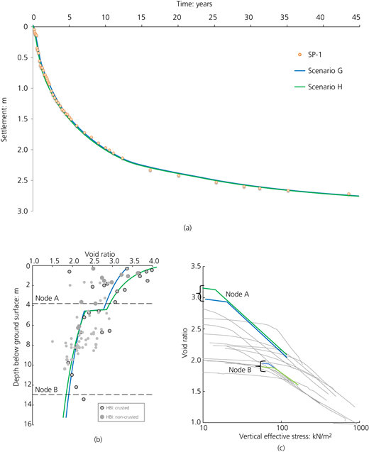
Computed behaviour for SP-1 in scenarios G and H: (a) computed settlement–time history; (b) computed void ratio profile; (c) evolution of void ratio with vertical effective stress
Computed behaviour for SP-1 in scenarios G and H: (a) computed settlement–time history; (b) computed void ratio profile; (c) evolution of void ratio with vertical effective stress
The OCR idealisation for scenario G started with Equation 3 but then required reducing the coefficients to fit the measured trend. Scenario H simply iterated on OCR with a uniform ‘aged’ OCR = 1.45 giving the fit shown in Figure 20(a). At first glance, it was difficult to distinguish between the two scenarios in terms of fit to measured values, but a close inspection showed that G gave a better fit in the first 4 years before the two scenarios then becoming practically indistinguishable. However, the scenarios differed in their fits to void ratio data, with scenario H focused to the very loosest values that might be a consequence of organic content (as noted earlier). On balance, scenario G seemed preferable, and the values used in the scenario are given in Table 4.
Discussion
While large-strain theory improves predictions of soil consolidation, arguably the most important aspect was not large-strain theory per se but rather its numerical implementation with detailed capture of time-varying boundary conditions. The fill placement history (Figure 4) showed that regrading of the HBI just prior to development added 4 ft (1.2 m) of fill at SP-17 and removed 3 ft (0.9 m) of fill at SP-1. At SP-17, this modest additional fill produced a marked increase in the rate of settlement that was fully captured by the numerical simulation (Figure 19(a) at ∼10 years). At SP-1, removal of this small amount of fill ended primary consolidation with a sudden decrease in the settlement rate that was also fully captured by the numerical simulation (Figure 20(a) at ∼14 years). Accurate assessment of the potential for future differential settlement requires accurate modelling (and records) of filling and regrading history.
Table 4 collates the best-fit properties developed for the three SPs. Reiterating, the idealisation of BM into two subunits is supported by the systematic difference in SBT seen with the CPT at various instances of BM elsewhere and in particular within individual soundings (see Figures 10 and 11). The oedometer data show a wide band of NC behaviour (Figure 14), and the scenarios explored have assigned the denser oedometer trends to the lower subunit, consistent with the in situ void ratios, while the looser oedometer trends have been associated with the upper subunit. Thus, the measured spectrum of oedometer compression behaviour is included in the simulations.
The notion that the top of the lower subunit might present a consistent elevation across the HBI (Table 4) implies the differences in settlements between the three SPs are partly caused by the differing thickness of the more and the less compressible BM at each SP. It is interesting that rather similar NCL behaviours are developed for the two subunits at all three modelled SPs (Table 4) with this notion. Returning to the critique of consolidation theory by Duncan (1993), if accurate settlement predictions are required, then start with a campaign of CPTu soundings to define the geological detail of the consolidating strata (of course these CPTus were not available before 1985, but two subunits within BM could have been developed from the available water content data).
The prior analysis of the HBI settlements by Duncan (1993) and Duncan et al. (1991) suggested that the presence or absence of a desiccated crust was central to understanding the differences in settlements at the various SPs. Detailed modelling does not support this hypothesis – the crust on its own is insufficient to reduce overall settlement. Furthermore, the ‘crust over normal consolidated’ idealisation simply does not match the numerous void ratio data.
Although subunits within BM (for which there is abundant evidence in addition to the excellent fits achieved) appear central to the differing settlements at HBI, there is clear presence of apparent pre-consolidation from ageing over ‘geologic’ time before filling started. While ageing is commonly considered in the form suggested by Bjerrum (1973), which amounts to an apparent uniform ageing-induced OCR with depth, such an effect of ageing in inconsistent with in situ tests on BM elsewhere. Moreover, choosing an effect of ageing that fits the trends shown in those in situ tests (Equation 3) produces plausible matches to in situ void ratios measured at SP-1 and SP-17 (Figures 20(b) and 19(b), respectively). SP-13 is different, exhibiting little ageing while matching the loosest instances of BM at HBI (Figure 18(b)). Figure 21 compares these inferred pre-consolidation pressure profiles. These profiles are consistent with what is apparent when CPT data are processed to infer over-consolidation profiles (Figure 13 and Equation 3). In particular, Figure 13 implies depositional effects, which are not removed by subsequent loading. Of course, a limitation of this study has been the absence of CPTu data close to any of the SPs considered. Further CPTu soundings are needed within the HBI (if access could be gained) to understand this case history fully.
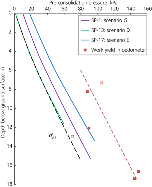
Inferred in situ pre-consolidation pressure profiles from best fits achieved
Inferred in situ pre-consolidation pressure profiles from best fits achieved
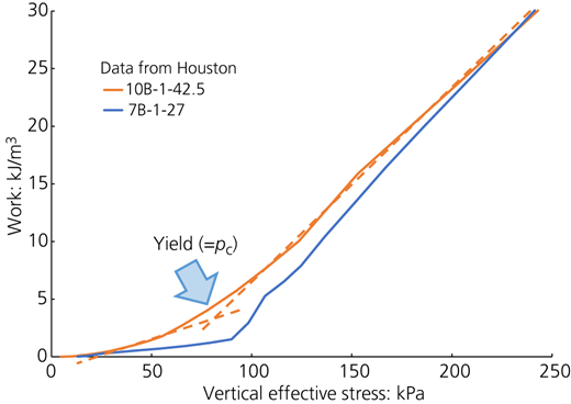
The pre-consolidation pressure affects settlement as it proportions the loading between elastic (Cr = small strains) and elastoplastic (Cc = larger strains) regimes. The oedometer tests within the BM at HBI were reviewed, using the notion of work to identify the pre-consolidation (= yield) pressure – the methodology introduced by Becker et al. (1987). Figure 22 shows example results. The test shown in blue has a clear change in the rate of working as stress increases, associated with the change from the stiff elastic regime to the softer elastoplastic regime; this is the yield condition of plasticity. However, the test shown in brown produced a gradual transition with yield taken from the intersection of the linear trends in elastic and elastoplastic regimes (shown as dashed lines in the figure).
The yield stress determined for the six HBI oedometer tests is plotted against sample depths in Figure 21, with open symbols for the samples showing gradual onset of plasticity and solid symbols for instances of reasonably sharp yield.
It is apparent from Figure 22 that this retrospective processing of the oedometer data still results in only two of the six samples matching what is needed from observed settlements. An aspect of BM is that, while it is classified as a high-plasticity clay, it presents in CPT soundings as a sensitive silt. Sensitive silts can densify during sample extrusion and handling, with the resulting void ratio reduction then presenting as an increase in yield stress: a sand-like behaviour. If the oedometer yield is taken at face value, computed settlements are only about three-quarters of those measured even using a biased high Cc ∼ 1.1 throughout BM and with in situ void ratios then no longer honoured.
To some extent, the ‘issue’ of pre-consolidation pressure arises as a consequence of idealising soil compressibility as two semi-log regimes: elastic (controlled by Cr and pc) and elastoplastic (controlled by Cc). The pre-consolidation pressure is simply the intersection of these regimes. There is a case for using a soil model that more closely follows the gradual transition from elastic to fully plastic behaviour (i.e. representing the curved oedometer trends), but such an approach is far from current practice. More research (and theory) would be helpful. For now, it appears better to estimate a pc profile from analysis of case histories – such as this one – for the geological situation of interest than using oedometer data. Of course, that depends on the availability of such data, but in turn, that implies an engineer should have a continuing interest in the performance of works in their region of practice.
The cv values were iterated to match the measured rate of development of settlements. This provided further support for the two subunit hypothesis as, while a single stratum could fit measured trends at SP-13, better fits at SP-13 and excellent fits elsewhere were achieved using two subunits, each of which had a different cv (compare scenario A in Figure 17 with Figures 18–20). In effect, the subunit idealisation allows two parallel time factors for dissipation of excess head. These cv values differ from the oedometer results, as shown in Figure 23, which was expected because oedometer data are reduced using small-strain theory (embedded in the American Society for Testing and Materials standards for oedometer testing), which neglects the larger gradients of reality, which are included in the large-strain approach used in this study.
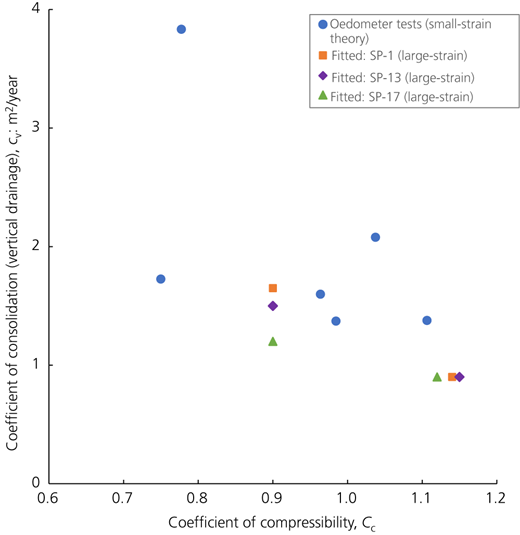
Comparison of consolidation properties from CRS oedometer tests with those inferred from best-fit simulation of measured settlement histories (large strain)
Comparison of consolidation properties from CRS oedometer tests with those inferred from best-fit simulation of measured settlement histories (large strain)
Finally, Figure 18(a) shows that much of the late-time settlement is secondary (creep). Returning to the question, ‘What would have been the best judgement in the day?’, this study has simply fitted secondary consolidation trends and not predicted them. Using an average Cα/Cc ratio from experience (i.e. Mesri and Castro, 1987) would have predicted behaviour close to that observed, but there is scatter in that experience and nothing specific to indicate why an average might have been expected to be a ‘good choice’. Thus, Duncan’s critique of consolidation theory should be extended as present understanding of secondary consolidation warrants further research leading to proper mechanics for the process.
Supplementary data
The VBA code appears within Microsoft Office as a ‘macro-enabled’ file, a form that this journal precludes as supplementary data because of the potential for transmitting viruses. Contact the authors for further information to produce Figures 18–20.
Conclusion
The nearly 45-year history of settlement monitoring at HBI is unusual in that (a) it fully captures primary consolidation with transition to secondary creep and (b) BM exhibits high void ratios and some of the largest compressibility of soils in the literature. Iterative forward modelling based on large-strain theory was used to infer in situ properties and state, with the modelling constrained by measured in situ void ratios and the spectrum of behaviour in oedometer tests on undisturbed samples.
The idealisations adopted relied on in situ tests at other instances of BM. The reclamation that became HBI was some 15 years before the CPTu became available, and the thickly settled development of HBI effectively precludes subsequent ‘research’ testing. However, BM has proved consistent regionally and the CPTu data are clear that BM is not a single geological unit. This is also consistent with water content data from the original site investigations.
The iterative modelling, treating BM as two distinct subunits, achieved plausible fits to measured in situ void ratios at HBI while giving close matches to the settlement histories over 43 years. No support was found for the hypothesis that the presence or absence of desiccation was a key differentiator for the evolution of settlements. Rather, it is the proportion of loose and denser subunits that is important with a further effect of ‘ageing’. The iterated pre-consolidation profiles suggest that, while ageing in the sense of Bjerrum (1967) is a factor, depositional conditions during accretion of the BM have resulted in a residual fabric that presents as an additional component to the pre-consolidation pressure.
Appendix 1 Sources of settlement data (from authors’ files)
Dames & Moore, 16 February 1965, report for Bay Farm Reclamation District 2105, soil investigation, proposed Bay Farm Island development, Alameda, CA
Dames & Moore, 27 March 1964, letter to Utah Construction and Mining Company, consultation, compilation of available data, Bay Farm Island, Alameda, CA
Dames & Moore, 14 January 1952, report for the Utah Construction Company, soil investigation and reclamation studies, Bay Farm Island project, Alameda, CA
Duncan JM, 1 July 1977, letter to Mr Oscar Barry, summary report on differential settlements at tract 3645, HBI – Village II
Duncan JM and Houston WN, 8 July 1977, report for Harbor Bay Isle Associates, differential settlements at tract 3645, HBI, Village II
Hallenbeck-McKay and Associates, 15 October 1976, report for Bedford/Lafayette Investment Services, soil and foundation investigation, HBI market place, community centre park–HBI, Alameda, CA
Hallenbeck and Associates, 6 February 1986, letter to Bedford Properties, geotechnical engineering study, Harbor Bay Shopping Center – phase 2, Harbor Bay Landing – Alameda, CA
Hallenbeck and Associates, 4 May 1992, report for M. A. Lindquist Company, geotechnical engineering investigation and design recommendations, HBI community centre, Alameda, CA
Jensen-Van Lienden Associates, 21 May 1991, report for Design Planning Associates, geotechnical engineering investigation, proposed community of HBI office building, Alameda, CA
Jensen-Van Lienden Associates, 3 April 2003, report for Bay Farm Community Church, geotechnical engineering study, proposed new addition, Bay Farm Community Church, Alameda, CA
Jensen-Van Lienden Associates, 11 December 2008, report to Clear Channel Outdoor, geotechnical engineering study, foundation conditions, 971 Harrison Street, San Francisco, CA
Jones-Tillson & Associates, 24 February 1969, amended reclamation plan, Reclamation District 2105, Bay Farm Island, Alameda, CA
Jones-Tillson & Associates, December March 20, 1967, SP locations, reclamation district 2105, Bay Farm Island, Alameda, CA
Jones-Tillson & Associates, December July, 1977, SP locations, reclamation district 2105, Bay Farm Island, Alameda, CA
Jones-Tillson & Associates, December January, 1982, SP locations, Reclamation District 2105, Bay Farm Island, Alameda, CA
Jones-Tillson & Associates, undated, SP locations, Bay Farm Island, Reclamation District 2105, subsidence graphs
Michelucci & Associates, 16 March 2023, report to Clear Channel Outdoor, geotechnical engineering study, proposed digital advertising sign, 1 Oyster Point Boulevard, South San Francisco, CA
Robert A. Day Land Surveying, 7 March 2002, community of HBI, settlement point readings
Robert A. Day Land Surveying, 17 June 2010, community of HBI, settlement point readings
Appendix 2 Finite-difference operator for diffusion on a non-uniform mesh
The Terzaghi consolidation theory is an instance of the diffusion equation, a standard equation in the applied mechanics literature. In the case of soil consolidation with only vertical drainage, this is
where z is the vertical coordinate; h is the potential (=piezometric head); and c v is the diffusion coefficient (coefficient of consolidation for vertical drainage).
A finite-difference mesh of N nodes is used; elements of constant mass of soil particles lie between the nodes (thus, N − 1 elements). Node j is at location z j and has head h j. First-order (linear) discretisation is adopted.
Considering discretisation in space, at the element above node j, the head gradient at the centre (location ‘+1/2’) of this element is
and similarly for the element below node j.
At node j, the spatial rate of change of head gradient is
As z j +1/2 = (z j +1 + z j)/2, then Equation 11 can be written as
Equations 10 and 12 show that head and height information is needed at the nodes.
Turning to discretisation in time, at node j
Using Equations 11 and 13, Equation 9 becomes approximated as
which expands into
All the terms on the right-hand side of Equation 15 are known at time t at nodes j: 2 to (N − 1). The head at nodes 1, N comprises the boundary conditions, also known. The solution is progressed by stepping forward in time using steps of Δt.
The approximation of the continuous h(z,t) with finite differences amounts to using the first term of the Taylor series expansion (Crank, 1956), with then a need for the effect of the omitted higher-order terms dying out with time to avoid numerical instability. This leads to the requirement that
The requirement of stability varies at every node because of changing geometry (the convected coordinate approach to large strain) and c v varying with stress, in particular by about an order of magnitude change between elastic and elastoplastic nodes. Thus, the mesh must be scanned at every timestep with the smallest Δt then governing

