


The pressuremeter holding test may be used to determine the consolidation characteristics of clays and, once certain other parameters are known, the permeability. These other parameters, the shear strength and modulus, may be ascertained from the expansion part of the test. Various methods of analysis have been proposed in the past, and they are compared here. The similarities to the piezocone dissipation test are explained, and the analysis methods are compared. A new method of analysis is described, using an Excel spreadsheet that simulates the pressures and flows around a cylindrical object.
Notation
- A, B, M
constants
- CH
coefficient of consolidation
- Cu
shear strength
- CV
coefficient of consolidation
- Eν
bulk modulus (connected to the shear modulus G by Poisson’s ratio)
- G
shear modulus
- IR
rigidity index (G/C u)
- k
coefficient of permeability
- m
normalised slope (S o/U o)
- mv
volume compressibility (1/E v)
- Pmax
pressure at start of hold
- r
radius of measurement
- ro
radius of the expanded probe
- R
radius of failed zone
- S
slope of the plot of pore pressure against ln t
- Smax
maximum slope of the plot of pore pressure against ln t
- So
slope of the plot of pore pressure against √t
- t
elapsed time
- t50
measured time to 50% consolidation
- T50
time factor for 50% consolidation
- T90
time factor for 90% consolidation
- Uo
maximum pore pressure generated
- Ur
excess pore pressure at radius r
- V
current (i.e. expanded) volume of the probe
- γw
unit weight of water
- ΔV
increase in volume
- ν
Poisson’s ratio
Introduction
The pressuremeter is a versatile tool for in situ testing, which may be used to determine many basic soil properties. Interrupting the standard test procedure, to hold either the pressure or expansion constant, allows further information to be discovered on creep or consolidation (and hence permeability).
Holding the expansion constant gives a situation which is analogous to a piezocone dissipation test and which may be analysed in exactly the same manner. Various methods of analysis are compared, and potential problems are highlighted.
The original work on these analyses involved some fairly powerful mathematics; in this paper, the author shows how the dissipation can be modelled using a standard Excel spreadsheet and simple physics. This allows various relationships to be determined, both confirming the original work and leading to a new method of analysis where a computer-generated curve is matched to the test data.
Of the two types of pressuremeter holding test, the pressure hold is the more obvious – the applied pressure is held constant and the continued expansion is monitored. This gives information on the creep and can be used in rocks as well as soils. It can be shown that the creep settles rapidly and may be used to predict long-term behaviour.
The strain hold is what is of concern here, as it may be used to determine consolidation and hence the permeability of clays. It has been much studied, over many years, and the theory behind it is well documented. There are many papers on the subject, principally by members of the Soils Group at Cambridge University.
To perform this holding test, the pressuremeter is expanded until sufficient pore pressure is generated; then, the expansion is held constant and the decay of excess pore pressure is monitored. There are thus two key requirements for a successful holding test – the ability to maintain a constant expansion and the ability to measure the pore water pressure generated by that expansion.
The self-boring pressuremeter (SBPM), designed and manufactured by Cambridge Insitu Limited, has the necessary features to accomplish this task – it has pore pressure cells embedded in the pressuremeter membrane and an output of the ‘total strain’ which can be used to feed the strain control unit. This piece of equipment was designed to give constant rates of expansion or contraction – one of which is zero. It adjusts the pressure in the probe automatically to keep the expansion constant. See the website of Cambridge Insitu Limited (2019) for more information.
The generation of excess pore pressures
The theory describing the generation of excess pore pressures around an expanding pressuremeter is based on the formulae introduced by Gibson and Anderson (1961).
The excess pore pressures at any distance from an expanded pressuremeter can be defined in terms of G, Cu and the volumetric expansion as follows
where ro is the expanded radius of the pressuremeter and r is the radius of measurement.
So if Uo is the excess pore pressure at the membrane
At the boundary of the failed zone, where r = R, the excess pore water pressure is zero, which leads to
Equations 1 and 3 define the magnitude and extent of the excess pore water pressures in terms of the expression [(G/Cu)(ΔV/V)].
Note that for a driven pile (or a piezocone), ΔV/V = 1; therefore. ln(ΔV/V) = 0.
Looking at small changes in the excess pore pressure close to the membrane can be done using Equation 2
Put into words, the pressure gradient adjacent to the expanded pressuremeter depends only on the shear strength and the expanded radius and is independent of the actual pressure generated. This pressure gradient will decrease as the distance from the pressuremeter increases.
Traditional methods of analysis
This pressure gradient will result in a flow of water outwards, which is not replenished; hence, there is a reduction in the pressure at the inner surface. The way that the pressure changes was examined, for the case of a driven pile by Randolph and Wroth (1978) and for the pressuremeter by Clarke et al. (1979).
The calculated time factor for 50 or 90% consolidation (denoted by T50 or T90) depends on the ratio Uo/Cu. T50 is usually used for the pressuremeter holding test, but either may be used for the piezocone.
The coefficient of consolidation C (or more usually CH as it is horizontal) is expressed by the equation
where t50 is the measured time for 50% consolidation.
The determination of t50 presents three problems.
What was the maximum pressure?
When did the decay start?
What is the residual pressure, towards which it is tending?
Actually, none of these is as important as might be thought – for reasons that will become clear later.
The first step in the determination of CH is to estimate Uo (the difference between the maximum pressure and the residual) and hence Uo/Cu. A line drawn on the graph in Figure 1 then gives a value for ln(T50) and hence T50 itself. The value of t50, which will also depend on the choices made for Uo, then gives CH from Equation 5. This process may be made easier if a computer-generated curve is used to convert Uo/Cu into T50. In practice, the conversion is from ln(Uo/Cu) to ln(T50) as the plot is much less curved.
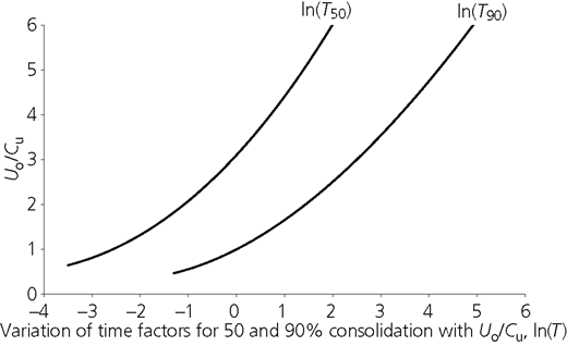
Using an automated process does rule out the possibility of one simple error – misreading the graph. Two of the examples given in the Clarke et al. (1979) paper suffer from this, although that does not detract from the importance of the concept.
The next attempt at making the analysis easier was by treating the decay as exponential. It is not exponential, but may be made to appear so by suitable adjustment of the residual pressure. Plotting the logarithm of the excess pressure against time gives a straight line, after an initial steeper portion. The half-life from the straight line may be used in place of t50, while the residual pressure helps define Uo. This is particularly useful when analysing the decay in total pressure, where the theoretical basis for the residual pressure is less clear.
Note that the use of the ‘half-life’ overestimates t50 because it ignores the initial steeper part of the decay; it therefore underestimates CH. The amount by which this happens increases as the consolidation increases. The method does have its uses, however, as it is often still possible to fit a straight line to noisy data. It also does not rely on the decay reaching 50%.
In all these methods, the decay of the total pressure is treated in exactly the same manner as the pore pressure, but sometimes gives very different results. It is also noticeable that the total pressure is much more sensitive to changes in the expansion. More on this later.
The piezocone and the dilatometer test
Both these devices may be used to monitor the decay of pore water pressures after insertion. Both have the advantage that the expansion cannot change. The piezocone measures the pore water pressures directly and may be left for long periods to monitor the complete decay. The pressure is normally plotted against log t, and t50 is used to estimate CH. This is usually done using a chart, as described by Robertson et al. (1992). Note that the rigidity index, IR (= G/Cu), must be estimated, and the same graphical uncertainties apply. The result obtained can only be an approximation. Some versions of this chart include a plot against √t – this will be returned to later.
The dilatometer test (DMT) allows measurements related to total pressure and pore pressure – the former from the pressure at which initial movement occurs (point A) and the latter from final closure (point C). Both give similar plots to the piezocone against log t, but to speed up the procedure, the point of maximum slope is used. From here to the consolidation is largely empirical, due to the non-cylindrical shape of the blade.
Deriving permeability from consolidation
The theory of vertical consolidation is described by Terzaghi and introduces the coefficient of consolidation – CV, defined by the equation
where k is the coefficient of permeability (or hydraulic conductivity), mv is the volume compressibility and γw is the unit weight of water.
Now, volume compressibility is normally the inverse of bulk modulus, but here the compression is one dimensional and it would appear that the modulus Ev (the constrained modulus) is appropriate to this mode of deformation
where ν is Poisson’s ratio.
Now
Combining Equations 7 and 8 gives
which gives
so defining C in terms of k and G.
The normal requirement is to estimate the permeability from the consolidation
= C/G × 1·166 × 10−10 m/s if C is in square metres/year, G is in megapascals and ν is assumed to be 0·2 – the user may choose another value, but this has invariably been specified in the past.
Simulating the decay
The software used was designed to examine what happens during a constant-flow-rate permeameter test and in particular to test the validity of ‘turboing’ or using high flow rates to move rapidly from one steady state to the next. (See the paper by Ratnam et al. (2005) for a full description of the test.)
It consists of two interlinked spreadsheets, representing the pressure and flow of water radially out from the probe. Changes in pressure affect the flow, and changes in flow affect the pressure. The setting of suitable boundary conditions allows modelling of the holding test, with the ability to change the input parameters at will. The parameters used are
k: the coefficient of permeability
Ev: the ‘bulk’ modulus (connected to the shear modulus G by Poisson’s ratio)
Cu: the shear strength
Uo: the maximum pore pressure generated
ro: the radius of the expanded probe.
Note the use of Ev, the constrained modulus for the bulk modulus – the same argument applies as used earlier.
The two major assumptions are that all flow is radial and that the permeability is constant (although this could be varied if so wished). The underlying theory is that the soil and water behave in accordance with purely physical laws – no soil mechanics is involved.
The first thing to be seen is that the pressure reduction with radius given by Equation 2 results in a constant outwards flow. This is, perhaps, not unexpected, but does inspire confidence in the model. A number of relationships may be found.
(a) t50 is inversely proportional to kEv.
(b) t50 is proportional to .
(c) t50 is approximately proportional to (Uo/Cu)2.
(d) On the plot of pressure against ln t, the maximum slope occurs close to t50 (thus validating the DMT approach).
(e) This maximum slope (Smax) depends only on Uo. The value of Smax is approximately equal to Uo/5.
Looking at the plot against √t shows that the initial part is indeed a straight line. If the slope of this is called So
(f) So is proportional to (kEv)1/2.
(g) So is proportional to Cu.
(h) So is inversely proportional to ro.
(i) So is independent of Uo, which appears a little surprising, until Equation 4 is looked back at.
The product ‘kEv’ is, as has been shown in the section headed ‘The piezocone and the dilatometer test’, closely related to CH. In fact, the two are proportional, and CH may be substituted for kEv in relationships (a) and (f).
So relationships (a), (b) and (c) may be combined into one equation
or
where A is a constant.
Compare this with Equation 5
or
from which it can be seen that
In practice, the following relationship is used
Similarly relationships (f), (g) and (h) may be combined
where B is a constant.
It was noted in the section headed ‘The piezocone and the dilatometer test’ that the piezocone chart often includes the √t plot. An analytical solution derived by Teh (1987) for the piezocone gives
where M is a constant and m is the slope of the plot, using normalised pressures – that is
The only difference between Equations 18 and 20 is the expression (IR)1/2/[ln(IR)]2. This turns out to be almost constant over the range of IR from 10 to 500.
Some practical examples
The following worked examples show various methods of analysis applied to one particular test in London clay (Figure 2).
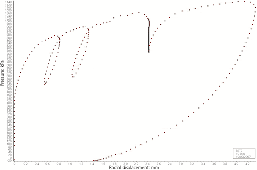
As can be seen, the expansion is held constant at approximately 2·4 mm, which added to the initial radius of the probe of 44·5 mm gives an expanded radius of 46·9 mm.
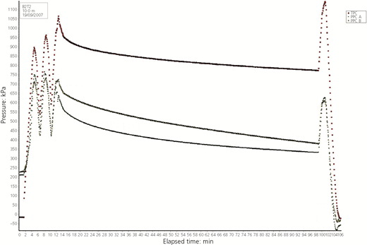
For those with no knowledge of the Cambridge Insitu SBPM, it contains three pressure measuring cells – a total pressure cell (TPC) for measuring the internal gas pressure and two pore pressure cells (PPC A and PPC B) for measuring the external pore water pressure on opposite sides of the membrane. Note that the TPC output displayed has been corrected for the pressure required to expand the membrane (Figure 3).
The test is 10 m below ground level, and the water table is at about 2·5 m, so the ambient water pressure at the test depth is about 75 kPa. The actual pressure measured by the pore pressure cells after drilling the probe into position is about 220 kPa. The residual, or aiming, pressure for the decay would be expected to be somewhere in this range.
Again, for those with no knowledge of the SBPM, the process of drilling raises the pore water pressures in the surrounding soil. It used to be thought that these should be allowed to decay before starting the test, but now they are treated as being part of it.
The measured maximum pore pressure at the start of the hold is 689 kPa. The calculated increase due to the measured expansion is 463 kPa (see Equation 1), which added to the pressure at the start of the test gives a predicted maximum of about 683 kPa – a reasonably close match.
Two different calculations are possible, one using measured values and the other using those predicted by theory – surprisingly the result is very similar (Table 1).
Results from measured and predicted values
| Parameter | Measured value | Predicted value | Units |
|---|---|---|---|
| Maximum pressure | 689 | 683 | kPa |
| Minimum pressure | 220 | 75 | kPa |
| Uo (max − min) | 469 | 608 | kPa |
| Halfway pressure | 454·5 | 379 | kPa |
| Time to halfway (t50) | 31·6 | 70·7 | min |
| Uo/Cu | 2·35 | 3·05 | |
| ln(T50) | −0·735 | −0·073 | |
| T50 | 0·48 | 0·93 | |
| CH | 17·6 | 15·2 | m2/year |
The change in t50 due to the different minimum pressure is almost exactly compensated for by the change in T50 due to the different value of Uo/Cu. The choice of minimum, or residual, pressure turns out to be much less important than at first thought.
Table 2 shows the results from the half-life method.
Results using the half-life approach
| Parameter | Value | Units |
|---|---|---|
| Maximum pressure | 689 | kPa |
| Minimum pressure | 225 | kPa |
| Uo (max − min) | 464 | kPa |
| Half-life | 68·4 | min |
| Uo/Cu | 2·33 | |
| ln(T50) | −0·761 | |
| T50 | 0·47 | |
| CH | 7·9 | m2/year |
The value of consolidation derived is, as expected, somewhat lower with this method.
The half-life derived from the straight part is longer than the actual time for the pressure to halve, because the initial faster drop is ignored (Figure 4). This is the reason for the lower value for the consolidation. It would be possible to correct this error using a mythical T(half-life) in place of T50, but this has never been pursued.
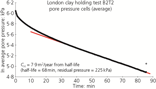
The plot of the log of the excess pressure against time shows a nice straight portion, after the initial fall
The plot of the log of the excess pressure against time shows a nice straight portion, after the initial fall
A similar approach may be used for the total pressure decay, using a mixture of measured and predicted values (Table 3).
Results for total pressure
| Parameter | Measured/predicted | Half-life approach | Units |
|---|---|---|---|
| Maximum pressure | 1096 | 1096 | kPa |
| Minimum pressure | 588 | 700 | kPa |
| Uo (max − min) | 508 | 396 | kPa |
| Halfway pressure | 842 | — | kPa |
| t50 or half-life | 27·6 | 62·1 | min |
| Uo/Cu | 2·54 | 1·98 | |
| ln(T50) | −0·538 | −1·143 | |
| T50 | 0·58 | 0·32 | |
| CH | 24·5 | 5·9 | m2/year |
These results show more variation than those from the pore pressure decay, possibly due to the total pressure being more sensitive than the pore pressure to changes in the strain. In this test, the strain overshoots, drops and then slowly increases again – this will have the effect of increasing the pressure drop at the start of the hold and decreasing the rate of fall towards the end.
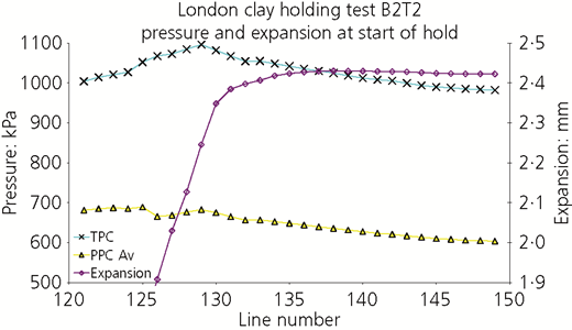
The two problems of deciding on the maximum pressure and exactly when the hold starts are often connected. It is not possible to stop the expansion of the pressure instantly, and, as happens in the example here, there is often an overshoot at the start (Figure 5).
Use of the plot of pressure against the square root of the time (Figure 6) can help here – projecting the straight line drawn through the initial part, back to zero time gives a value for pressure at start of hold (Pmax). It is immediately apparent that the initial overshoot does not fit the rest of the curve – ignoring it gives lower values than used previously.
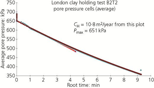
The variation due to the choice of start time turns out to be very small; the reduction in Pmax from ignoring the initial overshoot has a bigger effect, but even this is not really significant.
Effect of choosing different start times for high minimum pressure
| Parameter | Case 1 | Case 2 | Case 3 | Units |
|---|---|---|---|---|
| Start line | 123 | 129 | 135 | |
| Maximum pressure | 670 | 660 | 651 | kPa |
| Minimum pressure | 220 | 220 | 220 | kPa |
| Uo (max − min) | 450 | 440 | 431 | kPa |
| Halfway pressure | 445 | 440 | 435·5 | kPa |
| Time to halfway (t50) | 36·6 | 38·2 | 39·4 | min |
| Uo/Cu | 2·26 | 2·21 | 2·16 | |
| ln(T50) | −0·836 | −0·890 | −0·940 | |
| T50 | 0·43 | 0·41 | 0·39 | |
| CH | 13·7 | 12·4 | 11·5 | m2/year |
Effect of choosing different start times for low minimum pressure
| Parameter | Case 4 | Case 5 | Case 6 | Units |
|---|---|---|---|---|
| Start line | 123 | 129 | 135 | |
| Maximum pressure | 670 | 660 | 651 | kPa |
| Minimum pressure | 75 | 75 | 75 | kPa |
| Uo (max − min) | 595 | 585 | 576 | kPa |
| Halfway pressure | 372·5 | 367·5 | 363 | kPa |
| Time to halfway (t50) | 76·4 | 79·0 | 82·0 | min |
| Uo/Cu | 2·98 | 2·93 | 2·89 | |
| ln(T50) | −0·130 | −0·175 | −0·216 | |
| T50 | 0·88 | 0·84 | 0·81 | |
| CH | 13·3 | 12·3 | 11·4 | m2/year |
In fact, none of the possible problems mentioned earlier seems to have any significant effect on the result, apart from the flawed half-life method. The conversion from consolidation to permeability harbours more potential errors, due to having to estimate Poisson’s ratio. The simulation does not help here, as, although the permeability is entered directly, it still relies on Poisson’s ratio to convert shear modulus to bulk modulus. A value of 12 m2/year gives a permeability of 0·7 × 10−10 m/s for this material (from Equation 11).
As described in the section headed ‘Simulating the decay’, the initial slope of the √t plot gives the permeability directly. This can be useful if the hold is cut short for any reason. All that is required is a value for the constant ‘B’ in Equation 18
The simulation gives a value for B of 2·74 if r is in millimetres and the time in minutes, which for the example shown gives CH = 11·7 m2/year. The same approach for the total pressure gives CH = 18 m2/year, but there is no clear straight-line portion on this plot. One problem is that these results do vary quite widely with the choice of start time, so this method is not recommended for general use. It does, however, allow for the use of much shorter holds.
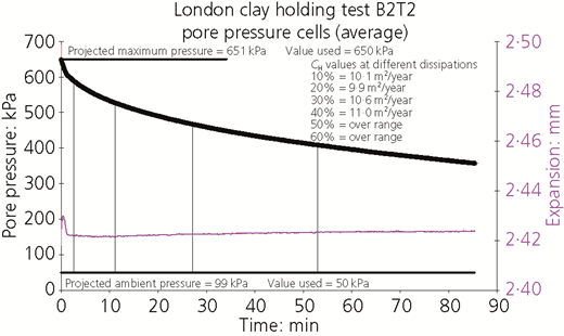
Having a working simulation of the decay allows the time factors to be calculated for other dissipations, besides the previous 50 and 90%. This may be used to give a series of results, which should be identical. Figure 7 shows an example of this method. The problem here is that a curve-fitting technique must be used to match the test curve.
How now can the simulation improve on the results already obtained? The answer would seem to be by a system of curve-matching, producing the best overall match for all the plots discussed with a single value of consolidation and permeability (Figure 8).
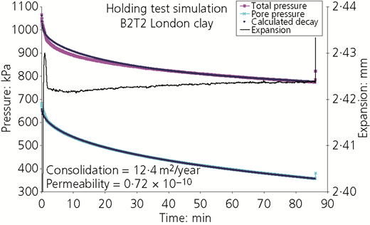
A good match may be achieved for the PPC plot, but the problem is the TPC plot, which is more affected by the changes in expansion, making a good match more difficult.
The answer is to include, in the simulation, compensation for the changes in expansion (Figure 9).
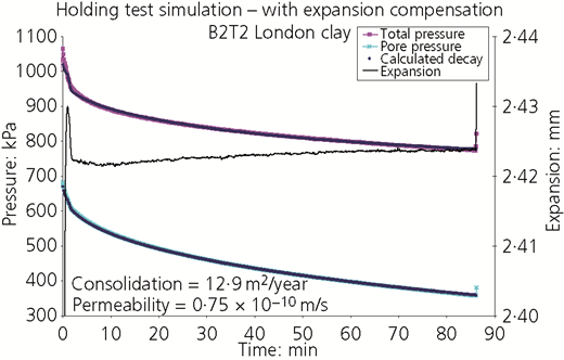
One problem with this is that, for the first time, soil mechanics has become involved in the simulation! The other, more practical problem is that the time bases of the simulation and the original test have to be the same to allow the compensation to be applied. All this is unnecessary if the original hold is good enough.
On a final note, it is possible to simulate the ‘pressure hold’, but it involves the use of a ‘goal-seeking’ add-in along with the expansion compensation used here.
Conclusions
It has been shown that the pressuremeter strain holding and the piezocone dissipation test are closely related and may be analysed mathematically, giving an increase in accuracy over the previous graphical methods. A computer simulation of the decay of pore water pressures, using an Excel spreadsheet, allows a study of the way that this decay depends on various soil parameters. It also leads to a new method of analysis by matching the computer-generated curve to the test curve.
A demonstration of the various methods of analysis applied to one particular test shows that they all give similar results, and many of the uncertainties are not as important as first thought. Anybody seriously interested in the best result will use as many as possible of the methods described.
One possibility for the future is the application of the method to probes that lack pore pressure measurement – reliable results may be obtained from the total pressure alone.

