


The response of gravity retaining walls under strong earthquake motions is a topic of concern since large catastrophic failures have become more frequent during earthquake and post-earthquake events. Neglecting the amplification of ground motion along the surface was an important reason for severe damages in the 1985 Mexico City earthquake and the 1989 Loma Prieta earthquake. In this paper, the response of a gravity retaining wall under different earthquake motions is analysed using a two-dimensional finite-difference method. The strong-motion parameters, peak ground acceleration (PGA) and predominant frequency are particularly investigated. The responses of the retaining wall in terms of the relative horizontal displacement of the wall, active pressure on the wall and response spectra are analysed for input motions with varying PGA and predominant frequency. An empirical equation for the amplification factor at the top of the wall is developed as a function of the PGA and predominant frequency from the observed results. Such an equation can be particularly helpful for rapid assessments of gravity retaining walls in terms of their earthquake resilience and can be assimilated within the design process with relative ease.
Notation
- A
amplification factor
- amax
peak ground acceleration of motion
- e
void ratio
- f
frequency of motion
- f0
natural frequency of motion
- fmax
maximum frequency of motion
- fn
natural frequency of the soil
- G
shear modulus of soil
- g
acceleration due to gravity
- H
thickness of the soil layer
- K
bulk modulus of the soil
- kn
normal stiffness of the zone
- n
mode number
- vs
shear wave velocity of the soil
average shear wave velocity of the soil
- Δzmin
width of the smallest adjoining zone
- σm
mean confining stress
- υ
Poisson’s ratio
Introduction
The failure of retaining walls due to excessive displacement has been observed from previous earthquake events (Carlton et al., 2016; Fang et al., 2003). In several instances, even after ensuring a sufficient factor of safety against sliding, overturning and the overall stability of the surrounding soil, visible damages were observed to the wall after an earthquake. Soil condition has been reported as the primary cause of such failures (Andrianopoulos et al., 2016; Faccioli et al., 2002; Nath et al., 2005; Sandhu et al., 2020). The 1985 Mexico City earthquake (Ashford et al., 2000; Chávez-García and Bard, 1994; Garini et al., 2020; Verde, 1991), the Loma Prieta earthquake in 1989 (Boatwright et al., 1991; Seekins and Boatwright, 1994), the Northridge earthquake in 1994 (Field et al., 1997; Trifunac and Todorovska, 2000) and the Bhuj earthquake in 2001 (Chopra et al., 2013; Sitharam and Govindaraju, 2004) are a few examples of such extensive destruction due to the amplification of ground motion. The high consequences of potential failure during an earthquake emphasise the prominence of the seismic design of retaining walls. The extensively popular pseudo-static Mononobe–Okabe method (Mononobe and Matsuo, 1929; Okabe, 1924) converts the seismic load into equivalent static loads by introducing vertical and horizontal seismic coefficients. Despite its popularity, this method is limited by its assumptions, which neglect dynamic soil properties, wall inertia, amplification and resonant characteristics of soil (Rajesh and Choudhury, 2017). The design is based on the criterion of no displacement, which implies that the dimension of the wall should be large enough to prevent any displacement. An appreciable movement, on the other hand, can lead to significant construction and operational cost of the structure.
The amplification of seismic motion, as the wave approaches the ground surface, is an important factor to be considered in the design. The amplification factor (Kramer, 1996; Panzera et al., 2013), defined as the ratio of the peak ground acceleration (PGA) experienced at any soil depth to the PGA of the base motion (Falcone et al., 2020; Suetomi et al., 2004), should be predetermined before the seismic design to incorporate safely the additional factor of safety. Several factors influence the amplification characteristics, including non-linear soil behaviour, presence of shallow sediments and soil, ground motion characteristics and wall properties (Moschetti et al., 2019; Zaslavsky and Shapira, 2000). The site effects and the direction of maximum surface wave radiation strongly amplify the ground motion (Alvarado et al., 2020; Kumar et al., 2015; Veletsos and Prasad, 1989). The non-linearity of soft soil behaviour significantly influences the amplification factor for seismic accelerations over a PGA of 0.1g. The influence of the saturation states of the soil layer on the amplification of motion as well as the amplification ratio in the vertical and horizontal directions was studied by Yang (2006a). A change in the saturation level from fully saturated to partially saturated was observed to cause significant influence on the vertical acceleration but only a negligible influence on the horizontal acceleration. Although many studies are available on amplification of ground motion (El-Hussain et al., 2013; Fandi and Alyazjeen, 2011, 2013; Garini et al., 2015; Majdeddin et al., 2012; Rahman et al., 2012), only a few studies have focused on the quantification of the amplification factor. Eurocode 8 (BSI, 2004a, 2004b) accounts for the influence of local site conditions by introducing the PGA-normalised response spectra and the soil factor, which represents ground motion amplification with respect to outcrop conditions. The shear wave velocity up to the upper 30 m soil profile, Vs,30, is the main parameter used along with the standard penetration test blow count and shear strength of the soil for the site classification. Even though Vs,30 can be easily determined, knowledge of the Vs profile at the upper 30 m cannot quantify properly the effects of the real impedance contrast, which is one of the main sources of the soil amplification (Firat et al., 2016). Consequently, other parameters of soil characteristics and earthquake motion should be studied to find the correlation to determine the amplification factor. The influence of PGA and frequency of motion on the amplification factor is observed in many studies. Zaslavsky et al. (2003) reported that an amplification effect of a factor of 3–6 is observed within a frequency band of 0.8–6.0 Hz. The mainshock and aftershock accelerograms from the sites recorded amplification factors as high as 10 in the Marina district of San Francisco (Boatwright et al., 1991). The ground motion amplification by a factor of 2 was observed for the mainshock of the Northridge earthquake in 1994 (Paoloucci, 2002). A soil amplification of 2 was reported for the 1979 Coyote Lake earthquakes, with a PGA of 0.26g, and factors of 2 and 0.75 for the 1984 Morgan Hill and the Loma Prieta earthquake, with PGAs of 0.1g and 0.35g, respectively (Beresnev and Wen, 1996). Wang et al. (2018) reported the frequency dependency of topographical amplification. The maximum topographical amplification ranged from 1.6 to 2.0 in the protruded areas. The amplification of PGA tends to reduce as the input motion amplitude increases (Paoloucci, 2002). Martirosyan et al. (2003) summarised that ground motions below 2 Hz have no significant effect on the amplification of motion; however, above 2–3 Hz, the amplification values are greatly reduced. While the amplification of ground motion is a well-addressed topic, the amplification of ground motion along the backfill of a gravity retaining wall has not been studied yet. Such a study not only enables engineers to carry out designs rapidly but also helps in assessments, particularly when such infrastructure assets are affected by climate or anthropogenic hazards. Computationally inexpensive estimates for such amplification can also provide inputs towards resilience, maintenance and intervention ideas for the built infrastructure network (Wenzel and Pakrashi, 2019), including guidance towards inspection and value of information (Quirk et al., 2018), instrumentation and eventual model updating or even digital twinning, as has been observed in cognate areas of research (Buckley et al., 2018). With a rapid evolution of structural assessment in the recent times, this provides a timely insight into this amplification in a reasonable manner. A typical gravity retaining wall is considered in this regard to understand the amplification of motion behind the wall. Studies considering the amplification characteristics of cohesionless soil beneath and behind a gravity retaining wall are limited in the literature. The influence of PGA and frequency of motion on the amplification factor is observed in many studies, but the quantification of the amplification factor as a combination of PGA and frequency of motion is not addressed yet. The present study is extended to develop an empirical equation of the amplification factor at the top of the wall that can be readily used by engineers to consider preliminary estimates or rapid assessments of the displacement of the wall, particularly when extensive numerical modelling is not possible. The variation of the amplification factor along the retaining wall depth is a topic of interest undertaken in the present study.
In this paper, a numerical study on a gravity retaining wall is conducted to study the effect of the amplification of strong motion on the wall response under earthquake motions of acceleration time histories by varying the PGA from 0.16g to 0.36g. The influence of strong-motion parameters such as PGA and predominant frequency is extensively studied. The impact of amplification of ground motion is investigated, and a significant influence of amplification on the displacement of the wall is established. To aid future design and assessment processes, including rapid implementation of such estimates without the requirement of extensive computing, an empirical equation is developed from the numerical results for the amplification factor at the top of the wall as a function of PGA and predominant frequency of motion. Such an empirical relationship will be of relevance to both practitioners and researchers while creating a pathway for future assimilation of such an approach to normative documents.
Description of the model
Problem definition
A retaining wall model was analysed for evaluating the amplification characteristics of input motion and the permanent displacement of the wall during different seismic events. Typically, a wide range of materials is used as backfill material, including clean granular soil free of frozen lumps, organic matter, trash, chunks of highly plastic clay, snow, ice or any other objectionable material (Patki et al., 2015; Yang and Tang, 2017). A gravity retaining wall holding a dense cohesionless backfill soil was chosen for the numerical study, modelled using the finite-difference software FLAC 7.0 (de Lemos, 2012; Detournay and Hart, 2020) and validated with results from the existing literature (Deyanova et al., 2016). The gravity wall model was subjected to acceleration time histories of real earthquake records. The PGA and the predominant frequency of motion were extensively investigated through numerical analysis to understand their influence on the response of the wall. The acceleration time histories, response spectra and the horizontal permanent displacement of the wall were analysed at every 1 m depth along with the wall height. The influence of PGA and predominant frequency of motion was subsequently studied by applying ground motions of PGA varying from 0.16g to 0.36g and predominant frequency ranging 0.3–5.0 Hz. This led to an empirical formulation for calculating the amplification of ground motion at the ground surface based on PGA, frequency of motion and natural frequency of soil.
Wall geometry and soil properties
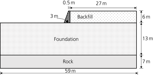
The gravity retaining wall was trapezoidal (0.5 m top width, 3 m bottom width, 6 m height) and made of concrete; it was modelled with dense foundation and backfill soil of density 2000 kg/m3 adopted from the paper by Deyanova et al. (2016), as presented in Figure 1. The retaining wall rests on foundation soil of depth 13 m, overlying rock of 7 m thickness. The properties specified in Table 1 were assigned to the soil and wall. The Mohr–Coulomb failure criterion with non-linear hysteretic and Rayleigh damping was considered for the soil (Esqueda and Botello, 2005; Madabhushi and Zeng, 2007; Salman et al., 2010), while the foundation depth and side dimensions prevented any boundary effects. The Mohr–Coulomb failure criterion characterised by a shear yield function with tension cut-off, a non-associative flow rule for shear failure and an associative flow rule for tension failure was adopted for the present study. This failure criterion when coupled with cyclic loading developed rate-independent hysteretic damping causing energy dissipation within the soil. An additional Rayleigh viscous damping captured the soil damping at very low strains. This strain-dependent soil behaviour was set active throughout both the static and dynamic analyses. The non-linear backfill and foundation soil properties were modelled with a shear modulus degradation curve considered as per the thesis by Darendeli (2001). The shear modulus and bulk modulus of the soil were calculated following Ishihara (1996) as per
where K and G are the bulk modulus and shear modulus of the soil, respectively; e and υ are the void ratio and Poisson’s ratio of the soil, respectively; and σ m is the mean confining stress. The soil layers were divided into sub-layers of 1 m depth with constant geotechnical properties within their thickness. The retaining wall and the rock base were modelled as linear elastic (Deyanova et al., 2016; Ibrahim, 2015). The properties of soil and retaining wall used are given in Table 1.
Soil and wall properties
| Soil type | Backfill | Wall | Base |
|---|---|---|---|
| Void ratio | 0.45 | — | — |
| Mass density: kg/m3 | 2000 | 2400 | 2400 |
| Friction angle: ° | 37.5 | — | — |
| Dilation angle: ° | 5 | — | — |
| Shear modulus: MPa | 2.20 × 10⁹ | 2.00 × 10⁹ | |
| Cohesion: MPa | 0 | — | — |
| Poisson’s ratio | 0.3 | 0.2 | 0.29 |
| Model | Non-linear hysteretic + Mohr–Coulomb failure criterion + viscous damping | Linear elastic | |
Selection of earthquake data
The acceleration time histories of seven different earthquakes (Bhuj (2001), Nepal (2015), Myanmar (2016), Tabas (1978), Kyushu (2005), Kobe (1995) and Izmit (1999)), as presented in Table 2, were used for numerical analysis following baseline correction of excitation data and filtering of noises (Gupta and Trifunac, 2017; Zhou et al., 2020). The corrected acceleration time histories were scaled to match with the target spectra of PGAs of 0.16g, 0.24g, 0.28g and 0.36g, respectively, to achieve spectrum compatibility so that the difference between the target spectrum and the average spectrum was less than 30% within a period of 0.05–2.00 s. Eurocode 8 (BSI, 2004a, 2004b) was adopted for choosing the design target spectrum, which is an elastic acceleration response spectrum at 5% structural damping on type 1 rock.
Input ground motion
| Record | Earthquake | Station | Magnitude, Mw | PGA: g | Scaling factor | Scaled PGA | Predominant frequency |
|---|---|---|---|---|---|---|---|
| A1 | Bhuj/Kachchh, 2001 | Ahmedabad, India | 7.6 | 0.106 | 2.69 | 0.285 | 5 |
| A2 | Lamjung, Nepal, 2015 | Kanti Path, Kathmandu | 7.8 | 0.158 | 2.22 | 0.35 | 0.31 |
| A3 | Myanmar, 2016 | Haka, Myanmar | 6.8 | 0.084 | 3.33 | 0.28 | 4.54 |
| A4 | Tabas, Iran, 1978 | Dayhook | 7.3 | 0.373 | 0.754 | 0.281 | 3.33 |
| A5 | Kyushu, Japan, 2005 | Chinzei, Japan | 6.6 | 0.144 | 2.02 | 0.291 | 3.33 |
| A6 | Kobe, Japan, 1995 | Nishi-Akashi | 6.9 | 0.509 | 0.638 | 0.325 | 4.54 |
| A7 | Izmit, Turkey, 1999 | Ambarli-Termik Santrali | 7.6 | 0.253 | 1.2 | 0.30 | 2.78 |
Interface and boundary conditions
The two-dimensional numerical model of a retaining wall in Figure 1 was developed using the FLAC 7.0 software. The meshing of the model (see Figure 2) was provided using square grid zones of size 0.5 m closer to the retaining wall and 1 m for faraway zones. The zone size was selected to allow the propagation of input waves of maximum frequency (Kuhlemeyer and Lysmer, 1973) calculated as
where f max is the maximum frequency that can be modelled, which for the present study is assumed as 10 Hz. Δl is the minimum size of mesh required in the analysis. Interface elements were used to define the boundaries between soil and wall, which ensured the transfer of complete pressure field while enforcing geometric compatibility. The interface properties shear (k s) and normal stiffness (k n) were assigned to the interface elements along with the interface friction angle calculated (Itasca, 2011) as
where K, G and Δz min are the bulk modulus, shear modulus and the width of the smallest adjoining zone in the normal direction, respectively. The normal stiffness and shear stiffness were chosen to be equal for the analysis. The Lysmer and Kuhlemeyer (1969) absorbing boundary of independent viscous dashpots placed vertically and horizontally at the boundaries was adopted in the present analysis. The free-field boundary applied at both vertical boundaries absorbed the outward wave propagation and preserved the non-reflecting properties. It also helped in minimising the distance towards the boundary away from the structure, which could be numerically expensive.
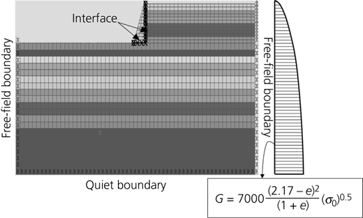
Generated mesh of the gravity retaining wall and shear modulus variation with depth
Generated mesh of the gravity retaining wall and shear modulus variation with depth
In the first phase of the numerical analysis, static equilibrium was established by bringing the unbalanced force approaching zero. Subsequently, dynamic analyses were carried out by applying earthquake excitations (see Table 2) to the base of the model and propagated upwards. Hysteretic damping was applied to the model based on the shear modulus decaying curve following the paper by Deyanova et al. (2016). An additional Rayleigh viscous damping of 0.1% was provided to capture soil damping at very low strains. Before the numerical study, the model was validated against the paper by Deyanova et al. (2016). Subsequently, the influence of PGA and predominant frequency on the amplification characteristics was studied separately and combined, following the establishment of an empirical equation for the amplification factor at the top of the wall.
Validation of the model
The numerical model was then validated against the paper by Deyanova et al. (2016). For the validation, Tabas (1978), Loma Prieta (1989) and Kyushu (2005) earthquake data (see Table 3) were used. The corrected acceleration time histories, used as base excitations, were matched with a 0.28g target spectrum as per Eurocode 8 (BSI, 2004a, 2004b) within the period range 0.15–2.00 s so that the difference between the average spectrum and the target spectrum did not exceed 10%.
Input ground motion for validation of the model
| Record | Earthquake | Station | Magnitude, Mw | PGA: g | Scaling factor | Scaled PGA | Predominant frequency |
|---|---|---|---|---|---|---|---|
| 1 | Tabas, Iran, 1978 | Dayhook | 7.3 | 0.373 | 1.1 | 0.412 | 0.16 |
| 2 | Loma Prieta, California, USA, 1989 | Gilory Array #1 | 6.9 | 0.442 | 0.403 | 0.178 | 0.38 |
| 3 | Kyushu, Japan, 2005 | Chinzei, Japan | 6.6 | 0.141 | 2 | 0.282 | 0.08 |
The relative horizontal displacement at the bottom of the wall, defined as the difference between the horizontal displacement of the wall and the free-field horizontal displacement, along with the tilt of the wall and the ground settlement behind the wall was estimated next from the analysis. The tilt of the wall is defined as the ratio of the difference between the horizontal displacements at the top and bottom of the wall to the wall height. The horizontal displacement at the bottom of the wall was compared against the results of Deyanova et al. (2016) in Figure 3. It was observed that despite uncertainties in soil properties, the horizontal displacement as computed from the present analysis matched favourably with that reported by Deyanova et al. (2016). The displacement of the wall in the present study shows an average of 10.5% difference in the displacement of the wall under the Tabas (1978) earthquake, while the displacement of the wall under the Kyushu (2005) earthquake show an average of 17.7% underprediction. However, the displacement of the wall under the Loma Prieta (1978) earthquake in the present study shows 2.7% underprediction.
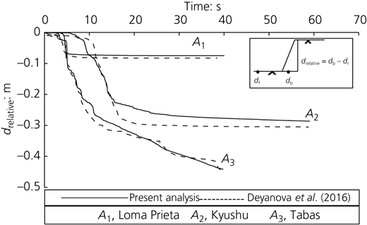
Comparison of the results of the relative horizontal displacement at the bottom of the wall under the Kyushu (2005), Loma Prieta (1989) and Tabas (1978) earthquakes from the present study with the results of Deyanova et al. (2016)
Comparison of the results of the relative horizontal displacement at the bottom of the wall under the Kyushu (2005), Loma Prieta (1989) and Tabas (1978) earthquakes from the present study with the results of Deyanova et al. (2016)
The failure of a retaining wall is not a well-defined criterion. However, it can be defined based on the serviceability criteria or based on any design conditions to be followed. Wu and Prakash (1996) suggested that the horizontal displacement corresponds to failure as 0.1H, where H is the height of the retaining wall, which is followed here. The failure of the wall can be defined through the separate mechanisms of tilting caused by excessive settlement at the base of wall toe and the exceedance of the horizontal displacement of the wall above 10% of wall height.
The wall did not fail under all three earthquakes considered since the horizontal displacement of the wall was less than 600 mm. The tilt of the wall was compared with the results of Deyanova et al. (2016) (see Figure 4), and the difference in tilt in both cases was less than 0.01 rad (0.5°).
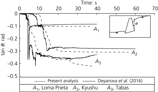
Comparison of the tilts of the wall under the Kyushu (2005), Loma Prieta (1989) and Tabas (1978) earthquakes from the present study with the results of Deyanova et al. (2016)
Comparison of the tilts of the wall under the Kyushu (2005), Loma Prieta (1989) and Tabas (1978) earthquakes from the present study with the results of Deyanova et al. (2016)
The settlement up to 7 m from the wall in the backfill was calculated next. Figure 5 shows that the settlement of backfill soil computed in the present analysis matches reasonably well with that of Deyanova et al. (2016). The settlement of soil behind the wall based on the present model shows an average of 5% error under the Tabas earthquake. However, the settlement behind the wall induced by the Kyushu earthquake and Loma Prieta earthquake based on the present model shows averages of 9.6 and 16% variation with the result of Deyanova et al. (2016), respectively. Overall, the displacement, settlement and tilt of the wall obtained from the present numerical analysis show agreement with the results of Deyanova et al. (2016).
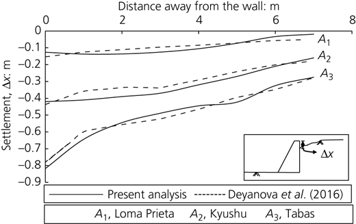
Comparison of the settlement of soil behind the wall under the Kyushu (2005), Loma Prieta (1989) and Tabas (1978) earthquakes from the present study and the results of Deyanova et al. (2016)
Comparison of the settlement of soil behind the wall under the Kyushu (2005), Loma Prieta (1989) and Tabas (1978) earthquakes from the present study and the results of Deyanova et al. (2016)
Numerical analysis of the gravity wall
The earthquake data in Table 2 were matched with target spectra of 0.16g, 0.24g, 0.28g and 0.36g of Eurocode 8 (BSI, 2004a, 2004b) for a parametric study next for a total of 28 different input configurations. The selected PGA and predominant frequencies addressed moderate earthquakes with combinations of both near-field and far-field earthquake conditions. The difference between the matched spectra and the average spectra was allowed an exceedance limit of 30% within a time period of 0.05–2.00 s, which created a small range of PGAs in each case (e.g. acceleration time histories scaled to 0.16g have accelerations of PGAs 0.165g, 0.17g, 0.175g, 0.18g and 0.2g). Overall, different sets of PGA and frequency combinations were used for the study, which helped in understanding the amplification factors for even a small range of variation in PGA. The earthquake motion applied at the base of the model was compared with the predicted acceleration time history for the Bhuj (2001) earthquake under four different PGAs as shown in Figure 6. The graph showed good match between the acceleration time histories applied and the ones predicted in the analysis.
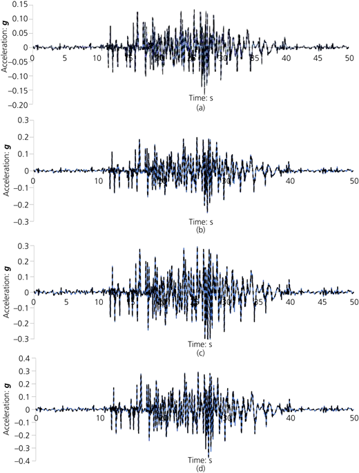
The comparison of input earthquake motion and predicted motion during the Bhuj (2001) earthquake of scaled PGAs: (a) 0.16g, (b) 0.24g, (c) 0.28g and (d) 0.36g
The comparison of input earthquake motion and predicted motion during the Bhuj (2001) earthquake of scaled PGAs: (a) 0.16g, (b) 0.24g, (c) 0.28g and (d) 0.36g
Results and discussion
Response of the gravity wall
The gravity wall model was studied under different earthquake cases, and the relative horizontal displacement of the wall, tilting of the wall, the active pressure on the wall and response spectra at various points were obtained. The relative horizontal displacements of the retaining wall under the given input motions are shown in Figure 7. Failure was assumed to occur at a wall displacement of 60 cm (10% of wall height). However, the permissible displacement of the wall according to the Commission of the European Communities (CEC, 1994) was 300a max, whereas the American Association of State Highway and Transportation Officials (Aashto, 2002) recommended 250a max. Wu and Prakash (1996) suggested the permissible displacement as 0.2 times the height of the wall. Figure 8 shows the deformed mesh of the gravity retaining wall model after being subjected to the Kobe (1995) earthquake. The wall displaced 72 cm for a ground motion of PGA 0.36g and a frequency of 4.5 Hz and hence failed. For the same PGA of ground motion, the displacement varies with the frequency of input motion in a way that as the frequency reduces, the relative displacement at the bottom of the wall increases. In this study, as the frequency was reduced from 4.50 to 3.33 Hz, the relative displacement at the bottom of the wall increased from 8 to 18 cm, whereas for 0.36g motion, the displacement reduced from 72 to 33 cm.
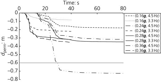
Relative horizontal displacements of the wall under different PGAs and frequencies. The model is analysed for input real earthquake motions of PGA from 0.16g to 0.36g with frequencies 4.5 and 3.3 Hz
Relative horizontal displacements of the wall under different PGAs and frequencies. The model is analysed for input real earthquake motions of PGA from 0.16g to 0.36g with frequencies 4.5 and 3.3 Hz
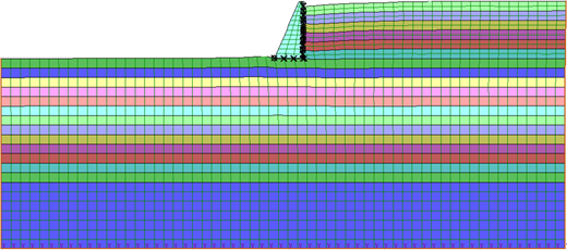
Deformed mesh of the gravity wall model after being subjected to the Kobe (1995) earthquake
Deformed mesh of the gravity wall model after being subjected to the Kobe (1995) earthquake
The response spectra at the bottom of the wall for input motions of PGA 0.16g, 0.24g, 0.28g and 0.36g for frequencies of 5.0, 4.5 and 3.3 Hz are shown in Figures 9(a)–9(c), respectively. From the response spectra of all the aforementioned cases, the maximum response was observed at a period of 0.16 s. The response to the input motion was maximum at 4.5 Hz since the frequency of motion was closer to the natural frequency of the soil (4.23 Hz), which is calculated based on the book by Kramer (1996) as
where is the average shear wave velocity of the soil, H is the thickness of the soil layer and f n is the fundamental frequency at nth mode.
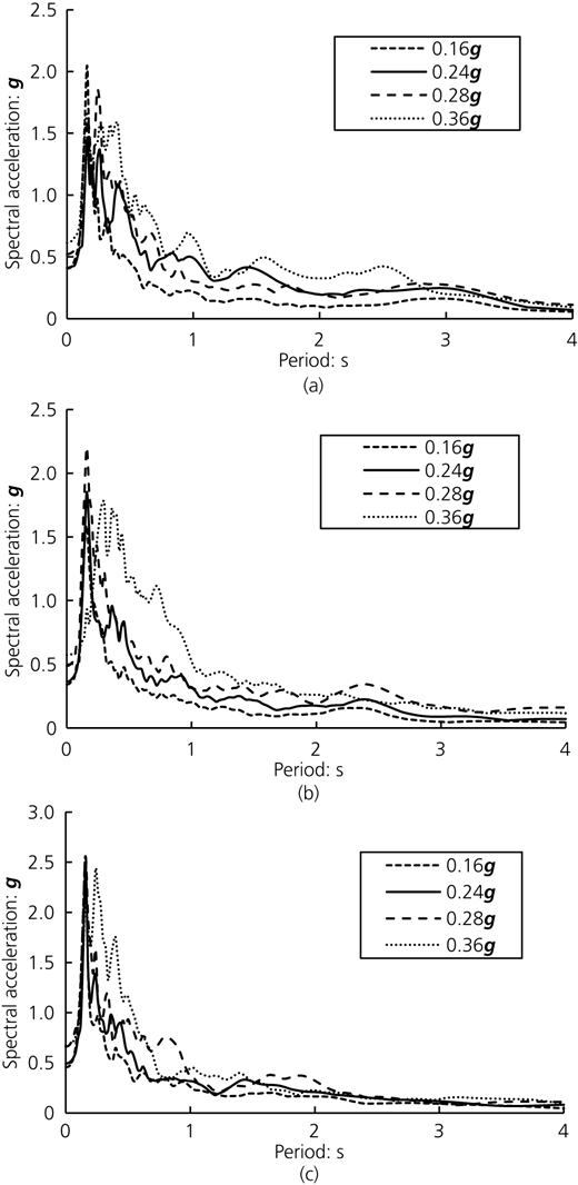
Response spectra at the bottom of the wall for input motions of PGAs 0.16g, 0.24g, 0.28g and 0.36g for frequencies of (a) 5.0, (b) 4.5 and (c) 3.3 Hz
Response spectra at the bottom of the wall for input motions of PGAs 0.16g, 0.24g, 0.28g and 0.36g for frequencies of (a) 5.0, (b) 4.5 and (c) 3.3 Hz
The resonance of ground motion when the frequency of motion is closer to the natural frequency of the ground and natural frequency of the retaining wall was observed, similar to those obtained by Meli et al. (1998). Since the present study was carried out for dry backfill, the total and effective lateral stresses on the wall were the same. The active pressures on the wall for input motions of PGA 0.16g, 0.24g, 0.28g and 0.36g are plotted in Figure 10. The lateral pressure on the wall increased as the PGA of input motion increased from 0.16g to 0.36g. Significant disturbance in the pattern of active pressure distribution was observed as the PGA was increased. The effective stress distribution in the top 1–2 m of soil was not significantly influenced by the varying PGA from 0.16g to 0.36g, unlike those observed in the bottom layers (below 2 m).
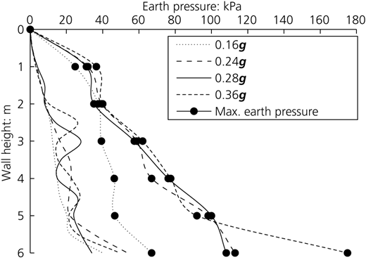
Effective stress on the wall for input motions of PGAs 0.16g, 0.24g, 0.28g and 0.36g. The effective stress at the end of seismic motion, as well as the maximum effective stress during the seismic motion, is shown in the figure
Effective stress on the wall for input motions of PGAs 0.16g, 0.24g, 0.28g and 0.36g. The effective stress at the end of seismic motion, as well as the maximum effective stress during the seismic motion, is shown in the figure
The lateral pressure on the wall at the end of the seismic motion was not the maximum pressure experienced by the wall. As shown in Figure 10, the maximum lateral pressures developed were two to four times higher than the pressure at the end of the seismic event. The maximum lateral pressure on the wall and the maximum wall displacement were observed at the same time with a small phase difference. This phase difference was due to the phase difference of the shear wave propagating in the backfill soil. The lateral pressure on the wall at the end of the dynamic event was observed to be independent of the frequency of the motion, while the maximum lateral pressure developed on the wall was a function of frequency. At lower frequencies, the wall experienced a substantial increase in lateral pressure, which emphasised the fact that the effect of frequency on the dynamic pressure on the wall was as important as the effect of PGA of the motion.
Influence of PGA on amplification
The amplification of ground motion is caused by several factors such as scattering, diffraction and interference of input motion (Lee and Trifunac, 2010; Todorovska and Trifunac, 1997). A better understanding of the ground motion amplification is necessary to know the additional strength demand required for structures that stand over soft soil conditions (Banerjee et al., 2016). The peak ground motion and the frequency of motion are two important factors of earthquake motion influencing most of the phenomenon triggered by the earthquake. In this connection, the amplification of input motion was studied in the present study by analysing the influence of PGA and frequency of motion on the amplification. The amplification of input motion along with the soil depth of the numerical model, under different PGAs, is presented in Figures 11(a)–11(d). The numerical model was analysed under all the seven earthquakes that are matched with the target spectra of 0.16g, 0.24g, 0.28g and 0.36g.
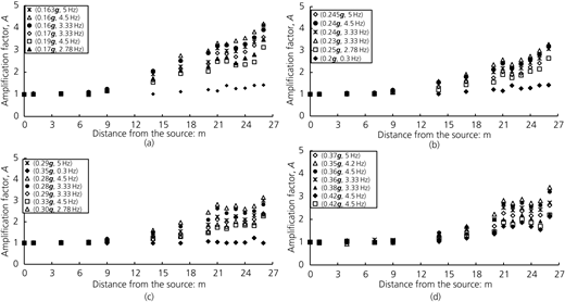
Variation of the amplification factor along with the soil depth under earthquakes matched to target spectra of PGAs: (a) 0.16g, (b) 0.24g, (c) 0.28g and (d) 0.36g
Variation of the amplification factor along with the soil depth under earthquakes matched to target spectra of PGAs: (a) 0.16g, (b) 0.24g, (c) 0.28g and (d) 0.36g
The amplification curve in all cases was nearly horizontal up to 7 m from the base of the model, indicating that the input motion had no significant amplification while passing through the rock. Moreover, the distance from the source (from the point of application of motion in the model) and the characteristics of propagating media were important factors that also influenced the extent of amplification. The amplification of motion was higher as the distance from the source increased due to an increase in scattering and diffraction in the media of propagation (Bard, 1982; Sato et al., 2012). Figure 12 shows that the variation of the amplification factor increases with PGA at the same frequency of motion. It was observed that the amplification factor was higher for lower PGAs and remained constant for higher PGAs (greater than 0.24g). The amplification patterns from the results indicated that the amplification factor reduced as the PGA increased from 0.16g to 0.36g. The amplification factor at the top of the wall was 4.1 for 0.16g and 2.6 for 0.36g. This indicates that factors such as the distance from the source, the PGA, frequency of the motion, backfill and foundation soil properties have a significant influence on the amplification characteristics. Furthermore, a peak in amplification was observed at the top boundary surface as the seismic wave touched the free surface.
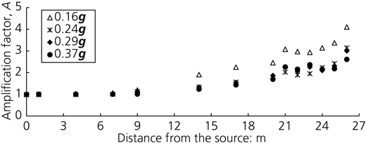
Variation of the amplification factor with PGA at the same frequency of motion
Variation of the amplification factor with PGA at the same frequency of motion
Influence of the frequency of motion on amplification
The frequency of an earthquake has a significant influence on the response of any structure constructed over the soil media as well. Yu et al. (1993) outlined the differences between linear and non-linear responses and marked off three separate frequency bands. The study revealed that the amplification was not significant at lower frequencies but deamplification and amplification of strong motion were observed at intermediate- (1–10 Hz) and higher-frequency bands (greater than 10 Hz). Figures 11(a)–11(d) further show the variation in amplification of motion along with soil depth as the frequency was varied, indicating that the frequency dependency of amplification had a significant impact near the free surface. The amplification factor for 0.16g PGA was 4.1, 4.2, 3.9 and 3.4 at predominant frequencies of 5.00, 4.50, 3.30 and 2.78 Hz. The amplification was almost negligible when the input motion passed through the rock but showed significant variation when passing through the soil. The amplification of motion was higher at a faraway distance from the source, which was like the case of varying PGA. Hence, amplification was higher at the surface, which indicated the necessity of including the amplification factor in the design of the retaining wall. Figures 11(a)–11(d) show that amplification increases as the frequency of motion increases. As the frequency of motion was reduced, the amplification factor was also reduced as the wave was approaching the ground surface. Furthermore, at frequencies less than 1 Hz, the amplification factor approached unity, which indicates that the amplification is insignificant at lower frequencies and need not be considered in design (Yu et al., 1993). These results suggest that while designing retaining walls, an amplification factor corresponding to an intermediate frequency can be adopted for a safer design. Hence, from the analysis, it can be concluded that the amplification of motion is a frequency-dependent phenomenon that increases as the frequency of motion increases and remains constant for higher-frequency motion. In general, the retaining wall sections are designed for base shears and shears at different sections are obtained from the acceleration time histories calculated/measured at the base level. The present analysis suggests that there will be an amplification of the motion at a different level of the retaining walls. The design shear forces, therefore, should be evaluated for the amplified ground motion.
Derivation of the equation for the amplification factor at the wall top
The significance of including the amplification factor in the design is clear from the numerical analysis, as the input wave accelerations were significantly amplified at the ground surface. The amplification of the input wave is influenced by many factors, including backfill and foundation soil properties, magnitude, depth and distance of the specified earthquake and earthquake characteristics. The propagation of earthquake waves while passing through a sufficient thickness of the soil layer results in the filtering of higher frequencies, and the surface of the soil will experience the effect of lower frequencies with longer periods.
Based on the results from the numerical study, an equation for amplification of motion at the top of the wall was developed in this study. While the calibrations around such an equation can change, it is envisaged that the overall form and the range of values will be based on what is developed in this paper. The impact of PGA and the frequency of input motion was considered in the derivation. The dimensionless acceleration represented by the PGA as a fraction of the gravitational acceleration and the frequency ratio defined as the ratio of the predominant frequency of motion to the natural frequency of soil layer are considered the dimensionless quantities in this study. The natural frequency of the soil layer is calculated based on Equation 5.
In Figure 13, the amplification factor at the top of the wall for different sets of varying PGA and frequency of motion are shown. In general, the amplification varies exponentially with the corresponding PGAs. A significant influence of PGA was observed in the amplification factor as the wave propagates towards the ground surface. The amplification of wave at the top of the wall under all 28 sets of earthquake analysis is plotted in Figure 13. Equations 6–8 are derived for a rapid and approximate calculation (within 10% error within the input ground motion acceleration of 0.16g to 0.36g and frequency range of 1–5 Hz) of the amplification factor (A) at the wall top from the results from the present study.
where A is the amplification factor at the top of the wall, f is the frequency of input motion, f 0 is the natural frequency of soil, a max is the PGA and g is the gravitation due to gravity. The equation represents the effect of PGA and frequency on the amplification of motion. Using Equation 6, with known values of the PGA, frequency of motion, natural frequency of ground and flexural rigidity of wall, the amplification of the propagating wave at the wall top can be found. This helps in taking a precaution against the unexpected amplification of motion leading to catastrophic failures as in the case of the Kobe (1995) earthquake (Mylonakis et al., 2006), Athens (1999) earthquake (Bouckovalas and Kouretzis, 2001) and Tohuku (2011) earthquake (Bhattacharya et al., 2011).
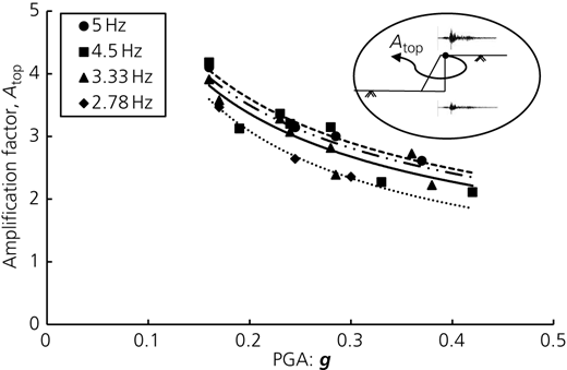
Amplification factor at the top of the wall for different sets of motions with varying PGA and frequency
Amplification factor at the top of the wall for different sets of motions with varying PGA and frequency
The comparison of the amplification factor at the wall top from the derived equation with the results from the numerical study and previous literature is shown in Figure 14. The proposed equation for the amplification factor at the surface was compared with the results by Kumar et al. (2015) and Kristek et al. (2018). Kumar et al. (2015) performed an equivalent linear analysis using the Shake2000 software program to study soil amplification. The soil profile consists of layers of soft soil up to 4–5 m below the overlying stiff soil from 5 to 15 m depth following dense soil at deeper depths. The water table was observed at 0.9 m depth. The amplification factor was compared for the frequency content of the ground motion varying from the lowest value of 2.3 Hz to the highest value of 39.95 Hz, whereas the PGA varied from 0.033g to 0.53g. The developed equation presents an amplification factor lower than that by Kumar et al. (2015). The difference may be due to the variation in soil characteristics adopted in the two studies. Dry cohesionless backfill was used for the present study, whereas silty sand and medium- to low-compressibility clays were considered in the study by Kumar et al. (2015). The degree of saturation has greater influence on the dynamic soil characteristics (small strain modulus, damping and shear wave velocity), which thereby affects the amplification characteristics of soil (Yang and Sato, 2001; Yang, 2006b). Warnana et al. (2012) reported that the amplification in the dry season varied from 2 to 7 and in the wet season varied from 2.6 to 8.3 due to the significant influence of rainfall infiltration. The centrifuge model study by Ghayoomi and McCartney (2012) reported a 20% increase in the amplification factor for partially saturated soil compared with that of soil under dry conditions. Another reason for the difference in the amplification factor is the difference in the ground motion parameter range adopted in the two studies. Figure 14 also indicates that the strong-motion parameters used in the studies by Kumar et al. (2015) and Kristek et al. (2018) are outside the range used in the present study. An average of 59% increase in the amplification factor was reported by Kumar et al. (2015) for ground motions with frequency content ranging 5–39.95 Hz. Hence, the developed equation for amplification factor can be used for ground motions within the varying frequency range 1–5 Hz.
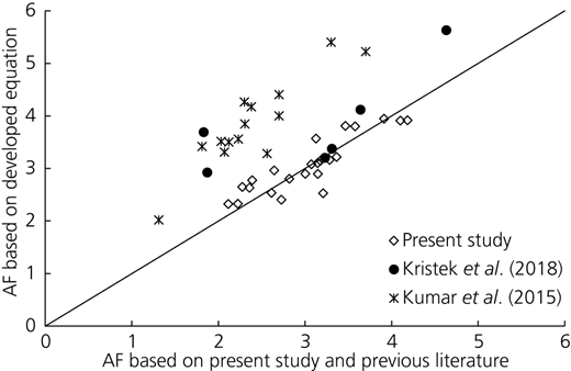
Comparison of the amplification factor (AF) of the wall top from the derived equation with the results from the numerical study and previous literature
Comparison of the amplification factor (AF) of the wall top from the derived equation with the results from the numerical study and previous literature
Kristek et al. (2018) developed a methodology for determining the acceleration and ground motion characteristics using a reference site for two basic configurations. The accelerograms from two receivers (Resource waveform IDs 15537 and 15560) from the Thjorarbru station in two horizontal and one vertical directions during the South Iceland earthquake of 17 June 2000 across the Grenoble valley were used for comparison. The PGA ranges 0.048g to 0.29g, and the predominant frequency ranges 3.3–8 Hz. The amplification factor estimated using the equation developed agrees reasonably with that by Kristek et al. (2018). The amplification factor of ground motion at 0.21g and 3.33 Hz and 0.24g and 3.33 Hz matches equally with the factor estimated with the proposed equation. However, the ground motion of frequency content higher than 5 Hz is on average 48% higher than that of the proposed equation. This indicates that the estimation of the amplification factor using the proposed model is applicable for ground motions within the range of PGA 0.16g to 0.36g and predominant frequency 1–Hz.
Conclusion
The design of retaining walls for the seismic condition is a challenging procedure, as the uncertainties in the design motion parameters and soil properties make the design more complex. The amplification of seismic waves as the waves approach the ground surface is an important reason for large-scale destruction of structures on the surface. This factor is often ignored in the seismic design of retaining walls. In this paper, the authors carry out a numerical study on a gravity retaining wall model subjected to different earthquake conditions. To address the influence of earthquake parameters, the authors subsequently carry out a detailed parametric study involving seven earthquakes on a benchmark example. Subsequently, the authors assimilate these results to develop an equation for the amplification factor at the wall top as a function of PGA and predominant frequency.
The results demonstrate that PGA and predominant frequency of motion impacts on the amplification factor significantly. The frequency of motion influences the relative horizontal displacement of the wall and the active earth pressure on the wall. As the frequency of motion reduced from 4.5 to 3.33 Hz, the relative displacement at the bottom of the wall reduced from 18 to 8 cm, whereas for 0.36g motion, the displacement reduced from 72 to 33 cm. Amplification of ground motion when the frequency of motion reaches close to the natural frequency of ground and the retaining wall was observed in the results. The maximum active earth pressure developed were two to four times higher than the lateral pressure at the end of the seismic event. The active pressure on the wall at the end of the dynamic event was observed to be independent of the frequency of the motion, while the maximum earth pressure developed on the wall was frequency dependent.
The amplification factor increased as the PGA of motion decreased from 0.36g to 0.16g, and the frequency increased from 2.78 to 5.00 Hz. The results from the numerical analysis prove that the PGA and frequency of motion of input motion has a significant influence on the amplification of motion. In the present study, as the PGA increased from 0.16g to 0.36g, the amplification factor reduced from 4.1 to 2.6. Moreover, as the frequency of motion increased from 2.78 to 5.00 Hz, the amplification factor increased from 3.4 to 4.2. The combined effect of PGA and predominant frequency shows some trend in distribution on the amplification behaviour.
The comparison of the proposed equation for the amplification factor at the top of the wall with the previous literature indicates that the proposed equation holds good for ground motions of PGA ranging 0.16g to 0.36g and predominant frequency ranging 1–5 Hz. The analysis and the developed empirical relationship will help engineers consider preliminary estimates or rapid assessments of displacement of the wall, particularly when extensive numerical modelling is not possible. Such work can also be particularly helpful in post-disaster assessments and climate-aware resilience of infrastructure networks. Further study is needed to explore the influence of different backfill and soil conditions on the amplification characteristics.
Acknowledgements
Vikram Pakrashi would like to acknowledge the EU-funded Strengthening Infrastructure Risk Management in the Atlantic Area project (Grant EAPA\_826/2018) and the support of SFI MaREI Centre, UCD Centre for Mechanics and UCD Energy Institute.

