Emergency relief supply chain design and trade-off analysis

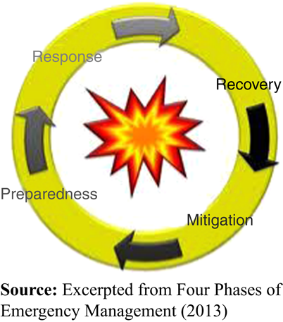
Emergency management (or disaster management) is the discipline of avoiding, mitigating, and managing risks (Haddow et al., 2011). It is also a discipline to prepare for disasters before they happen, responding to them immediately, supporting, and reconstructing the affected areas after disasters have occurred. The disaster management continuum model (Dangi et al., 2012) usually classifies the relevant emergency management activities into a continuous cycle of the four phases of Preparedness, Response, Recovery, and Mitigation. Figure 1 illustrates the cycle of these four phases, followed by the brief explanation of each phase based on the description of Emergency Management and Homeland Security Office Website at City of Providence, RI (Four Phases of Emergency Management (2013)).

Mitigation refers to all activities to reduce the damage and loss from natural and/or man-made disasters by avoiding or alleviating the impact of a disaster. It eventually aims to terminate the repeating cycle of disaster damage and reconstruction. Preparedness includes all activities that involve planning, training, exercising, and organizing to build, sustain, and improve operational capabilities. It is the process of identifying potential risk factors, and developing specific plans to implement response capabilities in case of an incident. Responsiveness is the immediate actions to rescue and protect human lives, property and the environment, and satisfy basic needs in the affected areas. Hence, the execution of emergency plans is part of this phase as short-term recovery. Recovery refers to all activities for coordination and execution of restoration plans. It includes short and long-term care and treatment of affected victims and regions, and development of initiatives to reduce the effects of future incidents. As represented in Figure 1, the management of a disaster can be described as a continuous cycle rather than a static event. Hence, feedback and learning are important components of this cycle. Among these four phases, the framework presented in this paper belongs to the preparedness as well as the response phase.

In May of 1994, the United Nations (UN) adopted the “Yokohama Strategy and Plan of Actions for a Safer World” at the World Conference on Natural Disaster Reduction in Japan where the UN affirmed that the aforementioned four phases contribute to disaster management, and it also stated that disaster prevention, mitigation, and preparedness are more effective than disaster response in achieving disaster reduction goals. In 2005, the same conference was held in Hyogo, Japan, and it adopted the framework for “Action 2005-2015” to build the resilience of Nations and Communities to Disasters. One of the five priorities for Action 2005-2015 is to reduce underlying risk factors and strengthen disaster preparedness. In fact, recent natural and man-made disasters emphasize the importance of a resilient and prompt disaster relief item distribution to mitigate the damages and save more human lives. In this respect, an emergency relief supply chain (ERSC) design has become an important strategic decision in the USA, due to the major damage inflicted by several natural disasters events, such as Hurricane Katrina in 2005 that made 1,300 death tolls and $200 billion of damages. In fact, it was recorded as one of the five deadliest hurricanes in the history of the USA. After this catastrophe, Houguín-Veras et al. (2007) investigated the key logistical issues that prevented the prompt response to Hurricane Katrina, and recommended the six key suggestions to improving it. One of those suggestions was to create a robust national emergency logistics network. In 2012, hurricane Isaac hit several states in South and caused damages of $2.0 billion in insured losses. It also left more than 644,000 people without power in Louisiana, Mississippi, Alabama, and Arkansas (Hong et al., 2013). In May, 2013, an enormous category five tornado hit Oklahoma City, Moore, and Newcastle in Oklahoma, killing 24 people and injuring almost 400. It flattened entire neighborhoods and destroyed an elementary school with a direct blow. An estimated 1,150 homes were destroyed, and an estimated $2 billion in damages was caused.

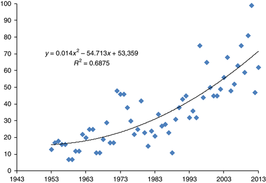
The Federal Emergency Management Agency (FEMA) is the federal government agency which administers disaster assistance and emergency management in the USA. If the President declares a major disaster, FEMA is responsible to coordinate and activate all federal funding programs to start the disaster relief activities. In Figure 2, we calculate and display the trend of the number of declared disasters (y-axis) over time periods (x-axis) in the USA using the data in FEMA’s disaster database (Disaster Declarations, 2013). It clearly shows an upward trend with high value of the coefficient of determination, R2. The trend in Figure 2 as well as the recommendations from Houguín-Veras et al. (2007) motivates the study for an ERSC design presented in this paper.

Emergency relief means “monies or services made available to individuals and communities that have experienced losses due to disasters such as floods, hurricanes, earthquakes, drought, tornadoes, and riots” (Academic Dictionaries and Encyclopedias, 2013). Indeed, after an emergency, it is urgent for an emergency management organization to distribute relief items to the affected areas efficiently and effectively for rapid recovery through emergency response facilities (ERFs). An ERF is a temporary or permanent place where emergency relief items are stored, classified, sorted, and distributed. In other words, logistics planning in the emergency management context involves the rapid and efficient distribution of emergency relief items from ERFs to the affected areas via a transportation network. The ERFs considered in this paper consist of:

1. distribution warehouses (DWHs), where emergency relief commodities are stored;

2. intermediate response facilities names as Break of Bulk (BOB) point or Commodity Distribution Point (CDP), where people can more effectively gain access to relief items; and

3. neighborhood locations in need of relief items and supplies.

The ERSC design is inherently strategic and long-term planning in nature since its ERF location decision requires significant financial resource and the preparation time, and its results cannot be overturned in short-term. The primary objective of this strategic-level decision is to strengthen the disaster preparedness by determining the locations of DWHs and BOBs, distribution channels of emergency supplies throughout the ERSC, and assignment of neighborhood locations to BOBs and BOBs to DWHs. These are important steps in designing an ERSC, and they significantly affect the performance of the resulting ERSC. Traditionally, the transportation or logistics cost has been considered as a main performance measure guiding these design steps. Many traditional cost minimization-based facility location models implicitly assume that located facilities will always be in service or be available and hardly consider the impact of disasters on the facilities. However, in case of emergencies from disasters, some of these facilities may be damaged or completed destroyed. As a result, they cannot provide the expected services. In other words, the ERFs are susceptible to the risks from emergencies. If facilities are damaged, other facilities instead of the initially assigned facilities may have to satisfy the demands of the affected areas. However, this change or response plan probably will increase the transportation cost and time in supplying relief items to the affected areas. Hence, it will be reasonable to consider the vulnerability or a risk level of an ERSC to minimize the disruption cost during the ERSC design along with the transportation or logistics cost.

Furthermore, it is not always possible to provide relief items to populations in all affected locations. In some cases, there may be some limits in terms of coverage due to any access barrier such as a road condition or an inclement weather condition. Therefore, although an ERSC is designed to cover all affected locations in the strategic level, when an emergency occurs, it is still important to evaluate how many demands will be covered by the ERSC under given operational level conditions. The coverage, or covered demand (CDM) may be represented as a function of the distance from a BOB or a DWH. In this study, we use the concept of the maximum coverage distance (MCD) from each ERF to decide whether a neighborhood can be served or not. Dekle et al. (2005) used this concept as a constraint that each neighborhood should be within a certain distance of the nearest BOBs to be served for immediate service. However, instead of directly using the MCD as a constraint, we calculate the CDM at a given MCD, and use it as a performance of measure to evaluate the performance of an ERSC. From this perspective, a network with a higher CDM can supply relief items to more populations if an emergency occurs. Compared to the logistics cost, both the risk level and CDM have not been studied enough. Furthermore, a systematic exploration of the effects of conflicting performance measure is lacking in the literature.

The objective of this study is to provide a framework to design more balanced ERSCs by simultaneously taking logistics cost, risk level, and CDM into consideration. We integrate these three performance measures to guide the ERSC design process. For this, we present a mixed integer programming formulation of the facility location problem, and use a Goal Programming (GP) approach where aforementioned three performance measures are integrated using the weighted sum in the objective function. Then, we analyze the trade-offs or impact of each of these performance measures on resulting ERSCs to evaluate the feasibility and applicability of the framework presented using case studies.

The rest of this paper is organized as follows. After a review of literature in the next section, a GP optimization model is formulated and presented in the following section. Following this, the next section describes case studies and experimental conditions on those case studies. The penultimate section analyzes and discusses results from those experiments. The last section concludes the paper. It also provides recommendations for future research directions.

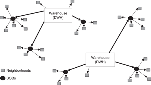
Facility location models have been extensively studied for decades. The network structure in Figure 3 has been frequently used by many researchers. In Figure 3, a DWH can distribute relief items to BOBs (denoted by a thick solid arrow) and neighborhoods (denoted by a solid arrow) and a BOB distributes items to neighborhoods only. Dekle et al. (2005) developed a two-stage modeling approach based on a set-covering model to identify the optimal BOB locations. Their objective is to identify the minimum number of BOBs to satisfy all demands, subject to each county’s residents being within a certain distance of the nearest BOBs. Horner and Downs (2007) studied a similar problem to optimize BOB locations. They formulated a multi-objective integer programming with two objective functions – the first one is to minimize the transportation costs of servicing BOBs from DWHs, and the second one is to minimize the transportation costs between BOBs and neighborhoods in need of relief items.

Snyder and Daskin (2005) presented a facility location model using the p-median approach. They adopted the concept of “failure cost” which is triggered when one or more facilities fail. When an extra facility exists, they reduced the failure cost at the expense of system operating cost. They analyzed the “trade-off” between the operating cost and the expected failure cost of a facility location design. Hassin et al. (2013) investigated the impact of failure of network edges in a facility location problem. The objective function is to maximize the expected post-disaster demand that can be served. A demand location is assumed to be served by a facility if it is located within a certain distance of the facility survived after disaster. They formulated a dynamic programming model, and solved it using a greedy heuristic algorithm.

Shukla et al. (2011) studied the trade-off between efficiency and robustness in an automobile supply chain design. They defined the operational cost-based efficiency and the expected disruption cost-based robustness. To our best knowledge, this is the first paper which attempted to make balance between efficiency and robustness. Their traditional supply chain consists of a manufacturing center, warehouses, and customer zones. They decided the location of warehouses by taking into consideration of both efficiency and robustness under diverse disrupted scenarios. Based on their models and scenarios, their balanced supply chain network in terms of the efficiency and robustness generated less amount of long-term cost. Hong et al. (2012) presented three different distribution strategies using the same logistic network structure as in this study: a BOB is supplied by a specific DWH; by primary and secondary DWHs; and by any DWH. They evaluated these strategies under diverse DWH shutdown scenarios, and reported that overall the third strategy generated the most robust result, the solution with the smallest disruption of the transportation costs. Hong et al. (2013) attempted to design a balanced emergency logistics network using the total logistics cost (TLC) and the expected quantity of disrupted relief items together.

Kanoun et al. (2010) applied GP to select a best location for a new fire and emergency service station for the city of Sfax region in Tunisia, considering several conflicting objectives. The nine sites, none of them could simultaneously optimize all objective, were selected. The developed GP model found for the best compromised site that maximizes the decision maker’s satisfaction and respects the budgetary constraints.

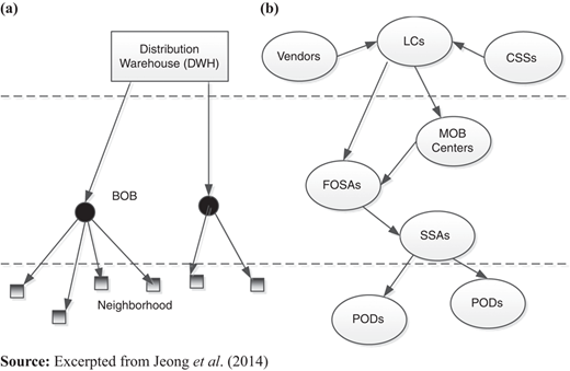
Jeong et al. (2014) compared their ERSC structure to that of FEMA’s in the USA as seen in Figure 4. FEMA has seven major components in its logistics network structure – see Figure 4(b) – while our model has three layered structure as shown in Figure 4(a). As displayed in Figure 4(b), the highest components in FEMA’s model are permanent facilities. They include logistics centers (LCs), Vendors, and Commercial Storage Sites (CSSs). LCs are federal or commercial agency owned facilities that store and distribute relief items to lower level components. The items or goods stored there are supplied from other federal agencies, vendors, or private industry. CSSs are facilities owned by private industry. CSS supports LCs by storing and distributing relief items. The second highest components are temporary facilities which include Mobilization (MOB) centers, Federal Operations Staging Areas (FOSAs), and State Staging Areas (SSA). MOB centers and FOSAs are temporary federal facilities where received items are stored. Both are supplied by higher level LCs. However, FOSAs can also be supplied by MOB centers. SSAs are temporary facilities supplied by FOSAs and located at affected states where items are received and stored for Points of Distribution Sites (PODs). PODs are the lowest temporary facilities located in affected areas at which the relief items are distributed to victims. LCs supply relief items to MOB centers or FOSAs based upon the supports from vendors and CSSs. Note that a DWH in our study is equivalent to a LC or a CSS. A BOB is equivalent to an MOB center or a FOSA and our neighborhoods are equivalent to PODs in the FEMA’s model.

Afshar and Haghani (2012) adopted FEMA’s logistics structure to develop a mathematical model for integrated logistics operations in response to natural disasters. They tried to minimize the total amount of weighted unsatisfied demand where the demand at each location is weighted based on its urgency. Based on this objective function, they decided the optimal locations of three types of temporary facilities in the second highest level in Figure 4(b).

Our study is the extension of the accomplishments done by Shukla et al. (2011), Hong et al. (2012, 2013), and Jeong et al. (2014). Our study overcomes and extends previous works: first, network structure in this research is much more complex. For example, our ERSC considers three layered structures with two dynamic layers – DWHs and BOBs – while Shukla et al. (2011) and Afshar and Haghani (2012) considered only one dynamic layer – warehouses and temporary facilities, respectively; second, we attempt to make balance among three factors rather than two factors as in Shukla et al. (2011), Hong et al. (2013), and Jeong et al. (2014); and finally, based on these, we believe that our approach is more realistic and appropriate to realize the concept of the balanced ERSC than that in the previous studies.

Let M be the set of all neighborhoods and potential DWH locations, indexed by m ∈ M we separate M into two sets: M={N, I}, where I denotes the set of potential DWH locations, i ∈ I (indexed by i=1, 2, …, w) and N represents the set of neighborhoods (indexed by n=1, 2, …, p). In this research, we assume BOBs can be located at any neighborhoods and potential DWH locations, while a DWH can be built at candidate DWH locations only since a DWH requires stronger site conditions – note that a DWH is considered as a permanent facility while a BOB is not as in FEMA’s logistics network structure in Figure 4(b). Based on these assumptions, let j be the set of potential BOB locations indexed by j ∈ {M}, where j=1, 2, … p, p + 1, p + 2, … p + i, … p + w. The notation used in the formulation is as follows:

Notations

a_i   fixed cost for constructing and operating DWH_i

b_j   fixed cost for constructing and operating BOB_j

d_ij   distance between DWH_i and BOB_j

d_im   distance between DWH_i and location m

d_jm   distance between BOB_j and location m

Bmax  maximum under BOBs can be built (set to 5)

(Equation 1) capacity of DWH_i (2,500 K for each DWH in this study)

(Equation 2) capacity of BOB_j (set to 1,500 K for each BOB in this study)

h_m   demand of location (can be either neighborhood or DWH) m

Wmax  maximum number of DWHs can be built (set to 2 in this study)

v_i   minimum number of neighborhoods DWH_i can directly handle (0 in this study)

V_i   maximum number of neighborhoods DWH_i can directly handle (0 in this study)

k_i   minimum number of BOBs a DWH must handle (set to 1 in this study)

K_i   maximum number of BOBs a DWH can handle (set to 10 in this study)

l_j   minimum number of neighborhoods a BOB needs to cover (set to 2)

L_j   maximum number of neighborhoods a BOB cover (set to 7)

Decision variables

B_j   1 if neighborhood j is selected as a BOB, 0 otherwise (decision variable)

W_i   1 if a candidate warehouse i is selected, 0 otherwise

x_ij   1 if BOB_j is covered by DWH_i, 0 otherwise

(Equation 3)   1 if location m is covered by DWH_i, 0 otherwise

y_jm   1 if location m is covered by BOB_j, 0 otherwise

z_ijm   1 if location m is covered by DWH_i through BOB_j, 0 otherwise

The first goal is to minimize the total logistics (transportation) costs. Given this problem setting, the TLC is given by:

(Equation 4) 

where:

(Equation 5) 

The first, second, and third bracketed terms in objective function (1) represent the transportation cost from DWHs to BOBs, from BOBs to neighborhoods, and from DWHs to neighborhoods directly without through BOBs, respectively. Equation (2) defines the decision variable z _ijm, which will be linearized in constraints (20) later.

When a disaster occurs, some of ERFs may be damaged. Consequently the relief items from the damaged facilities may be unavailable (or may not be distributed). Hence, it will be important to locate ERFs at minimally risked areas, so that the quantity of relief items lost due to facility shutdown or damage is minimized. We define the expected quantity of relief items lost as the Expected Number of Disrupted Item (EDI), and use this to measure the level of risk in an ERSC. If we assume that when a facility is shut down due to a disaster, all relief items stored in that facility are lost and if a risk probability (i.e. the probability that a facility is shut down) for each facility is known, then EDI can be expressed as:

(Equation 6) 

where p(i) is the probability that the DWH _i is shut down (or risk probability), q(j) is the probability that the BOB _j is shut down (or risk probability).

If a DWH _i is closed with the probability p(i), all quantity of relief items stored at that location, ∑_j∈M∑_m∈M (Equation 7), is lost. Note that (Equation 8) represents the quantity directly delivered to neighborhoods from DWHs while ∑_j∈M∑_m∈M(z _ijm h _m + h _i W _i) represents the quantity delivered through BOBs. Hence, the second bracketed term represents the expected total quantity of relief items lost at DWHs. If DWH _i is not closed with probability 1 − p(i), then BOB _j is supplied with its full quantity ∑_m∈M(y _jm h _m) and this whole quantity will be exposed to a risk with probability q(j) at BOB _j.

Then, the expected quantity of relief items lost at BOB _j is represented as (1−p(i))∑_m∈M(y _jm h _m)q(j), which is rearranged into the first bracketed term in Equation (3).

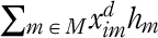
In case of an emergency, a disrupted event may prevent disaster management organizations from distributing relief items to all populations or victims in affected areas. That is, it is not always possible to satisfy all relief demand. Therefore, we also need to evaluate how many demands an ERSC can really satisfy if an emergency occurs. If a neighborhood is within the maximum distance from the nearest ERF, then that neighborhood can be served by the ERF. Otherwise, it cannot be served. Letting D c denote MCD in case of an emergency, then CDM can be expressed as:

(Equation 9) 

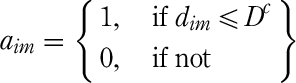
where indicator parameters, a _jm, and a _im are:

(Equation 10) 

and:

(Equation 11) 

The first, second, and third terms in Equation (4) represent the covered demand at neighborhoods by BOBs, at BOBs by DHWs, and at neighborhood by DWHs, respectively. Equation (5) checks whether a neighborhood is within the maximum distance D c from BOB _j and DWH _i, respectively.

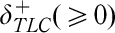
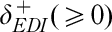
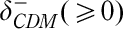
Let TLC _min and EDI _min be the minimum of TLC and EDI obtained from all alternative ERSCs, respectively, and CDM _max be the maximum of CDM obtained from those alternatives. Then the deviation variables, (Equation 12) and (Equation 13) can be defined as surplus, by which each value of TLC and EDI deviates from TLC _min and EDI _min respectively. The deviation variable (Equation 14) is defined as deficiency by which CDM deviates from CDM _max. Then the weighted sum of the percentage deviations is defined as:

(Equation 15) 

where α _g, g=1, 2, and 3, is a weight factor ranging from 0 and 1 and ∑_gα_g=1.

Setting up (6) as an objective function, we formulate a GP model as follows:

(Equation 16) 

subject to:

(Equation 17) 

(Equation 18) 

(Equation 19) 

(Equation 20) 

(Equation 21) 

(Equation 22) 

(Equation 23) 

(Equation 24) 

(Equation 25) 

(Equation 26) 

(Equation 27) 

(Equation 28) 

(Equation 29) 

(Equation 30) 

(Equation 31) 

(Equation 32) 

The objective function in Equation (7) is the weighted sum of the percentage deviations of three performance measures from their target values. Constraints (8) define the upper bound of the number of DWHs that can be built. Here at most W max is allowed. Constraints (9) ensure that the potential DWH location will not be selected simultaneously as both DWH and BOB. Constraints (10) ensure that if a potential DWH location i is not selected (i.e. W _i=0) its demand must be satisfied by a BOB or a DWH. Constraints (11) make certain that each neighborhood (n ∈ N) is assigned to either a BOB or a DWH. Constraints (12) limit the minimum and maximum number of BOBs to be served by each DWH. Constraints (13) ensure that DWHs only supply the selected BOBs. Constraints (14) limit the total number of selected BOBs to be less than or equal to a user-specified number, B max. Constraints (15) ensure that neighborhoods or unselected DWH locations can only be assigned to the selected candidate BOBs. Constraints (16) ensure that the selected candidate BOB _j must cover a minimum number of l _j neighborhoods and can only cover a maximum of L _j neighborhoods. Constraints (17) and (18) show the shipping capacity of BOBs and DWHs, the amounts, respectively. Constraints (19) ensure that a DWH can directly supply at least v _i and at most V _i neighborhoods/unselected DWH locations. Constraints (20) show the upper and lower limit of a linearized variable, z _ijm. Constraints (21), (22), and (23) define the deviation variables representing the amount by which each goal deviates from its target value, TLC _min, EDI _min, and CDM _max.

In this section, we attempt to demonstrate the applicability of the mathematical model given by Equations (7)-(23) using the GP approach. We perform two case studies using the major disaster declaration records in South Carolina (SC). The problem instance described in Jeong et al. (2014) is used in this paper. The Excel Risk Solver platform is used for all experiments.

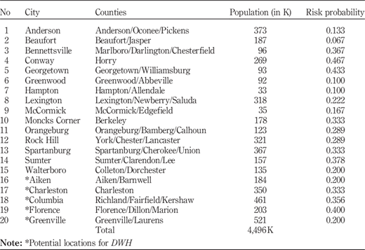
There are 46 counties in SC and they are clustered based on proximity and populations into 20 counties. Then, we choose one city from each clustered county using a centroid approach and assume that all population within the clustered county exists at that city. According to FEMA’s annual disaster declaration record (Disaster Declarations, 2013), SC has experienced 15 major natural disaster declarations from 1964 to 2013. The database also provides a list of counties where a major disaster has been declared. Jeong et al. (2014) assumed that when a major disaster is declared, the ERF in that county is damaged and shut down. Based on this assumption and the historical record, the risk probability for each clustered county is calculated. For example, in Table I, the city “Anderson” represents the clustered county with three counties: Anderson, Oconee, and Pickens. According to SC FEMA’s disaster declaration record, two major disasters were declared in the clustered county from 1964 to 2013. Therefore, the risk probability 0.133 (2/15) is calculated. Each selected city, associated clustered counties, populations, and risk probability are displayed in Table I. The table also shows the potential five locations for DWHs, Aiken, Charleston, Columbia, Florence, and Greenville, in the last five rows starting from the 16th row. They are selected based upon population, the proportion of area that each location could potentially cover, and the proximity to interstate highways in SC. Although not displayed, we have calculated actual distances between cities representing a clustered county and those distances are considered to be the distances between clustered counties.

To demonstrate how the proposed GP model works, the following simplification and parameter setting steps are completed:

1. Objective function given by Equation (1) is simplified by excluding the fixed cost terms for BOBs and for DWHs.

2. The numbers of BOBs and DWHs to be built are pre-specified as follows. The maximum numbers of BOBs and DWHs that can be built, B max and W max, are set to 5 and 2, respectively. The minimum and maximum number of BOBs that a DWH must handle, k _i and K _i, are set to 1 and 10, respectively, among many different values. The selected value for B max and W max seems to be best for demonstrating the trade-offs and correlations among three key objectives for our case study. The minimum and maximum number of BOBs that a DWH must handle, k _i and K _i, are set to 1 and 4, respectively, since at most two DWHs should cover at most five BOBs.

3. Each BOB must handle at least 2 neighborhoods (l _j=2) and at most 7 (L _j=7). It implies that a BOB will cover the neighborhood, where it is located, plus at least one other neighborhood. Each BOB must at most 7 (L _j=7), to prevent one BOB from covering more than 7. For simplicity for our analysis, we set V _i=0, ∀i.

4. The capacity of a BOB and a DWH is set to 1,500 and 2,500 K in terms of the quantity of relief items. These capacities are set after considering that the total demand for two DWHs to cover is 4,496 K and for at most five BOBs to cover is 4,496 K minus the demand for the two DWH locations.

5. We set MCD in the case of emergency, D c in Equation (5), to 35 miles for Case Study I and 62 miles for Case Study II. That is, if a neighborhood location is within this distance from a BOB or a DWH, that location can be served by that facility.

6. In calculating CDM, we assume that a BOB is still supplied by the assigned DWH although the BOB is beyond MCD from the DWH in case of an emergency. In other words, MCD is applied to neighborhoods only.

Before solving the GP under diverse conditions, all upper and lower bound values should be calculated first. TLC _min is obtained by solving the minimization problem with Equation (1) as an objective function and constraints (8) through (20). Similarly, EDI _min in Equation (3) is obtained from the same minimization problem but with the different objective function. The first case study uses the maximum coverage distance, D c, set to 35 miles while the second case study uses D c set to 62 miles. The CDM _max in Equation (4) is obtained from the maximization problem. The results are summarized in Table II. As D c increases from 35 miles to 62 miles, CDM _max increases from 3,545 K (79 percent of the total populations) to 4,496 K (100 percent of the total populations).

Using the upper and lower bound values in Table II, we solve the GP model for various values of α _g. Each α changes between zero and one with 0.1 as an increment. Thus, there are 66 configurations arising out of the combinations of the setting of α under the condition α ₁ + α ₂ + α ₃=1 for each case study. From here, we omit the symbol “K”, 1,000, in describing numbers.

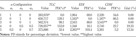
With D c set to 35 miles, Table III displays the results of five extreme configurations out of 66 configurations where each configuration is decided by different combinations of (α ₁, α ₂, α ₃). These are extreme configurations in the sense that the resulting ERSCs are extremely unbalanced among performance measures. The first three configurations generate TLC _min, EDI _min, and CDM _max, respectively. Therefore, all of these three configurations generate zero percent deviation (PD) where each α _g is set to 1, resulting in zero in the objective value (G). For example, the first configuration, (1, 0, 0), considers the TLC minimization only with α ₁ set to 1. Therefore, it exactly produces TLC _min Hence, its deviation from TLC _min is zero. Since none of EDI and CDM is considered, resulting EDI and CDM values are much higher and lower than EDI _min and CDM _max, respectively. The same reasoning is applied to the second and third configuration in terms of TLC and CDM, and TLC and EDI, respectively. The fourth configuration generates the result with the highest TLC while the last row represents the configuration with the highest EDI. Note that the second configuration generates the lowest EDI (1,162) but the lowest CDM (1,187) at the same time, indicating that without appropriate balance, the resulting ERSC shows the best performance in terms of risk but the poorest coverage if an emergency occurs.

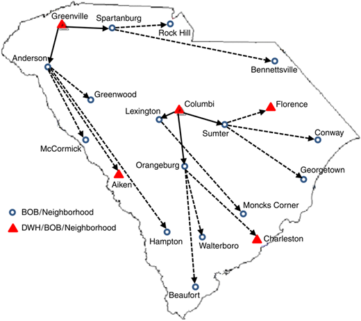
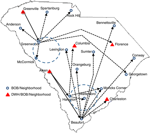
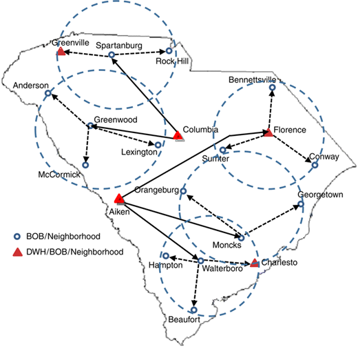
Figures 5, 6, and 7 show the ERSCs corresponding to the first three configurations in Table III, respectively. A solid arrow line represents distribution from a DWH to a BOB while a dotted arrow line represents distribution from a BOB to a neighborhood. Figure 5 displays the ERSC corresponding to (1, 0, 0) configuration, generating 283,976 as TLC _min at the cost of EDI and CDM and the corresponding EDI is 1,964 items consisting of 1,285 items from DWHs and 679 items from BOBs. DWHs at Columbia and Greenville supply 2,474 and 2,022 items, respectively – total 4,496 items, satisfying all demands – through their BOBs. Using the risk probability of Columbia (0.356), and Greenville (0.2) in Table I, the EDI at DWHs is calculated as 1,285=2,474(0.356) + 2,022(0.2), while remaining 679 items are calculated from EDIs at five BOBs in a similar way. If an emergency occurs in this network, none of the neighborhoods is supplied from BOBs and DWHs since it is not located within 35 miles from a BOB and a DHW. Therefore, its resulting CDM is just the sum of all populations from DWHs and BOBs, 2,320 without any population from a neighborhood according to the last simplification and parameter setting step described previously. Finally, the ERSC in Figure 5 shows an example of an unbalanced ERSC sacrificing other two performance measures for generating the minimum TLC. Figure 6 represents the safest ERSC from an EDI perspective at (0, 1, 0), generating EDI _min at the cost of TLC and CDM. We can see that two safest DWHs, Greenville, and Aiken with their risk probability 0.2 each are selected to minimize EDI to 1,162 items. However, this makes the distribution routing very complex, exacerbating TLC to 650,717. Further, in case of an emergency, this configuration will cover only the lowest amount of CDM, 1,187. The total populations of all selected BOBs and DWHs are 1,017 according to Table I. The dotted circle represents the distribution to the neighborhoods located within maximal coverage distance (MCD) from a DWH or a BOB. In this case, McCormick supplied by Greenwood and Walterboro supplied by Hampton are those. Adding their populations to 1,017 generates 1,187 as CDM.

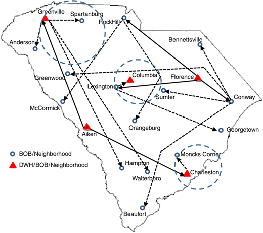
The ERSC corresponding to the third configuration, (0, 0, 1), in Table III is displayed in Figure 7. This will cover the highest demand, 3,545, for the case of an emergency, at the cost of TLC and EDI. In other words, if an emergency occurs, only three distribution channels will be still available. Note that there are 20 locations in the map, and 11 locations out of the top 12 most populated locations are selected as a BOB, a DWH, and a neighborhood to maximize CDM. For example, Greenville (the city with the largest population) serves as a BOB supplied from Aiken, and Columbia (the city with the second largest population) serves as a neighbor supplied from Lexington. The sum of total populations from those 11 locations is 3,545.

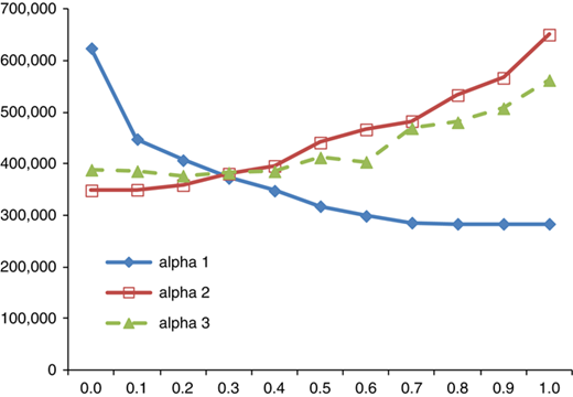
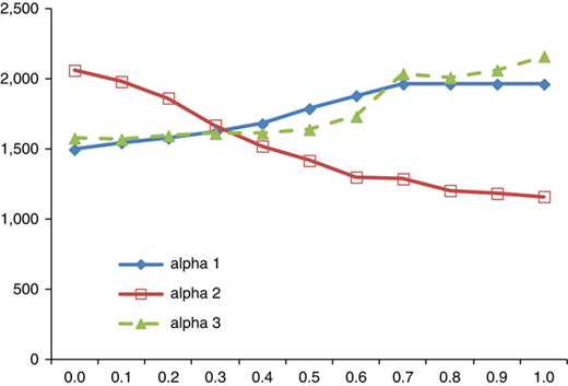
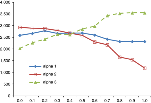
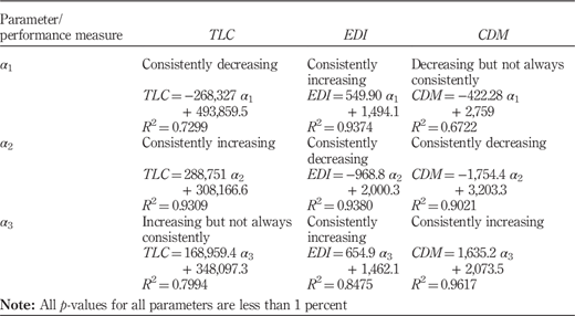
To see the effect of variation of α _g’s on TLC, EDI, and CDM, Figures 8, 9 and 10 display the average values of those three performance measures (y-axis) against α _g’s (x-axis). As α ₁ increases (or TLC is more addressed), GP tends to generate a more cost efficient network, consistently reducing TLC (Figure 8). However, at the same time, this cost-oriented approach increases the risk of the ERSC, consistently increasing EDI as seen in Figure 9. We can also observe that as α ₁ increases CDM decreases although this trend is not always consistent (Figure 10). With increment of α ₂ (or EDI is more addressed), GP tends to reduce the risk of ERSCs, consistently reducing EDI (Figure 9). At the same time, this increases TLC (Figure 8). Figure 10 indicates that as EDI gets more addressed (α ₂ increases), its CDM decreases. That is because that as EDI decreases, the routing for distribution may be more complex, and this may increase the chance to assign a BOB to more remotely located neighbors to reduce risk. Therefore, this will deteriorate CDM in case of an emergency. As α ₃ increases (CDM gets more addressed), CDM and EDI consistently increase as seen in Figures 10 and 9, respectively. However, TLC roughly increases but not always (Figure 8).

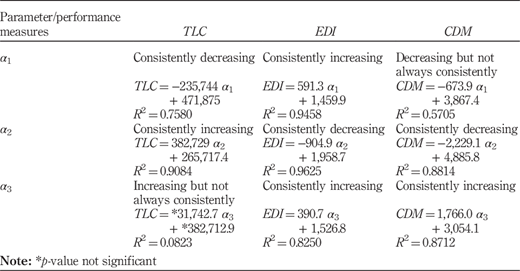
Table IV summarizes the trend of TLC, EDI, and CDM over α _g’s using linear regression and relevant R2 value with verbal descriptions of their effect. It clearly shows: first, TLC and EDI have a clear trade-off relationship with each other in terms of α ₁ and α ₂. For example, TLC and EDI move in an opposite direction when α ₁ or α ₂ changes. However, they move together on α₃; second, EDI and CDM move together in terms of α ₂ and α ₃. For example, both decrease as over α ₂ increases and both increase as over α ₃ increases. However, they have a trade-off relationship over α₁; and finally, TLC and CDM have a trade-off relationship in terms of α ₂ while both move together over α ₁ and α ₃. Based on the slopes of the regression lines, α ₁ and α ₂ have higher impact on TLC than α _3. On EDI, and CDM, α ₂ and α ₃ have higher impact.

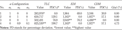
The second case study uses the same data except D c set to 62 miles. Table V displays four extreme results out of 66 configurations. The first three configurations generate TLC _min, EDI _min, and CDM _max, respectively. Note that the second configuration (0, 1, 0) generates the lowest EDI (1,163) and the lowest CDM (1,927) together, and the third configuration (0, 0, 1) generates the highest EDI (2,049) and CDM (4,496), simultaneously. The second (0, 1, 0) and the fourth configuration (0, 0.9, 0.1) generates the alternative solutions for EDI and CDM but not for TLC.

Figure 11 shows the ERSC generating CDM _max based on the configuration (0, 0, 1). Note that all neighborhoods are within 62 miles from all BOBs. Consequently, CDM turns out to be 4,496 enough to cover all populations, shown as in Table II, at the cost of EDI and TLC. The patterns of TLC, EDI, and CDM on α ₁, α ₂, and α ₃ are very similar to those in Case Study I. However, the magnitude of impact is different because of the difference in CDM. Table VI summarizes the regression lines and R2 values again. While most of the lines show the same patterns, the regression line of TLC on α ₃ has low R2 value and its parameters are not significant. Therefore, when compared to the corresponding cell in Table IV in Case Study I, the effect of α ₃ on TLC is less apparent.

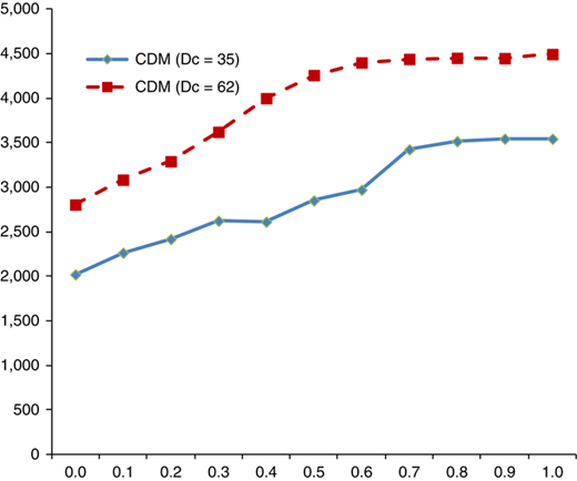
We compare the impact of MCD on CDM for both cases in Figure 12. The CDM (y-axis) for both cases consistently increases and its marginal increment gets smaller when α ₃ (x-axis) increases (CDM gets more weight).

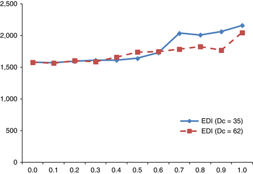
Figure 13 plots the impact of α ₃ (x-axis) on EDI (y-axis) for both case studies. Both cases have a similar pattern. When CDM gets more emphasized, it tends to exacerbate EDI at both cases. The chart also indicates that when MCD is larger, EDI is less sensitive to CDM. This occurs that the case with larger MCD can generate more alternative distribution networks, which contribute to minimizing EDI than does the other case.

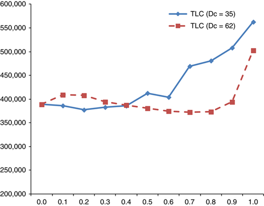
Figure 14 shows the impact of α ₃ (x-axis) on TLC (y-axis) for both case studies. This is the only case where the pattern between two case studies is significantly different. In Case Study I (D c = 35), as CDM gets more weight, there is a clear upward trend in TLC. However, TLC within Case Study II (D c=62) does not show such a clear upward trend as analyzed in the cell labeled referenced by (α ₃, TLC) in Table VI. Again, since the larger MCD generates more alternatives than does the smaller MCD, some of those alternatives generate smaller TLC.

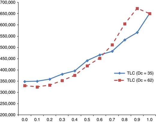
Figure 15 plots the impact of α ₂ (x-axis) on TLC (y-axis) since MCD can affect EDI, and TLC can be affected by EDI again. Both case studies have the same pattern of TLC over α ₂. However, when EDI is less emphasized in the objective function (when α ₂ is smaller than or equal to 0.6), the case with D c=35 miles has higher TLC. When EDI is more emphasized (when α ₂ is larger than or equal to 0.7), the other case has higher TLC.

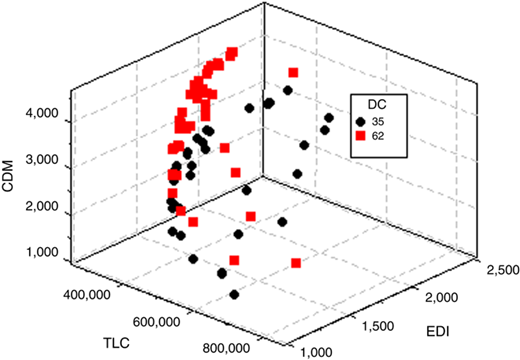
Figure 16 displays results from all configurations in both cases. The graph indicates that many points with Dc=62 have higher CDM and lower TLC. Hence it partly supports the conclusion in Figures 12 and 14. However, other information is not apparent. Table VII summarizes the average values of three performance measures in both case studies. The average values of TLC and EDI in Case Study II are reduced by 2.8 percent and 1.2 percent, respectively, while the average value of CDM increases by 39.1 percent. It clearly supports the conclusions in Figures 12, 13, and 14. In other words, a larger MCD seems to generate favorable results in terms of each performance measures analyzed in this study due to the increased flexibility of ERSC. However, it is sometimes impossible to have a larger MCD in case of a severe emergency.

In this paper, we consider an ERSC design problem, where the TLC, the EDI, and the total amount of CDM in case of an emergency are considered major performance measures. We propose the GP-based-framework for the ERF location and allocation problem, taking those three performance measures into consideration, simultaneously. We analyze their trade-off relationship through realistic case studies.

Two case studies have been provided to demonstrate the proposed model’s capability to deal with uncertainties in designing balanced ERSCs. Each case study has been analyzed thorough the experiments with 66 configurations for various weights: α₁ for TLC, α₂ for EDI, and α₃ for CDM under maximum coverage distance, Dc. From the numerical results through those case studies, we have observed the following phenomena: as the logistics cost factor gets more emphasized (α₁ increases), the TLC generally decreases, however, the resulting ERSC has a higher risk level with increasing EDI as well as less CDM. As the risk factor is more emphasized (α₂ increases), the network gets more stable, generating smaller EDI at the expense of TLC. This risk-averse ERSC tends to make distance between a BOB and neighbors farther, reducing CDM. Once the covered amount of demand factor is more emphasized (α₃ increases), we notice that all three performance measures increase together. The study also reveals that MCD has positive effect on ERSC. It directly increases CDM, and overall tends to reduce TLC and EDI by providing more alternative network layouts. However its impact on EDI is smaller than that on other two performance measures.

The present study has significant theoretical and practical implications in terms of its applicability. The nature of disaster management will require in-depth study of many conflicting performance measures. In our study, we have considered three of those performance measures. They are conflicting and correlated each other. For example, TLC and EDI are conflicting in terms of α₁ and α₂. TLC and CDM are conflicting in terms of α₂. Finally, EDI and CDM are conflicting with respect to α₁. Therefore, it is not possible to incorporate all relevant performance measures into a single objective function without weighting these performance measures in an objective function. However, this approach will require prior determination of those weights and will make balancing of major performances more difficult. Instead, we have conducted detailed trade-off analysis by changing those weights between zero and one. Using this GP-based-weighted objective function and the trade-off analysis, we have identified that all performance measures should be balanced in designing ERSCs. Otherwise, the resulting ERSC will significantly sacrifice other performance measures unintentionally.

This study presents useful overviews and insights to practitioners in the disaster management discipline. The result indicates that decision makers in any emergency management organization can make their decision on ERSC design and response by taking cost, risk, and coverage into consideration together, selecting alternatives based on trade-off relationships among those metrics. In addition, if time and computing resource are allowed, the practitioners can visualize these trade-off relationships through all configurations as seen in Figure 16. In this way, they can choose an appropriate alternative under specific situations. Another important result supported from the trade-off relationship is that an emergency management organization shall need to acquire diverse capabilities to improve its MCD in the operational level to earn favoring TLC and EDI. Practitioners may secure more road repair equipment and manpower or emergency transportation vehicles etc. to increase the MCD.

Other than the three performance measures presented in this study, emergency relief planner may consider additional factors that are crucial for the ERSC design and planning process. The factors that we identified include but not limited to the following: response time, total unsatisfied demand, relief goods variety (meal, water, medicine, etc.), relief goods availability, fifth, victim service levels, multimodal transportation network including road conditions, and contingency plan (identifying backup road(s), BOBs, and DWHs). These aforementioned factors could be incorporated and applied in the decision-making process for emergency management in practice. First, as depicted in Figure 4, our ERSC structure is similar to FEMA’s logistics supply chain. Hence, our proposed model can be adopted and applied for FEMA or other federal or state emergency management agencies. Second, since our model is coded and solved in Excel®, it is user-friendly for practitioners to use. The simple user interface allows users to input their input parameters and obtain results effortless.

As we must face the reality that millions of people and hundreds of areas and regions are exposed to risk from various disasters and catastrophes within next decades, the framework similar to one presented in this paper would be highly desirable. For a future research agenda, both researchers and practitioners may consider other performance metrics not includes in this paper. In fact, one of the contributions of this study is that it presents the GP based-framework. That is, other factors can be integrated into our propose model if operational-level definition is appropriately made. For instance, response time, total unsatisfied demand, victim service levels can be added to the objective function. Relief goods variety, availability, multiple transportation modes may be considered in the model’s constraints. Contingency plans can be obtained through regenerating plans based on the changing demand, facility capacity size, and disrupted distribution routes. However, considering all the factors may complicate the model and make the model intractable. Therefore, researchers and practitioners can qualitatively choose the top priority performance measures and then use the GP model. Alternatively, heuristic methods can be developed to obtain near-optimal solution.

It may be interesting to include other goals, such as minimizing the maximum coverable distance, and to investigate the effect of each goal on the optimal locations and allocation among ERFs. Although our study attempts to integrate both strategic and operational measures together, this type of integration still needs more study. Based on more realistic and operational-level data such as diverse paths and/or the conditions of these paths, the integration of vehicle routing between locations along with ERSC design problem we consider in this paper would improve the applicability of this research.

BOB  break of bulk

CDM  covered demand

CDP  commodity distribution point

DWH  distribution warehouse

EDI  expected number of disrupted relief items

ERF  emergency response facility

ERSC  emergency relief supply chain

FEMA  federal emergency management agency

GP  goal programming

MCD  maximum coverage distance, Dc

PD  percentage deviation

TLC  total logistics cost

Dr Jae-Dong Hong is a Professor in Industrial Engineering Technology at the South Carolina State University. He holds a BS from the Korea University, Seoul, S. Korea, an MS and a PhD from the Penn State University, all in Industrial Engineering. His research interests are in the areas of large-scale optimization using VBA in Excel and modeling of various logistics problems using spreadsheet. He has published more than 50 technical papers in various international journals and proceedings. He is the recipient of many prestigious awards, including the South Carolina Governor’s Distinguished Professor of Year Award. He has been recognized in various Who’s Who and ranked in the top 20 operations management researchers in terms of research productivity and quality in the survey in Journal of Operations Management.

Dr Ki-Young Jeong is the Program Chair of Engineering Management at the University of Houston-Clear Lake (UHCL). Dr Jeong holds his MS and PhD in Industrial Engineering from the Texas A &M University and Professional MBA from the University of Massachusetts at Amherst. His current research interests include operations management, decision support system, modeling and simulation, supply chain management, and project management. He is an author of more than 30 papers in refereed journals and conference proceedings. He has published articles in International Journal of Operations and Production Management, Expert Systems with Application, Business Process Management Journal, Journal of Industrial Engineering and Management, International Journal of Operations Management Education and International Journal of Logistics. He serves as an editorial board member for Production, Logistics, Quality, and Operational Research in Journal of Industrial & Engineering Management and as international editorial review board member in International Journal of Applied Industrial Engineering. Dr Ki-Young Jeong is the corresponding author and can be contacted at: jeongk@uhcl.edu

Dr Keli Feng is an Associate Professor of Business Administration at the South Carolina State University. He received his PhD degree in Operations Management from the University of Cincinnati in 2005. His research interests are in area of Supply Chain/Logistics Management, Production & Inventory Management and Simulation of Logistics Systems.

This research is supported by the grants from the 1890 Institution Teaching, Research and Extension Capacity Building Grants Program of the National Institute of Food Agriculture (NIFA), US Department of Agriculture (USDA).