


This study adopts a data-driven analytical framework to examine homestay pricing, combining machine learning models with model-agnostic explanation tools. Compared with traditional hedonic pricing approaches, it provides complementary and more transparent evidence on how facilities and services contribute to price formation, and offers preliminary insights into their implications for resource allocation.
Using data from 3,054 homestays in the Qiandao Lake area, this study constructs a three-tier feature system covering property attributes, facility configuration and service management. An XAI framework that integrates XGBoost with SHAP-based interpretability is then employed to quantify the dynamic contributions of these features to observed prices.
Significant nonlinear effects govern pricing. For example, a bimodal distribution emerges with respect to distance from attractions. SHAP-weighted facility/service indices outperform individual attributes in explaining price variation. High-value features drive price premiums, whereas excessive facility investment exhibits threshold effects and diminishing returns. Additionally, we conduct out-of-distribution robustness checks by extrapolating to a peak-season window with mean re-leveling and by re-estimating the core relationships via a generalized additive model. Both tests corroborate the transferability of the “Facility Index” and “Service Index” and the stability of key pricing mechanisms across seasons.
The facility and service indices translate complex model outputs into actionable levers. Hosts can prioritize high-impact amenity bundles, calibrate upgrade intensity to avoid over-investment and fine-tune seasonal price ladders for different property types. Destination managers can use the indices to benchmark homestay quality, anticipate price pressures in sensitive zones and design incentive schemes that align infrastructure provision, regulation and support with data-driven evidence.
This research pioneers the integration of explainable machine learning techniques with multidimensional indices, providing actionable strategies for resource allocation and dynamic pricing. The methodology offers novel theoretical insights for industry policy-making and future pricing research.
1. Introduction
While the homestay market is expanding rapidly, pricing practices often lag behind product upgrades, as many operators rely on historical heuristics and struggle to translate high-cost amenities into sustained price premiums. This misalignment between investment and consumer-perceived value is compounded by conventional models' limited ability to capture nonlinearities and complex feature interactions. To address these challenges, we develop a data-driven and XAI-enabled framework that integrates heterogeneous listing attributes and quantifies their marginal contributions to price formation, providing interpretable evidence for constructing facilities and services indexes.
Traditional pricing models fall short of capturing the complexity of homestay markets. Rosen's hedonic pricing model (Rosen, 1974) pioneered the decomposition of attribute value, but its linear framework cannot accommodate the nonlinear synergies among facilities and services or the nonstationary dynamics of homestay pricing. Machine-learning approaches such as XGBoost and random forest improve predictive accuracy by modeling nonlinear relationships, yet their limited intrinsic interpretability obscures how individual features contribute to price formation (Rico-Juan and Taltavull de La Paz, 2021). Sainaghi et al. (2021) describe this tension as a “predictability–interpretability paradox,” which hampers the translation of large data volumes into actionable pricing insights and may ultimately lead to misdirected investment and diminishing returns. Moreover, algorithmic pricing built on opaque decision rules can raise fairness concerns, weaken corporate social responsibility (CSR) and trigger consumer backlash or online firestorms when perceived as ethically questionable (van der Rest et al., 2022).
This widening gap between theory and practice calls for methodological innovation. Building on Sainaghi et al.(2021), who emphasize the foundational role of data-driven paradigms in homestay pricing, we develop an integrated framework that couples explainable machine learning with multidimensional index systems to move beyond linear modeling. Using multi-source data from Qiandao Lake, we employ SHAP-based diagnostics to identify redundancy in high-cardinality categorical features and to refine the construction of facility and service indices. In addition, we stress-test generalization and inference through cross-season extrapolation and a generalized additive model (GAM), using the former to assess predictive robustness and the latter to provide statistical significance tests and confidence intervals. Taken together, this dual lens of prediction and statistical inference strengthens the credibility and policy relevance of the findings and provides a structured path from problem diagnosis to technical solutions and strategic insights.
2. Literature review
Research on homestay pricing has attracted widespread attention as an important subfield of tourism economics with significant practical implications. Homestays are a unique product combining residential and tourism services; their price heterogeneity arises from complex interactions among unobservable factors, which makes the pricing mechanism a challenging area of study. This section reviews relevant literature from three dimensions – theoretical foundations, methodological evolution and model innovation – to clarify the current research position and identify gaps for innovation.
2.1 Theoretical foundations: from housing price to an extended homestay pricing paradigm
Homestay pricing originates in the housing-price tradition. Lancaster's utility-bundle theory (1966) provides the conceptual basis for hedonic pricing, later formalized by Rosen (1974), which treats observed prices as the sum of implicit attribute values. As the field has evolved, pricing strategies diversified (e.g. bundled and dual pricing), yet hedonic specifications remain widely used by tourists (Hassan and Saleh, 2023). In parallel, models have progressively incorporated richer sources of heterogeneity – most notably spatial and spatiotemporal structure. For example, Bowen et al. (2001) introduced spatial variables into a Cuyahoga County housing-price model and revealed spatial autocorrelation; Holly et al. (2011) analyzed the dynamic evolution of London's housing market using spatiotemporal models; and, in China, Zhu and Zhang (2021) adapted Holly's framework to a multi-regional setting suited to the local context.
However, homestay pricing requires particular attention to the distinct characteristics of tourism accommodations. Early studies, such as Portolan (2013), quantified the price impact of features like location, parking availability and sea view. Chattopadhyay and Mitra (2020) analyzed 143 amenities as binary variables, but the lack of data integration diluted the importance of individual features. Rigall-I-Torrent and Fluvià (2011), in studying hotel pricing, found that traditional linear models fail to capture nonlinear interaction effects between amenities – an issue equally relevant to homestays. Latinopoulos (2018) showed in a hotel sea-view pricing study that the premium of a single attribute (a sea view) may be offset by deficiencies in other amenities (insufficient parking), underscoring the limitations of the simple facility-counting approach proposed by Monty and Skidmore (2003).
Despite recognition of facilities/services, two limitations persist: the tendency to impose equal weights on heterogeneous amenities and the difficulty of capturing nonlinear interactions. Relatedly, Bi and Fu (2022) argued that core housing characteristics often dominate price formation, a useful benchmark for disentangling facility – service synergies.
2.2 Methodological evolution: from classical statistics to spatial econometrics
Early Airbnb pricing studies primarily relied on classical statistical models. For example, Lawani et al. (2019) explored the impact of online ratings on pricing; Gunter and Önder (2018) used cluster-robust OLS to find the marginal effects of listing capacity and host experience on price; Lee and Kim(2023) employed a spatiotemporal panel model to investigate how homestay development influences rent and gentrification. However, these studies faced limitations in integrating diverse features and often omitted rich geographic attributes.
The introduction of spatial econometric methods provided a new path to address these limitations. Chica-Olmo et al. (2020) developed a spatial hedonic model for tourist apartments in Málaga, and Hu et al. (2020) combined hedonic pricing with GIS interpolation to study price clustering in Enshi. Gao et al. (2022) used geographically weighted regression (GWR) to reveal spatial differentiation in hotel prices, while Wang and Rasouli (2022) integrated GWR with DeepLabv3-based image segmentation to quantify landscape effects. Jiang et al.(2024) applied multiscale GWR (MGWR) to examine built-environment influences on Airbnb distribution, and Chen and Xie (2017), using a Spatial Durbin Model, identified an 8.3% spillover effect for properties within 1 km of major attractions. Yet these approaches still struggle with high-dimensional categorical variables, and they may overemphasize spatial factors while underweighting intrinsic property attributes in pricing.
2.3 Model innovation: integration of machine learning and explainable AI
Machine learning (ML) advances have expanded the modeling toolkit for housing and homestay prices (Zhang, 2023). Soltani et al. (2022) addressed spatiotemporal nonstationarity by adding lag indicators to ML models on a 32-year Adelaide dataset, and Jiang et al. (2023) – using active Chinese homestay listings – found that in highly accessible areas, the marginal impact of location on short-term rental prices diminishes.
In hotel price studies, ML likewise demonstrates clear advantages. AI models such as ANFIS and deep belief networks outperform traditional statistical approaches in price prediction (Al Shehhi and Karathanasopoulos, 2020). Binesh et al. (2023) use an LSTM model that incorporates game-theoretic and risk factors to forecast hotel ADR for the COVID-19 period, and Ghosh et al. (2023) propose an ensemble framework for predicting Airbnb rental prices that does not rely on amenity-driven features but achieves higher accuracy through feature selection, ensemble learning, particle swarm optimization and explainable AI (XAI).
Beyond pricing, ML and artificial intelligence (AI) also enhance operational efficiency and demand forecasting in the hospitality sector. For instance, Zheng et al. (2024) integrated multi-scale spatiotemporal features to predict hotel demand, while He et al. (2021) developed a hybrid SARIMA-CNN-LSTM model for forecasting tourist arrivals in Macao. Sánchez-Medina and C-Sánchez (2020) advanced cancellation prediction, and Contessi et al. (2024) merged principal component analysis (PCA) with pickup methods for interpretable occupancy forecasts. Collectively, these approaches excel at capturing nonlinearity, high dimensionality and real-time signals, delivering high-frequency, actionable inputs for revenue management.
Despite these advances, accommodation pricing confronts a persistent interpretability challenge: strong in-sample performance seldom translates to causal insights or practical pricing rules. The opacity of many ML models further hampers causal inference, as noted by Zhao and Hastie (2021). Explainable AI (XAI) techniques, particularly SHAP values (Lundberg and Lee, 2017), address this by quantifying feature-level marginal contributions. However, applications in housing and homestay pricing remain limited, often confined to visualization or basic decomposition. Few studies aggregate SHAP attributions across multifaceted facility and service dimensions into composite indices for decision-making, or derive operational thresholds from such aggregations. Moreover, case-specific validations are scarce, underscoring the need to operationalize and rigorously test SHAP-derived insights in real-world settings. Our study bridges this gap by constructing SHAP-weighted indices and evaluating their pricing implications in a homestay context.
Building on the foregoing, three gaps remain salient. First, despite SHAP's global uptake, rigorous SHAP-based analyses of homestay pricing grounded in the Chinese market are scarce; studies that leverage localized datasets – and, in particular, convert SHAP outputs into decision-oriented artifacts – are largely absent. Second, multidimensional categorical attributes are often collapsed into binaries or coarse groupings, obscuring heterogeneous feature weights. Third, the literature tends to privilege linear marginal effects while underexamining interactions, thresholds, complementarities and synergies among facilities, services and property attributes.
2.4 Research positioning and innovation
Building on these gaps, we develop an integrated pricing framework for China's homestay market that aggregates property, facility and service attributes into decision-oriented Facility and Service Indices (FI/SI) using SHAP. The framework relies on a nonlinear learning setup that accommodates heterogeneity and interactions among attributes, and it shifts the focus from model-level explanation to actionable aggregation. In doing so, it demonstrates empirical utility in a localized homestay context.
Our SHAP-based index construction assigns data-driven, prediction-relevant weights that remain valid under nonlinearity and interactions, while still preserving attribute-level semantics within the composite indices. This design also enables the derivation of operational thresholds for pricing and resource allocation. Unlike prevailing practices that either impose additivity or prioritize dimensionality reduction at the expense of interpretability – and unlike prior SHAP applications that stop at visualization or basic decomposition without multi-attribute aggregation – our approach directly links explanatory contributions to pricing decisions through calibrated composite indices. Overall, this study advances explainable machine learning in tourism accommodation by converting model explanations into decision-oriented measures within a localized Chinese homestay setting, thereby addressing the contextual and methodological gaps identified in the literature.
3. Methodology
3.1 Case area overview
Qiandao Lake (Chun'an County, Hangzhou, Zhejiang) is a major destination in the Yangtze River Delta with distinctive landscape resources and a fast-growing homestay sector (Lu and Bao, 2010; Xiang et al., 2019; Yang et al., 2022). Originating from the Xin'an River reservoir project, the destination has developed a diversified accommodation market, shifting from relatively homogeneous farmhouse-style lodgings to more differentiated themed products, such as eco-cabins and lake-view rooms (Wang et al., 2016; Yang et al., 2018).
3.2 Data collection and feature system construction
We assembled a room-level dataset for the Qiandao Lake market covering 500+ homestays, yielding 3,085 records; after screening invalid entries, 3,054 valid listings remained. Data were scraped on January 4, 2025, from publicly accessible pages using the query “Qiandao Lake” and the accommodation-type filter “Homestays.” Given the lag in open-source repositories following Airbnb's exit from China, this live snapshot provides timely coverage of current market conditions around Qiandao Lake. To study pricing, features are organized into a three-tier system – Property Attributes, Facilities and Services (Table 1). Facility/service fields follow the platform's ordinal coding (0 = none, 1 = free, 2 = partly charged, 3 = fully charged). Unreported items are coded as 0 to maintain consistency.
Feature system table
| Feature category | Feature variables | |
|---|---|---|
| Property Attributes (29 features) | Environmental.Rating, Time.Since.Opening, Time.Since.Renovation, Distance.to.Tourist.Attraction.Center, Facility.Rating, Total.Number.of.Reviews, Cleanliness.Rating, Service.Rating, Recommendation.Percentage, Number.of.Rooms, Distance.to.Train.Station, Number.of.Tourist.Attractions.within.3.km, Number.of.Restaurants.within.3.km, Number.of.Shops.within.3.km, Area, Maximum.Capacity, Floor, Platform Partnership Status, Platform.Certification.Level, Window Type, Room Availability Status, Number.of.Photos, Park View, Garden View, City View, Lake.View, Mountain View, Landmark View, Courtyard View | Physical space characteristics (e.g. Maximum Capacity, Area, Number of Rooms, Floor), location characteristics (e.g. Number of Restaurants within 3 km, Number of Shops within 3 km, Number of Tourist Attractions within 3 km, Distance to Tourist Attraction Center), operational characteristics (e.g. Time Since Opening, Platform Certification Level), and market feedback indicators (e.g. Total Number of Reviews, Facility Rating, Environmental Rating, Cleanliness Rating, Service Rating (these ratings refer to the scores given in user reviews)). These features capture inherent attributes and locational endowments of homestays and are relatively stable in the long term |
| Service Management (19 features) | Smoking Policy, 24 Hour Front Desk, Check-in Procedure, Breakfast, Pet Policy, Check-Out Time, Instant Confirmation, Cancellation Policy, Check-in Eligibility Restrictions, Luggage Storage, Laundry Service, Pet-Friendly, Shuttle Service, Car Rental Service, Butler Service, Minibar and Soft Drinks, Bar and Café, Room Service, Welcome Gift | Service offerings and policies including standardized services (24 Hour Front Desk, Check-in Procedure, etc.), policy restrictions (Pet Policy, Smoking Policy, etc.), and value-added services (Shuttle Service, Butler Service, etc.). These service attributes reflect differences in operational management and customer service, playing an important role in guest satisfaction and repeat bookings |
| Facility Configuration (31 features) | Children's Facilities, Swimming Pool, Mahjong Parlor, Tea Room, Restaurant, Conference Hall, KTV, Ecotourism, Parking Lot, Game Facilities, Dive Sites/Fishing Spots/Beach, Hot Springs, Sauna and Massage, Razor, Iron, Home Theater, Smart Toilet, Bathtub, Smart Door Lock, Heating, BBQ Equipment, Duck Down Comforter, Kitchenware, Accessibility, Spare Bedding, Clothes Dryer, Refrigerator, Projector, Planting and Picking, Garden/Terrace/Courtyard, Coffee Maker | Amenities covering basic facilities (Parking Lot, Bathtub, etc.), recreational facilities (Swimming Pool, Mahjong Parlor, KTV, etc.), unique experiential facilities (Dive Sites/Fishing Spots/Beach, Planting and Picking, etc.), and business facilities (Conference Hall, Tea Room, etc.). These hardware features directly influence guest experience and are more variable than the fixed property attributes |
This study does not involve direct interaction with guests or hosts. All data were obtained from publicly accessible homestay platforms and contain only anonymized listing- and transaction-level information. Homestay names, host identities, contact details and other personally identifiable information were neither collected nor stored. All records were de-identified before analysis, used solely for academic research purposes and any potentially identifying elements were removed to ensure confidentiality.
3.3 Data preprocessing and standardization strategy
To address right skewness and heterogeneous scales across variables, we adopt a two-stage transformation scheme that combines natural logarithms and Z-score standardization. This approach, widely used in hedonic pricing, improves distributional symmetry without sacrificing economic interpretability. The dependent variable is the same-day bookable price (CNY), modeled as ln(Price). Among the covariates, we log-transform Area, Total Reviews, Maximum Capacity and Floor. All remaining continuous variables are standardized to a zero mean and unit variance to prevent scale dominance and to stabilize model optimization.
Before applying these transformations, we perform light data cleaning consistent with the source convention. We drop listings with missing target values or clearly invalid entries, mean-impute occasional missing values in continuous covariates, deduplicate exact duplicates and remove extreme-value outliers. These steps limit undue leverage from long-tail observations while preserving the substantive signal in the data. In addition, a September dataset processed identically is used only for robustness checks and does not affect the baseline preprocessing; details are reported in the robustness section.
3.4 Model introduction
3.4.1 Machine learning models
To evaluate algorithm suitability for homestay price prediction, we compared representative regression models covering linear, instance-based, tree-based, and ensemble/boosting paradigms. To ensure a fair comparison, all models use only static property attributes as inputs, which have been shown to explain homestay pricing effectively in prior work (Modjo and Wibowo, 2023; Mora Marquez, 2022) and help reduce confounding from short-term market fluctuations.
Ordinary Least Squares (OLS). A linear benchmark that estimates coefficients by minimizing squared residuals; it offers transparent marginal interpretations but may miss nonlinear structure.
k-Nearest Neighbors (kNN). A nonparametric method that predicts prices from the average of the k most similar listings, naturally capturing local heterogeneity (Taghipour et al., 2020).
Decision Tree. A recursive partitioning model that learns threshold-based if–then rules, useful for identifying key drivers, while requiring pruning/regularization to curb overfitting (Kasprzak et al., 2024).
Random Forest (RF). A bagged tree ensemble that improves generalization and captures nonlinear interactions; we test RF with 300 and 500 trees (Mishra et al., 2021).
Gradient Boosting (LightGBM, XGBoost). Boosting models that sequentially reduce residual errors; XGBoost is included for its strong accuracy and compatibility with SHAP-based interpretation (Wang et al., 2020).
Support Vector Regression (SVR). A kernel-based approach that models nonlinear relationships in higher-dimensional feature spaces and is relatively robust to outliers (Li et al., 2021).
Artificial Neural Network (ANN). A feed-forward multilayer perceptron with high nonlinear approximation capacity for complex feature interactions, albeit with lower interpretability than tree-based models.
3.4.2 SHAP model
SHAP (SHapley Additive exPlanations; Lundberg and Lee, 2017) extends the cooperative-game Shapley value to model interpretability. For any instance, a prediction is decomposed into a baseline term and a sum of feature-specific Shapley values, providing an axiomatic, instance-level accounting of how inputs contribute to the output. The values satisfy three properties that underpin fairness and stability: local accuracy (feature contributions sum to the model output for the instance), missingness (unused/absent features receive zero contribution), and consistency (if a feature's influence increases across models, its SHAP value does not decrease).
Compared with traditional attribution methods such as permutation importance, SHAP unifies global and local analysis while accommodating nonlinearity and interactions. Aggregated Shapley values yield global importance rankings; instance-level paths (waterfall/force plots) reveal how specific features shift the prediction; and interaction effects can be isolated to quantify complementarities. In housing price applications, for example, SHAP can measure the synergistic premium arising when landscape amenities combine with transportation convenience – going beyond purely linear main-effect interpretations.
3.4.3 Generalized additive model
#GAMs are semi-parametric extensions of generalized linear models that represent the expected response as a sum of smooth functions of predictors under a chosen link and distribution. They flexibly recover nonlinear effects while retaining formal inference with automatic smoothness selection. In this study, we use GAMs to cross-validate the main model, corroborating effect shapes, variable rankings and overall robustness.
4. Model selection and benchmark construction
This study, while aiming for high prediction accuracy, places greater emphasis on deconstructing how property attributes fundamentally explain price formation. The goal is to establish a baseline explanatory framework before introducing the complexity of facilities and services. In contrast to a purely prediction-oriented approach, this phase focuses on two core issues: (1) selecting a model that balances predictive performance with interpretability, to support inferences about potential causal relationships and (2) verifying the dominant explanatory power of property attributes in pricing, as a benchmark for subsequent multidimensional analysis.
4.1 Benchmark model selection and performance evaluation
To meet these objectives, we built a prediction framework using only property attributes and evaluated the candidate models listed in Section 3.4.1. We assessed each model on the test data using three metrics: Root Mean Squared Error (RMSE) to measure overall prediction deviation, Mean Absolute Error (MAE) to measure average error magnitude, and R-squared (R2) to measure explanatory power (variance explained). The results show that tree-based ensemble models (e.g. XGBoost, Random Forest, LightGBM) consistently achieve high predictive accuracy. Notably, XGBoost outperforms the other models across all metrics (Figure 1), reflecting its capacity to capture nonlinearities and feature interactions and providing a solid basis for the subsequent SHAP analysis. Considering both statistical significance tests and the comprehensive evaluation, we selected XGBoost as the benchmark model for further analysis.
 Panel (a): The heatmap titled “Model Comparison for R M S E” shows a square grid where both the horizontal axis and vertical axis list models in the same order: “r f 100”, “r f 300”, “s v r”, “l i g h t g b m”, “x g b o o s t”, “o l s”, “k n n”, “Decision Tree”, and “A N N”. Each cell represents a pairwise comparison between the model on the horizontal axis and the model on the vertical axis. The diagonal cells represent self-comparison. The grid shows darker shaded cells concentrated in comparisons involving “s v r”, “o l s”, “k n n”, “Decision Tree”, and “A N N”, indicating stronger relative performance patterns, while lighter shaded cells appear more frequently in comparisons involving “r f 100”, “r f 300”, and “l i g h t g b m”. The pattern is symmetric across the diagonal. Panel (b): The heatmap titled “Model Comparison for R-squared” shows a square grid where both the horizontal axis and vertical axis list models in the following order: “r f 100”, “r f 300”, “s v r”, “l i g h t g b m”, “x g b o o s t”, “o l s”, “k n n”, “Decision Tree”, and “A N N”. Each cell represents a pairwise comparison between models. The diagonal represents self-comparison. Darker shaded cells appear more prominently across comparisons involving “s v r”, “k n n”, “Decision Tree”, and “A N N”, while lighter shading is visible around “o l s” and “x g b o o s t” in some comparisons. The grid maintains symmetry across the diagonal. Panel (c): The heatmap titled “Model Comparison for M A E” shows a square grid where both the horizontal axis and vertical axis list models in the following order: “r f 100”, “r f 300”, “s v r”, “l i g h t g b m”, “x g b o o s t”, “o l s”, “k n n”, “Decision Tree”, “A N N”. Each cell represents a pairwise comparison between models, and diagonal cells represent self-comparison. Darker shaded cells appear across comparisons involving “s v r”, “o l s”, “k n n”, “Decision Tree”, and “A N N”, while lighter shaded cells appear more frequently in comparisons involving “r f100”, “r f300”, and “x g b o o s t”. The pattern remains symmetric across the diagonal.
Comparison of performance across machine learning models. Source: Authors’ own work
Panel (a): The heatmap titled “Model Comparison for R M S E” shows a square grid where both the horizontal axis and vertical axis list models in the same order: “r f 100”, “r f 300”, “s v r”, “l i g h t g b m”, “x g b o o s t”, “o l s”, “k n n”, “Decision Tree”, and “A N N”. Each cell represents a pairwise comparison between the model on the horizontal axis and the model on the vertical axis. The diagonal cells represent self-comparison. The grid shows darker shaded cells concentrated in comparisons involving “s v r”, “o l s”, “k n n”, “Decision Tree”, and “A N N”, indicating stronger relative performance patterns, while lighter shaded cells appear more frequently in comparisons involving “r f 100”, “r f 300”, and “l i g h t g b m”. The pattern is symmetric across the diagonal. Panel (b): The heatmap titled “Model Comparison for R-squared” shows a square grid where both the horizontal axis and vertical axis list models in the following order: “r f 100”, “r f 300”, “s v r”, “l i g h t g b m”, “x g b o o s t”, “o l s”, “k n n”, “Decision Tree”, and “A N N”. Each cell represents a pairwise comparison between models. The diagonal represents self-comparison. Darker shaded cells appear more prominently across comparisons involving “s v r”, “k n n”, “Decision Tree”, and “A N N”, while lighter shading is visible around “o l s” and “x g b o o s t” in some comparisons. The grid maintains symmetry across the diagonal. Panel (c): The heatmap titled “Model Comparison for M A E” shows a square grid where both the horizontal axis and vertical axis list models in the following order: “r f 100”, “r f 300”, “s v r”, “l i g h t g b m”, “x g b o o s t”, “o l s”, “k n n”, “Decision Tree”, “A N N”. Each cell represents a pairwise comparison between models, and diagonal cells represent self-comparison. Darker shaded cells appear across comparisons involving “s v r”, “o l s”, “k n n”, “Decision Tree”, and “A N N”, while lighter shaded cells appear more frequently in comparisons involving “r f100”, “r f300”, and “x g b o o s t”. The pattern remains symmetric across the diagonal.Comparison of performance across machine learning models. Source: Authors’ own work
4.2 Analysis of property attribute feature impact
With the XGBoost benchmark in place, we applied our XAI framework to dissect the contribution mechanisms of property attributes to pricing. Using SHAP, we conducted a feature attribution analysis on the XGBoost model, identifying the top 25 drivers of price variation (see Figure 2(a) and 2(b)). The XGBoost model achieved a coefficient of determination R2 = 0.851 on the test set, indicating it explains about 85% of the variance in homestay prices – a strong explanatory capacity for our baseline.
 Graph (a): The horizontal axis is labeled “S H A P Value” and ranges from negative 0.5 to 1.5 in increments of 0.5. The vertical axis lists features in the following order: “Maximum Capacity”, “Area”, “Platform Certification Level”, “Number of Restaurants within 3 kilometers”, “Lake View”, “Floor”, “Distance to Tourist Attraction Center”, “Total Number of Reviews”, “Time Since Opening”, “Number of Tourist Attractions within 3 kilometers”, “Distance to Train Station”, “Number of Rooms”, “Service Rating”, “Facility Rating”, and “Number of Photos”. A beeswarm distribution is shown for each attribute. Each point represents an observation, and horizontal spread indicates the range of S H A P values. Point color represents feature value, ranging from low values near 0.00 to high values near 0.75 in increments of 0.25. Maximum Capacity shows the widest positive spread and highest influence, with values extending from slightly negative values to approximately 1.5. Most points cluster near negative 0.3 to 0.1, with a long positive tail. Area shows the second largest spread, ranging from approximately negative 1.4 to 0.9, with many points clustered near 0 and moderate positive values. Platform Certification Level shows strong positive effects, mostly from approximately negative 0.2 to 1.0, with many points concentrated above zero. Number of Restaurants within 3 kilometers shows moderate influence, centered near zero with spread from approximately negative 0.1 to 0.6. Lake View shows a compact distribution near zero with slight negative values up to negative 0.3. Floor shows values mostly between approximately negative 0.4 and 0.1, indicating slight negative influence overall. All the remaining shows narrow distributions concentrated close to zero, indicating relatively low influence. Graph (b): The bar graph titled “Property Attributes S H A P BarPlot” shows mean absolute S H A P values along the horizontal axis labeled “Mean Absolute S H A P Value” and ranges from 0 to 0.4 with increments of 0.1. The vertical axis lists features in the following order: “Maximum Capacity”, “Area”, “Platform Certification Level”, “Number of Restaurants within 3 kilometer”, “Lake View”, “Floor”, “Distance to Tourist Attraction Center”, “Total Number of Reviews”, “Time Since Opening”, “Number of Tourist Attractions within 3 kilometer”, “Distance to Train Station”, “Number of Rooms”, “Service Rating”, “Facility Rating”, and “Number of Photos”. The bar values are as follows. Maximum Capacity: 0.38. Area: 0.26. Platform Certification Level: 0.22. Number of Restaurants within 3 kilometers: 0.07. Lake View: 0.06. Floor: 0.05. Distance to Tourist Attraction Center: 0.045. Total Number of Reviews: 0.04. Time Since Opening: 0.038. Number of Tourist Attractions within 3 kilometers: 0.035. Distance to Train Station: 0.026. Number of Rooms: 0.026. Service Rating: 0.026. Facility Rating: 0.026. Number of Photos: 0.02. Graph (c): The horizontal axis is labeled “S H A P Value” and centers around 0, with values extending approximately from negative 0.5 to positive 0.8. The vertical axis lists features in the following order: “Swimming Pool”, “K T V”, “Kitchenware”, “Bathtub”, “Game Facilities”, “Refrigerator”, “Children s Facilities”, “Parking Lot”, “Smart Toilet”, “Conference Hall”, “Tea Room”, “Garden Terrace Courtyard”, “Smart Door Lock”, “Mahjong Parlor”, and “Heating”. Each row shows a beeswarm distribution of points, where horizontal spread indicates feature impact and color indicates feature value from low to high. Point color represents feature value, ranging from low values near 0.00 to high values near 0.75 in increments of 0.25. Swimming Pool has the strongest influence, with many positive values up to approximately 0.8 and negative values near negative 0.4. K T V is the second most influential feature, followed by Kitchenware and Bathtub, which show moderate positive effects. Game Facilities, Refrigerator, Children’s Facilities, and Parking Lot show smaller mixed effects around zero. The remaining features cluster tightly near zero, indicating low influence. Graph (d): The bar graph titled “Facility S H A P BarPlot” shows mean absolute S H A P values along the horizontal axis labeled “Mean Absolute S H A P Value” and ranges from 0 to 0.3 with increments of 0.05. The vertical axis lists features in the following order: “Swimming Pool”, “K T V”, “Kitchenware”, “Bathtub”, “Game Facilities”, “Refrigerator”, “Children s Facilities”, “Parking Lot”, “Smart Toilet”, “Conference Hall”, “Tea Room”, “Garden Terrace Courtyard”, “Smart Door Lock”, “Mahjong Parlor”, and “Heating”. The bar values are as follows. Swimming Pool: 0.355. K T V: 0.16. Kitchenware: 0.115. Bathtub: 0.08. Game Facilities: 0.07. Refrigerator: 0.065. Children s Facilities: 0.06. Parking Lot: 0.055. Smart Toilet: 0.055. Conference Hall: 0.05. Tea Room: 0.05. Garden Terrace Courtyard: 0.04. Smart Door Lock: 0.04. Mahjong Parlor: 0.035. Heating: 0.035. Graph (e): The horizontal axis is labeled “S H A P Value” and ranges approximately from negative 0.5 to 1.0 in increments of 0.5. The vertical axis lists features in the following order: “Shuttle Service”, “Butler Service”, “Breakfast”, “Car Rental Service”, “Instant Confirmation”, “Cancellation Policy”, “Laundry Service”, “24 Hour Front Desk”, “Check In Procedure”, “Bar and Cafe”, “Pet Policy”, “Welcome Gift”, “Minibar and Soft Drinks”, “Smoking Policy”, and “Luggage Storage”. Point color represents feature value, ranging from low values near 0.00 to high values near 0.75 in increments of 0.25. Each row shows a beeswarm distribution of points, where horizontal spread indicates feature impact and color indicates feature value from low to high. Shuttle Service has the strongest influence, with many positive values extending close to 1.0 and some negative values near negative 0.3. Butler Service is the second most influential feature, followed by Breakfast, Car Rental Service, and Instant Confirmation, which show moderate positive effects. Cancellation Policy and Laundry Service show mixed effects around zero with moderate spread. The remaining features cluster close to zero, indicating relatively small influence. Graph (f): The bar graph titled “Service S H A P BarPlot” shows mean absolute S H A P values along the horizontal axis labeled “Mean Absolute S H A P Value” and ranges from 0 to 0.2 with increments of 0.05. The vertical axis lists features in the following order: “Shuttle Service”, “Butler Service”, “Breakfast”, “Car Rental Service”, “Instant Confirmation”, “Cancellation Policy”, “Laundry Service”, “24 Hour Front Desk”, “Check In Procedure”, “Bar and Cafe”, “Pet Policy”, “Welcome Gift”, “Minibar and Soft Drinks”, “Smoking Policy”, and “Luggage Storage”. The bar values are as follows. Shuttle Service: 0.195. Butler Service: 0.105. Breakfast: 0.15. Car Rental Service: 0.14. Instant Confirmation: 0.125. Cancellation Policy: 0.11. Laundry Service: 0.095. 24 Hour Front Desk: 0.065. Check In Procedure: 0.066. Bar and Cafe: 0.055. Pet Policy: 0.052. Welcome Gift: 0.052. Minibar and Soft Drinks: 0.045. Smoking Policy: 0.04. Luggage Storage: 0.03. All numerical data and bar values are approximated.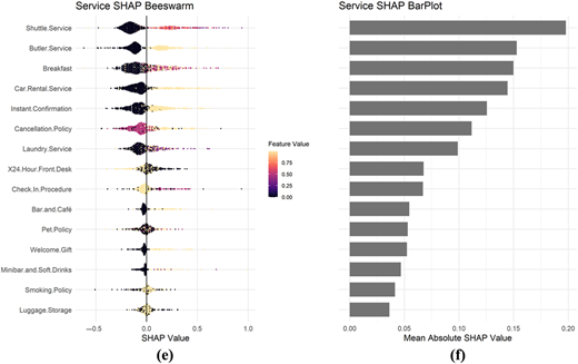
SHAP global dependence plot. Source: Authors’ own work
Graph (a): The horizontal axis is labeled “S H A P Value” and ranges from negative 0.5 to 1.5 in increments of 0.5. The vertical axis lists features in the following order: “Maximum Capacity”, “Area”, “Platform Certification Level”, “Number of Restaurants within 3 kilometers”, “Lake View”, “Floor”, “Distance to Tourist Attraction Center”, “Total Number of Reviews”, “Time Since Opening”, “Number of Tourist Attractions within 3 kilometers”, “Distance to Train Station”, “Number of Rooms”, “Service Rating”, “Facility Rating”, and “Number of Photos”. A beeswarm distribution is shown for each attribute. Each point represents an observation, and horizontal spread indicates the range of S H A P values. Point color represents feature value, ranging from low values near 0.00 to high values near 0.75 in increments of 0.25. Maximum Capacity shows the widest positive spread and highest influence, with values extending from slightly negative values to approximately 1.5. Most points cluster near negative 0.3 to 0.1, with a long positive tail. Area shows the second largest spread, ranging from approximately negative 1.4 to 0.9, with many points clustered near 0 and moderate positive values. Platform Certification Level shows strong positive effects, mostly from approximately negative 0.2 to 1.0, with many points concentrated above zero. Number of Restaurants within 3 kilometers shows moderate influence, centered near zero with spread from approximately negative 0.1 to 0.6. Lake View shows a compact distribution near zero with slight negative values up to negative 0.3. Floor shows values mostly between approximately negative 0.4 and 0.1, indicating slight negative influence overall. All the remaining shows narrow distributions concentrated close to zero, indicating relatively low influence. Graph (b): The bar graph titled “Property Attributes S H A P BarPlot” shows mean absolute S H A P values along the horizontal axis labeled “Mean Absolute S H A P Value” and ranges from 0 to 0.4 with increments of 0.1. The vertical axis lists features in the following order: “Maximum Capacity”, “Area”, “Platform Certification Level”, “Number of Restaurants within 3 kilometer”, “Lake View”, “Floor”, “Distance to Tourist Attraction Center”, “Total Number of Reviews”, “Time Since Opening”, “Number of Tourist Attractions within 3 kilometer”, “Distance to Train Station”, “Number of Rooms”, “Service Rating”, “Facility Rating”, and “Number of Photos”. The bar values are as follows. Maximum Capacity: 0.38. Area: 0.26. Platform Certification Level: 0.22. Number of Restaurants within 3 kilometers: 0.07. Lake View: 0.06. Floor: 0.05. Distance to Tourist Attraction Center: 0.045. Total Number of Reviews: 0.04. Time Since Opening: 0.038. Number of Tourist Attractions within 3 kilometers: 0.035. Distance to Train Station: 0.026. Number of Rooms: 0.026. Service Rating: 0.026. Facility Rating: 0.026. Number of Photos: 0.02. Graph (c): The horizontal axis is labeled “S H A P Value” and centers around 0, with values extending approximately from negative 0.5 to positive 0.8. The vertical axis lists features in the following order: “Swimming Pool”, “K T V”, “Kitchenware”, “Bathtub”, “Game Facilities”, “Refrigerator”, “Children s Facilities”, “Parking Lot”, “Smart Toilet”, “Conference Hall”, “Tea Room”, “Garden Terrace Courtyard”, “Smart Door Lock”, “Mahjong Parlor”, and “Heating”. Each row shows a beeswarm distribution of points, where horizontal spread indicates feature impact and color indicates feature value from low to high. Point color represents feature value, ranging from low values near 0.00 to high values near 0.75 in increments of 0.25. Swimming Pool has the strongest influence, with many positive values up to approximately 0.8 and negative values near negative 0.4. K T V is the second most influential feature, followed by Kitchenware and Bathtub, which show moderate positive effects. Game Facilities, Refrigerator, Children’s Facilities, and Parking Lot show smaller mixed effects around zero. The remaining features cluster tightly near zero, indicating low influence. Graph (d): The bar graph titled “Facility S H A P BarPlot” shows mean absolute S H A P values along the horizontal axis labeled “Mean Absolute S H A P Value” and ranges from 0 to 0.3 with increments of 0.05. The vertical axis lists features in the following order: “Swimming Pool”, “K T V”, “Kitchenware”, “Bathtub”, “Game Facilities”, “Refrigerator”, “Children s Facilities”, “Parking Lot”, “Smart Toilet”, “Conference Hall”, “Tea Room”, “Garden Terrace Courtyard”, “Smart Door Lock”, “Mahjong Parlor”, and “Heating”. The bar values are as follows. Swimming Pool: 0.355. K T V: 0.16. Kitchenware: 0.115. Bathtub: 0.08. Game Facilities: 0.07. Refrigerator: 0.065. Children s Facilities: 0.06. Parking Lot: 0.055. Smart Toilet: 0.055. Conference Hall: 0.05. Tea Room: 0.05. Garden Terrace Courtyard: 0.04. Smart Door Lock: 0.04. Mahjong Parlor: 0.035. Heating: 0.035. Graph (e): The horizontal axis is labeled “S H A P Value” and ranges approximately from negative 0.5 to 1.0 in increments of 0.5. The vertical axis lists features in the following order: “Shuttle Service”, “Butler Service”, “Breakfast”, “Car Rental Service”, “Instant Confirmation”, “Cancellation Policy”, “Laundry Service”, “24 Hour Front Desk”, “Check In Procedure”, “Bar and Cafe”, “Pet Policy”, “Welcome Gift”, “Minibar and Soft Drinks”, “Smoking Policy”, and “Luggage Storage”. Point color represents feature value, ranging from low values near 0.00 to high values near 0.75 in increments of 0.25. Each row shows a beeswarm distribution of points, where horizontal spread indicates feature impact and color indicates feature value from low to high. Shuttle Service has the strongest influence, with many positive values extending close to 1.0 and some negative values near negative 0.3. Butler Service is the second most influential feature, followed by Breakfast, Car Rental Service, and Instant Confirmation, which show moderate positive effects. Cancellation Policy and Laundry Service show mixed effects around zero with moderate spread. The remaining features cluster close to zero, indicating relatively small influence. Graph (f): The bar graph titled “Service S H A P BarPlot” shows mean absolute S H A P values along the horizontal axis labeled “Mean Absolute S H A P Value” and ranges from 0 to 0.2 with increments of 0.05. The vertical axis lists features in the following order: “Shuttle Service”, “Butler Service”, “Breakfast”, “Car Rental Service”, “Instant Confirmation”, “Cancellation Policy”, “Laundry Service”, “24 Hour Front Desk”, “Check In Procedure”, “Bar and Cafe”, “Pet Policy”, “Welcome Gift”, “Minibar and Soft Drinks”, “Smoking Policy”, and “Luggage Storage”. The bar values are as follows. Shuttle Service: 0.195. Butler Service: 0.105. Breakfast: 0.15. Car Rental Service: 0.14. Instant Confirmation: 0.125. Cancellation Policy: 0.11. Laundry Service: 0.095. 24 Hour Front Desk: 0.065. Check In Procedure: 0.066. Bar and Cafe: 0.055. Pet Policy: 0.052. Welcome Gift: 0.052. Minibar and Soft Drinks: 0.045. Smoking Policy: 0.04. Luggage Storage: 0.03. All numerical data and bar values are approximated.SHAP global dependence plot. Source: Authors’ own work
Notably, the combined contribution of Area and Maximum Capacity accounts for over 50% of the total model explanation. This aligns closely with market reality: larger space and higher guest capacity are core value drivers in the homestay sector, directly shaping consumers' willingness to pay and commanding price premiums (Mora Marquez, 2022). Additionally, Platform Certification Level emerges among the top contributors, underscoring its role as a quality signal in an information-asymmetric market. A high certification level provides a credible quality assurance to guests, significantly reducing their perceived risk and thus serving as a key basis for price formation.
The SHAP analysis further reveals that Qiandao Lake's unique locational endowment plays an irreplaceable role in price determination. The scarcity of lake view resources drives premium pricing as a dominant attraction factor. Key location-related variables – such as Lake View and Distance to Tourist Attraction Center – consistently rank among the top ten features by SHAP contribution value. This reflects the brand effect of Qiandao Lake as the “Best Waterscape under Heaven”: tourists actively seek lake-view properties to escape urban stress and immerse themselves in therapeutic natural environments. Consequently, these location-based preferences translate into rigid premium factors within the homestay pricing mechanism.
Analysis via partial dependence plots (Figure 3) confirms significant nonlinear relationships between price and key features, challenging the simplified assumptions of traditional linear models. In the case of Qiandao Lake specifically, geographic location demonstrates a distinct bimodal effect on pricing (Figure 3(a)). Within approximately one standardized distance unit from the scenic center, homestay prices decrease with increasing distance. However, beyond this standardized value, prices begin to rise again, resulting in a U-shaped relationship. This pattern likely arises from oversaturation and intense price competition among homestays close to the scenic core, driving prices downward, while more distant locations – such as mountain regions – have begun attracting high-end, tranquil homestays that leverage exclusive landscape resources, thus regaining pricing power.
 In panel (a), the vertical axis is labeled “S H A P value” and ranges from approximately negative 0.10 to 0.10 in increments of 0.05. The horizontal axis represents “Time Since Opening” and ranges from negative 2 to 1 in increments of 1. Scattered points appear in vertical clusters at several discrete horizontal values. Most points lie between approximately negative 0.06 and 0.05, with a few outliers near negative 0.10 and positive 0.08. The smooth trend line starts near approximately negative 0.07 at low values of Time Since Opening, rises steadily to positive values around the center, peaks near approximately 0.015, remains nearly flat briefly, and then declines sharply to approximately negative 0.03 at the highest values. In panel (b), the vertical axis is labeled “S H A P value” and ranges from approximately negative 0.10 to 0.10 in increments of 0.05. The horizontal axis represents “Distance to Tourist Attraction Center” and ranges from negative 1 to 3 in increments of 1. The points are widely scattered, with dense clusters between approximately negative 1 and 1 on the horizontal axis and additional sparse points extending beyond 3. Vertical values range from approximately negative 0.10 to positive 0.11. The smooth trend line starts near approximately 0.05 at the lowest distances, declines steadily below zero, reaches a minimum near approximately negative 0.045 around mid to higher distances, and then rises again to positive values above 0.06 at the farthest distances. Note: All numerical values are approximated.
Partial dependence plots of distance to scenic center (a) and Years Since Opening (b). Source: Authors’ own work
In panel (a), the vertical axis is labeled “S H A P value” and ranges from approximately negative 0.10 to 0.10 in increments of 0.05. The horizontal axis represents “Time Since Opening” and ranges from negative 2 to 1 in increments of 1. Scattered points appear in vertical clusters at several discrete horizontal values. Most points lie between approximately negative 0.06 and 0.05, with a few outliers near negative 0.10 and positive 0.08. The smooth trend line starts near approximately negative 0.07 at low values of Time Since Opening, rises steadily to positive values around the center, peaks near approximately 0.015, remains nearly flat briefly, and then declines sharply to approximately negative 0.03 at the highest values. In panel (b), the vertical axis is labeled “S H A P value” and ranges from approximately negative 0.10 to 0.10 in increments of 0.05. The horizontal axis represents “Distance to Tourist Attraction Center” and ranges from negative 1 to 3 in increments of 1. The points are widely scattered, with dense clusters between approximately negative 1 and 1 on the horizontal axis and additional sparse points extending beyond 3. Vertical values range from approximately negative 0.10 to positive 0.11. The smooth trend line starts near approximately 0.05 at the lowest distances, declines steadily below zero, reaches a minimum near approximately negative 0.045 around mid to higher distances, and then rises again to positive values above 0.06 at the farthest distances. Note: All numerical values are approximated.Partial dependence plots of distance to scenic center (a) and Years Since Opening (b). Source: Authors’ own work
Moreover, Time Since Opening shows an inverted U-shaped relationship with price, with homestay prices peaking around the third year of operation and then gradually declining (Figure 3(b)). This finding contradicts the simplistic notion that “newer properties can always charge more,” and instead aligns with classic product life cycle theory. A dynamic, game-theoretic interpretation is as follows: during the market entry phase (0–1 year), new homestays often employ low introductory pricing (penetration pricing) to quickly attract guests and build a reputation. In the growth and maturity phase (about 2–4 years), established homestays enhance their offerings (through facility upgrades and service standardization) and capitalize on accumulated positive review, which allows them to command higher prices. Finally, in the decline phase (5+ years), aging properties and amenities lead to decreased appeal and competitive pricing pressure, eroding price premiums. These nonlinear pricing dynamics illustrate the evolving value trajectory of homestay products over their life cycle.
5. Construction and validation of comprehensive facility and service indicators
5.1 Construction of comprehensive facility and service indicators
In much of the homestay pricing literature, facilities are encoded as undifferentiated binary variables. As a result, prevalence effects can dilute the marginal impact of rare, high-valuation features and obscure heterogeneity in willingness to pay. We address this issue by constructing two composite measures – Facility Index (FI) and Service Index (SI) – that use SHAP-based, data-driven weights estimated within the modeling framework. These indices aggregate amenity information while preserving differential contributions and reducing sparsity, thereby relaxing the equal-weight assumption that underlies many existing specifications. The resulting measures offer a parsimonious, comparable and economically interpretable representation of amenity quality across listings.
5.1.1 Target encoding and feature optimization
Given the discrete and multidimensional nature of facility and service features, we use target encoding to obtain a more informative numerical representation. Raw facility values follow an ordinal scheme (0 = none, 1 = free, 2 = partially charged, 3 = fully charged). However, naïve ordinal coding cannot capture nonlinear price responses across these categories.
We therefore split the data into a 75% training set and a 25% test set, and implement five-fold out-of-fold target encoding (K = 5, α = 10) within the training data. For each fold, encoding values are computed using only the remaining training folds, combining category-specific means with the global mean via Bayesian smoothing. The resulting encodings are then applied to the held-out fold and to the test set using training-set statistics only, thereby preventing information leakage.
: The target encoding value of the feature .
: The mean of feature (category mean).
: The number of samples for feature .
: The global mean of the feature variable across the entire dataset.
: The smoothing coefficient, used to balance the category mean and the global mean's weight.
For the hold-out test set, encoding values were strictly derived from the global statistics of the training set. Importantly, we retained the original state for categories with zero values, minimizing noise and preventing information leakage. This encoding scheme thus ensures robust numerical representations of categorical features, enhances feature stability and preserves the integrity of the evaluation by eliminating any influence from the test data.
5.1.2 Construction of comprehensive indicators
To quantify the dynamic impact of facilities and services on pricing, we adopted a stepwise modeling strategy. We first incorporated facility configuration features into the XGBoost model and identified the top 15 facility-related features by their SHAP importance. Separately, we incorporated service management features and identified the top 15 service-related features by SHAP importance. We then extracted each selected feature's mean Shapley value. By evaluating facilities and services in separate runs, we avoided the situation where dominant property attributes might overshadow the contribution of any single facility or service feature, thus obtaining a clearer picture of amenity impacts.
Using these SHAP results, we constructed two composite indices to summarize the contribution of facilities and services, respectively. Essentially, each composite index is a weighted sum of the presence (encoded value) of the top features, using their SHAP contributions as weights. Formally, for the Facility Index (FI)/ Service Index (SI):
: The target encoded value of the th feature in the facility configuration.
: The target encoded value of the th feature in the service management.
: The Shapley value of the th feature.
This weighting means that features with larger positive contributions raise the index more, while those with negative impacts lower the index accordingly.
The facility-only SHAP (Figure 2(c) and 2(d)) analysis provides insight into which amenities most strongly drive prices. Having a swimming pool yields the highest SHAP value (∼+0.34), indicating it contributes substantially to the price premium. Following that, entertainment amenities such as KTV and Mahjong parlor also show notable positive impacts on price. Additionally, the configuration of kitchenware and refrigerator supports the long-term rental demand for homestays, enhances a property's appeal and can increase its price.
In the service-only SHAP results (Figure 2(e) and 2(f)), offering a Shuttle Service (transportation for guests) has the strongest positive effect on price among services. This makes sense in our context: although a public shuttle connects the area to Qiandao Lake Station, homestays are scattered and often remote, so a dedicated Shuttle Service adds significant convenience/value. A butler service also considerably improves the guest experience and thus commands a price premium.
With dozens of features in play, analyzing each individually would be cumbersome and could introduce redundancy. To simplify further analysis, we therefore use the comprehensive indices (FI and SI) that we computed by aggregating the top features' contributions. In the next section, we reintroduce these composite indices into the model to evaluate their effects in combination with the core property attributes.
5.2 Interaction effects and marginal impact analysis
Incorporating FI and SI alongside property attributes markedly improves fit (R2 = 0.893) and reduces errors (RMSE = 0.341; MAE = 0.214), indicating that the aggregated amenity signal mitigates redundancy among individual features and captures synergistic effects more succinctly than a long list of stand-alone dummies.
In the updated SHAP-based global importance ranking, the FI ranks third, following Maximum Capacity, while the SI ranks fifth, just below Platform Certification Level. Their combined contribution surpasses that of any single traditional attribute, underscoring that aggregated facilities and services exert an independent, substantial influence on pricing. This affirms our methodology: rather than mere add-ons, superior facility and service quality can rival or exceed core property traits in explaining price variations.
SHAP waterfall plots offer per-listing diagnostics that support actionable managerial decisions. Figure 4 presents the waterfall for a median-scenario listing, decomposing the predicted price into additive feature contributions: a binding capacity constraint exerts a sizeable negative effect (SHAP = −0.275), partially offset by a high Service Index (+0.171). These contributions suggest that increasing the platform certification tier and, where feasible, expanding maximum capacity would generate additional price uplift. Extending the same procedure to other representative profiles yields tailored, rank-ordered recommendations on which managerial levers – capacity expansion, service upgrades or facility additions – are expected to deliver the largest marginal price gains, subject to cost and operational constraints.
 The waterfall chart titled “SHAP Waterfall plot — Median Sample” shows feature contributions along the horizontal axis labeled “Prediction” ranging from 6.0 to 6.2 with increments of 0.1. The vertical axis lists features in the following order: “Maximum Capacity equals negative 0.715”, “Service Index equals 5.82”, “Platform Certification Level equals 2”, “Lake View equals 1”, “22 other features”, “Floor equals 0.809”, “Area equals 0.148”, “Number of Restaurants within 3 kilometers equals 0.901”, “Number of Tourist Attractions within 3 kilometers equals 1.55”, and “Service Rating equals 0.535”. Each horizontal bar represents the contribution of a feature to the prediction value, with positive contributions extending toward higher prediction values and negative contributions extending toward lower values. The contribution values are as follows. Maximum Capacity equals negative 0.275. Service Index equals positive 0.171. Platform Certification Level equals negative 0.0967. Lake View equals positive 0.0927. 22 other features equals positive 0.0902. Floor equals negative 0.0858. Area equals positive 0.0719. Number of Restaurants within 3 kilometers equals negative 0.0408. Number of Tourist Attractions within 3 kilometers equals negative 0.0345. Service Rating equals positive 0.0327. The cumulative effect of these contributions results in a final prediction value near 6.2.
SHAP waterfall plot for median-priced homestay Sample. Source: Authors’ own work
The waterfall chart titled “SHAP Waterfall plot — Median Sample” shows feature contributions along the horizontal axis labeled “Prediction” ranging from 6.0 to 6.2 with increments of 0.1. The vertical axis lists features in the following order: “Maximum Capacity equals negative 0.715”, “Service Index equals 5.82”, “Platform Certification Level equals 2”, “Lake View equals 1”, “22 other features”, “Floor equals 0.809”, “Area equals 0.148”, “Number of Restaurants within 3 kilometers equals 0.901”, “Number of Tourist Attractions within 3 kilometers equals 1.55”, and “Service Rating equals 0.535”. Each horizontal bar represents the contribution of a feature to the prediction value, with positive contributions extending toward higher prediction values and negative contributions extending toward lower values. The contribution values are as follows. Maximum Capacity equals negative 0.275. Service Index equals positive 0.171. Platform Certification Level equals negative 0.0967. Lake View equals positive 0.0927. 22 other features equals positive 0.0902. Floor equals negative 0.0858. Area equals positive 0.0719. Number of Restaurants within 3 kilometers equals negative 0.0408. Number of Tourist Attractions within 3 kilometers equals negative 0.0345. Service Rating equals positive 0.0327. The cumulative effect of these contributions results in a final prediction value near 6.2.SHAP waterfall plot for median-priced homestay Sample. Source: Authors’ own work
We further analyzed the joint impact of Platform Certification Level and Total Number of Reviews on pricing (Figure 5(a)). For low-rated homestays, additional reviews exert a robust positive effect, enhancing consumer confidence by reducing information asymmetry around subpar listings. Conversely, high-rated homestays exhibit diminishing returns from more reviews, potentially turning negative at extremes; with established quality, extra feedback adds minimal value and may arouse skepticism about authenticity. This reveals a subtle risk-aversion dynamic in consumer behavior: reviews potently alleviate uncertainty in low-quality scenarios but offer limited benefits – and possible drawbacks – when quality is already assured.
 Panel (a): Platform Certification Level S H A P Dependence. The horizontal axis is labeled “Platform Certification Level” and ranges from 0 to 5 in increments of 1. The vertical axis is labeled “S H A P value” and ranges from negative 0.50 to 0.50 in increments of 0.25. Points appear in vertical clusters at discrete certification levels. Lower levels around 0 to 2 are mostly negative, centered near approximately negative 0.15. Higher levels around 3 to 4 are strongly positive, reaching approximately 0.45. Point color represents Total Number of Reviews, which ranges from negative 1 to 2 in increments of 1 unit. Panel (b): Lake View S H A P Dependence. The horizontal axis is labeled “Lake View” with binary values 0 and 1. The vertical axis is labeled “S H A P value” and ranges approximately from negative 0.1 to 0.1 in increments of 0.1. Two vertical clusters are shown. Lake View equals 0 is centered slightly below zero, while Lake View equals 1 is centered clearly above zero, with values reaching approximately 0.12. Point color represents Area which ranges from negative 1 to 2 in increments of 1 unit. Panel (c): Facility Index S H A P Dependence. The horizontal axis is labeled “Facility Index” and ranges from approximately 2.5 to 10 in increments of 2.5. The vertical axis is labeled “S H A P value” and ranges from negative 0.50 to 0.50 in increments of 0.25. A scatter distribution with a smooth curve is shown. The trend curve rises from approximately negative 0.20 at low index values, crosses above zero near approximately 3, peaks near approximately 0.26 around 7, and then declines slightly toward approximately 0.10 near 10. Data points are scattered around the trend curve. Point color represents Service Index, which ranges from 2.5 to 7.5 in increments of 2.5 units. Panel (d): Area- Facility Index S H A P 2 D Dependence. The horizontal axis is labeled “Area” and ranges from approximately negative 1 to 2 in increments of 1. The vertical axis is labeled “Facility Index” and ranges from 0 to 10 in increments of 2.5. Points are colored by S H A P value. Lower area and lower facility index regions show darker colors, indicating lower S H A P values. Higher area and higher facility index regions show warmer colors, indicating higher S H A P values, with the strongest values concentrated in the upper right region. Data point color represents S H A P values, which ranges from negative 0.4 to 1.22 in increments of 0.4 units. Note: All numerical values are approximated.
Combined SHAP dependence plots. Source: Authors’ own work
Panel (a): Platform Certification Level S H A P Dependence. The horizontal axis is labeled “Platform Certification Level” and ranges from 0 to 5 in increments of 1. The vertical axis is labeled “S H A P value” and ranges from negative 0.50 to 0.50 in increments of 0.25. Points appear in vertical clusters at discrete certification levels. Lower levels around 0 to 2 are mostly negative, centered near approximately negative 0.15. Higher levels around 3 to 4 are strongly positive, reaching approximately 0.45. Point color represents Total Number of Reviews, which ranges from negative 1 to 2 in increments of 1 unit. Panel (b): Lake View S H A P Dependence. The horizontal axis is labeled “Lake View” with binary values 0 and 1. The vertical axis is labeled “S H A P value” and ranges approximately from negative 0.1 to 0.1 in increments of 0.1. Two vertical clusters are shown. Lake View equals 0 is centered slightly below zero, while Lake View equals 1 is centered clearly above zero, with values reaching approximately 0.12. Point color represents Area which ranges from negative 1 to 2 in increments of 1 unit. Panel (c): Facility Index S H A P Dependence. The horizontal axis is labeled “Facility Index” and ranges from approximately 2.5 to 10 in increments of 2.5. The vertical axis is labeled “S H A P value” and ranges from negative 0.50 to 0.50 in increments of 0.25. A scatter distribution with a smooth curve is shown. The trend curve rises from approximately negative 0.20 at low index values, crosses above zero near approximately 3, peaks near approximately 0.26 around 7, and then declines slightly toward approximately 0.10 near 10. Data points are scattered around the trend curve. Point color represents Service Index, which ranges from 2.5 to 7.5 in increments of 2.5 units. Panel (d): Area- Facility Index S H A P 2 D Dependence. The horizontal axis is labeled “Area” and ranges from approximately negative 1 to 2 in increments of 1. The vertical axis is labeled “Facility Index” and ranges from 0 to 10 in increments of 2.5. Points are colored by S H A P value. Lower area and lower facility index regions show darker colors, indicating lower S H A P values. Higher area and higher facility index regions show warmer colors, indicating higher S H A P values, with the strongest values concentrated in the upper right region. Data point color represents S H A P values, which ranges from negative 0.4 to 1.22 in increments of 0.4 units. Note: All numerical values are approximated.Combined SHAP dependence plots. Source: Authors’ own work
Our interaction analysis shows that property size meaningfully shapes the value of specific amenities, with particularly strong effects for lake views and facility bundles. As shown in Figure 5(b), small-area homestays cluster in regions of the feature space where the Lake View attribute has substantially higher SHAP values, whereas larger properties exhibit much weaker lake-view contributions to price. For compact homestays, a lake view can therefore become the focal element of the guest experience and be monetized more fully. By contrast, larger properties typically offer multiple competing amenities (e.g. courtyards, KTV rooms), which dilute the relative contribution of any single feature such as a lake view. Because small units also start from a lower base price, the same scenic resource generates a larger proportional uplift, leading to a steeper marginal price increase. Taken together, these patterns indicate a size-dependent efficiency in converting scenic resources into revenue: compact designs are more effective at transforming a single visual advantage into economic value.
Building on this, Figure 5(c) documents diminishing marginal returns to facility and service quality. When the Facility Index (FI) is below roughly 5, prices rise almost linearly with each additional facility, indicating consistent value gains. Beyond this threshold, however, further increases in FI are associated with much flatter SHAP curves, even when the Service Index (SI) continues to grow. In other words, amenity additions initially enhance perceived value, but once saturation is reached, the pricing benefits taper off. This pattern is particularly salient for larger properties, which typically start with higher FI values and thus reach the plateau earlier. For such listings, continued investment in low-utilization or redundant amenities is unlikely to generate commensurate price increases, underscoring the need for strategic restraint in further amenity expansion.
This interpretation is supported by Figure 5(d), which specifically illustrates how the marginal returns of facility enhancements differ by property size. For small-area homestays (Area <0.5), an increase in FI is accompanied by a clear lightning of color in the scatter plot, representing higher SHAP values. This reflects strong incremental pricing benefits from facility upgrades. In contrast, for properties with Area >0.5, this color gradient is far less pronounced, indicating that once a property already has a comprehensive set of amenities, the marginal benefit of adding more diminishes rapidly. In essence, guests may not value or use additional features beyond a certain point, particularly in spacious properties where amenities become functionally substitutable or less visible. This insight has practical implications: investment decisions in amenity improvements should be tailored to the physical constraints and market positioning of the property.
6. Robustness test
To ensure the robustness of the main model's conclusion, we conducted tests from two aspects: sample extrapolation and method substitution.
6.1 New sample extrapolation test
At Qiandao Lake, the peak season typically spans late summer through autumn; September remains a period of high demand with elevated prices. To assess cross-season generalization, we apply the trained XGBoost – SHAP pipeline to an adjacent peak-season window (September 5–6) without any change to the baseline workflow. We collected valid information for 3,074 rooms; after excluding listings with missing prices and those duplicated relative to the baseline, 678 samples remained for evaluation. Because a few variables could not be consistently retrieved due to page-scraping constraints, we omitted those variables to maintain measurement consistency; the definitions and computation of the “Facility Index” and “Service Index” remained unchanged. The baseline log transformation and z-score standardization were retained.
Because raw September prices are higher on average, we first re-level the predicted September prices using the cross-season mean ratio. This step aligns average price levels across seasons before evaluation and affects only the mean, not higher-order moments such as variance or distributional shape. We then report both absolute-scale metrics (RMSE, MAE, R2) and relative-scale metrics (MAE%, nRMSE with respect to the mean, SMAPE). Relative to the baseline season, extrapolation to September produces a moderate decline in performance: R2 decreases from 0.893 to 0.767, RMSE increases from 0.341 to 0.498, and MAE rises from 0.214 to 0.406. In absolute terms, errors are larger in the peak season, but in relative terms, the increases are modest. Taken together, these results suggest that, after mean re-leveling, higher absolute errors are driven primarily by greater dispersion in peak-season prices and covariate shift in the feature distribution, rather than by residual level differences or structural misfit. Recomputing SHAP values on the September sample yields global feature importance rankings that are highly consistent with the baseline: “Maximum Capacity,” “Area,” “Facility Index,” “Platform Certification Level,” “Floor” and “Service Index” remain the top six contributors. This corroborates the stability of the underlying pricing mechanism across seasons.
6.2 Generalized additive model substitution test
To cross-validate the main conclusion from a statistical inference perspective, we re-estimated the original sample using GAM. XGBoost is convenient for handling high-dimensional features and providing individual-level interpretability; GAM provides parametric significance tests and confidence intervals. The two complement each other, simultaneously covering the prediction and interpretation dimensions, and enhance the credibility of the conclusion through result consistency.
We estimate a GAM that includes fixed effects for categorical variables such as Lake View and Platform Certification Level, and smooth terms for key continuous variables such as Time Since Opening, Facility Index, and Distance to Tourist Attraction Center. Restricted maximum likelihood (REML) is used to select the degree of smoothness. The basis dimension k for each smooth term is set according to the diversity of observed values (approximately 4–10), and selective shrinkage is applied to weaken redundant or approximately linear components. The GAM fits the data well: the adjusted R2 is 0.841, the deviance explained is 84.6%, and the AIC is 3436.757 (n = 3,054). The smooth terms are jointly significant at the 1% level, indicating a statistically significant nonlinear response of prices to the corresponding factors (Table 2). The relative importance measured by F-statistics is largely consistent with the global ranking of SHAP values. The importance of the Facility Index further increases, while that of the Service Index decreases slightly, without changing the core conclusion. Maximum Capacity, Facility Index, Area and Floor exhibit pronounced nonlinear curve effects, whereas Facility Rating and Number of Photos have effective degrees of freedom (EDF) close to 1, so their nonlinear components are shrunk toward approximate linearity. Residual diagnostics show no serious non-normality, heteroscedasticity or systematic bias, supporting the adequacy of the model specification.
GAM significance test results
| Variable | EDF (effective df) | F-value | p-value | Significance | k-index | p-value (k-check) |
|---|---|---|---|---|---|---|
| Maximum Capacity | 5.6218417 | 46.364086 | 0 | *** | 0.75 | <2e-16 |
| Facility Index | 5.147798 | 28.48155 | 0 | *** | 0.79 | <2e-16 |
| Area | 2.3031761 | 16.254806 | 0 | *** | 0.83 | <2e-16 |
| Floor | 4.6486023 | 13.608813 | 0 | *** | 0.81 | <2e-16 |
| Number of Restaurants within 3 km | 7.0945884 | 11.950357 | 0 | *** | 0.71 | <2e-16 |
| Distance to Tourist Attraction Center | 5.8894908 | 10.049402 | 0 | *** | 0.71 | <2e-16 |
| Total Number of Reviews | 6.9468622 | 7.602804 | 0 | *** | 0.72 | <2e-16 |
| Time Since Renovation | 6.8056748 | 5.774508 | 0 | *** | 0.71 | <2e-16 |
| Recommendation Percentage | 5.5398729 | 4.824016 | 0 | *** | 0.7 | <2e-16 |
| Number of Tourist Attractions within 3 km | 4.126531 | 4.168717 | 0 | *** | 0.72 | <2e-16 |
| Number of Shops within 3 km | 2.7614318 | 4.16267 | 0 | *** | 0.71 | <2e-16 |
| Distance to Train Station | 6.2482676 | 3.744644 | 6.406996e-07 | *** | 0.69 | <2e-16 |
| Environmental Rating | 4.7579637 | 3.437259 | 6.7116e-08 | *** | 0.68 | <2e-16 |
| Service Index | 2.5784371 | 3.394732 | 0 | *** | 0.82 | <2e-16 |
| Time Since Opening | 4.0094266 | 3.187548 | 1.3202e-06 | *** | 0.71 | <2e-16 |
| Cleanliness Rating | 5.4888692 | 3.111862 | 2.589561e-06 | *** | 0.71 | <2e-16 |
| Facility Rating | 0.9740422 | 2.502365 | 7.510555e-07 | *** | 0.7 | <2e-16 |
| Number of Photos | 0.9564811 | 2.199897 | 4.551813e-06 | *** | 0.93 | <2e-16 |
| Service Rating | 2.828162 | 1.865738 | 8.682243e-05 | *** | 0.7 | <2e-16 |
| Number of Rooms | 2.5330802 | 1.003599 | 0.007833138 | ** | 0.72 | <2e-16 |
In terms of the rationality of “k,” the EDF of most variables do not approach the upper limit, and only a few variables are close to the upper limit, suggesting that the flexibility may be insufficient. Further implementing adaptive smoothing on key variables shows that: the adaptive curve of “Time Since Opening” is consistent with the baseline model, and its main turning point position is consistent with the SHAP dependency graph (Figure 6(a)); the overall trend of “Distance to Tourist Attraction Center” is similar, with more obvious curvature in the middle section, presenting an approximately “W” shape trend, but the confidence band of this interval is wide and the statistical significance is limited (Figure 6(b)); the partial effect of “Facility Index” shows a clearer marginal diminishing feature, and the curve has a turning point around index 4–5 (Figure 6(c)). In addition, we also generated the three-dimensional interaction between Area and FI for comparison (Figure 6(d)).Overall, GAM is consistent with XGBoost- SHAP in variable ranking, main effect shape and threshold interval, further supporting the robustness and reproducibility of the main conclusion of this article from the methodological perspective.
 Panel (a): Time Since Opening: The horizontal axis is labeled “Time Since Opening” and ranges from approximately negative 5 to 1 in increments of 1. The vertical axis is labeled “Partial effect” and ranges from approximately negative 0.3 to 0.2 in increments of 0.1. Two curves are shown: Baseline and Adaptive, with a shaded 95 percent confidence interval. Both curves rise from negative values at low x values, peak near approximately 0.18 around negative 1, then decline sharply after 0 and reach below negative 0.30 near 1.3. The two curves closely overlap. Panel (b): Distance to Tourist Attraction Center: The horizontal axis is labeled “Distance to Tourist Attraction Center” and ranges from approximately negative 1 to 3 in increments of 1. The vertical axis is labeled “Partial effect” and ranges from approximately negative 0.1 to 0.3 in increments of 0.1. Both curves begin high near approximately 0.34, fall below negative 0.1 near 0, remain negative, rise to a positive bump near 2, dip again near 2.8, and rise toward the far right. The adaptive confidence interval widens at the extremes. Panel (c): Facility Index: The horizontal axis is labeled “Facility Index” and ranges from 0 to 10 in increments of 2. The vertical axis is labeled “Partial effect” and ranges from approximately negative 0.2 to 0.3 in increments of 0.1. Both curves increase steadily from approximately negative 0.28 at low values, cross zero near 2.3, rise rapidly to about 0.20 near 4, then continue gradual growth and level near approximately 0.28 by 9 to 10. The two curves nearly coincide. Panel (d): Facility Index - Area Interaction Effect Plot: A three-dimensional surface plot is shown. The horizontal axes are labeled “Facility Index” and “Area”. The “Facility Index” axis ranges from 0 to 8 in increments of 2. The “Area” axis ranges from negative 2 to 2 in increments of 1. The vertical axis is labeled “Linear predictor” and ranges from 4.0 to 6.0 in increments of 0.5. The surface rises overall from lower values at low facility index and low area toward higher values at larger facility index and area, with visible ridges and shallow valleys indicating nonlinear interaction patterns. Note: All numerical values are approximated.
Gam partial effect plot. Source: Authors’ own work
Panel (a): Time Since Opening: The horizontal axis is labeled “Time Since Opening” and ranges from approximately negative 5 to 1 in increments of 1. The vertical axis is labeled “Partial effect” and ranges from approximately negative 0.3 to 0.2 in increments of 0.1. Two curves are shown: Baseline and Adaptive, with a shaded 95 percent confidence interval. Both curves rise from negative values at low x values, peak near approximately 0.18 around negative 1, then decline sharply after 0 and reach below negative 0.30 near 1.3. The two curves closely overlap. Panel (b): Distance to Tourist Attraction Center: The horizontal axis is labeled “Distance to Tourist Attraction Center” and ranges from approximately negative 1 to 3 in increments of 1. The vertical axis is labeled “Partial effect” and ranges from approximately negative 0.1 to 0.3 in increments of 0.1. Both curves begin high near approximately 0.34, fall below negative 0.1 near 0, remain negative, rise to a positive bump near 2, dip again near 2.8, and rise toward the far right. The adaptive confidence interval widens at the extremes. Panel (c): Facility Index: The horizontal axis is labeled “Facility Index” and ranges from 0 to 10 in increments of 2. The vertical axis is labeled “Partial effect” and ranges from approximately negative 0.2 to 0.3 in increments of 0.1. Both curves increase steadily from approximately negative 0.28 at low values, cross zero near 2.3, rise rapidly to about 0.20 near 4, then continue gradual growth and level near approximately 0.28 by 9 to 10. The two curves nearly coincide. Panel (d): Facility Index - Area Interaction Effect Plot: A three-dimensional surface plot is shown. The horizontal axes are labeled “Facility Index” and “Area”. The “Facility Index” axis ranges from 0 to 8 in increments of 2. The “Area” axis ranges from negative 2 to 2 in increments of 1. The vertical axis is labeled “Linear predictor” and ranges from 4.0 to 6.0 in increments of 0.5. The surface rises overall from lower values at low facility index and low area toward higher values at larger facility index and area, with visible ridges and shallow valleys indicating nonlinear interaction patterns. Note: All numerical values are approximated.Gam partial effect plot. Source: Authors’ own work
7. Discussion and conclusions
7.1 Conclusions
This study investigates homestay pricing in the Qiandao Lake region by embedding machine-learning models within an explainable AI (XAI) framework. Using a three-tier feature system that covers property attributes, facility configurations and service characteristics, we show how these elements jointly shape price formation at the listing level.
First, compared with conventional hedonic pricing models, the proposed approach more precisely quantifies the effects of facilities and services and captures important nonlinear price responses. SHAP-based local explanations reveal interaction patterns that static coefficients would miss. Prices exhibit a bimodal spatial pattern, with a second premium peak in less congested scenic areas where landscape resources (lake and mountain views) support a “healing” premium. We also identify an inverted-U life cycle: new listings discount to build reputation and market share, whereas established ones place more weight on revenue per guest.
Second, to address the high-dimensional and discrete structure of amenity variables, we construct SHAP-based composite indicators of facilities (FI) and services (SI). These indices aggregate amenities with data-driven weights, reduce dimensionality and multicollinearity, and explain price variation better than individual attributes. Facilities and services influence pricing through nonlinear interactions and threshold effects consistent with diminishing marginal returns.
Third, cross-season extrapolation and a complementary GAM re-estimation indicate that the main pricing mechanisms and the FI/SI hierarchy are robust across demand regimes and modeling choices. The Facility Index, Service Index and core attribute effects remain broadly stable and transferable beyond the baseline sample.
7.2 Theoretical implications
This study contributes to pricing research at the intersection of hedonic theory, tourism economics and machine learning in two main ways.
First, it helps to narrow the gap between predictive accuracy and interpretability by integrating XGBoost with SHAP explanations within a hedonic logic. Rather than treating machine-learning models as black boxes, we show how local contribution profiles can be interpreted in terms of marginal effects, diminishing returns and interaction patterns, thereby linking XAI outputs back to familiar economic concepts.
Second, the SHAP-based Facility and Service Indices provide an operational bridge between traditional attribute-based hedonic models and aggregated amenity constructs. Unlike ad hoc or equal-weight indices, FI and SI are grounded in model-implied marginal contributions and offer an empirically driven way to summarize complex amenity structures. Combined with the evidence on bimodal spatial patterns, life-cycle dynamics and segment-specific bundle valuations, this supports a more dynamic and segmentation-sensitive view of homestay pricing than static average-effect models.
7.3 Practical implications
The findings also yield implications for homestay operators, platforms and destination managers.
For individual hosts and property managers, FI and SI translate complex model outputs into practical levers. When FI is low, selectively adding a small set of high-impact amenities generates the largest marginal gains. As FI approaches an empirically observed saturation range, returns to additional facilities diminish and resources are better directed toward service upgrades, pricing refinement and targeted marketing. Property size matters: in compact listings, scenic features and focused service bundles monetize strongly, whereas in larger properties the marginal payoff of “more of everything” is weaker, so avoiding over-investment in redundant facilities is important. Per-listing SHAP waterfalls further indicate whether capacity, facilities or services move the price most for a specific property, enabling sequenced budgeting and more transparent ROI assessments.
For platforms and destination managers, FI and SI can serve as benchmarking tools for monitoring homestay quality, identifying under- or over-supplied amenity bundles and anticipating price pressures in environmentally sensitive or congested zones. Regulators and DMOs can use these indices to design differentiated standards and incentive schemes that encourage high-value amenities and service enhancements, rather than uniform expansion of facility sets. Aligning infrastructure provision, certification and support policies with data-driven evidence on what guests value can improve both market efficiency and the sustainability of local development.
7.4 Limitations and future research
Despite the contributions, two limitations remain. First, the dataset lacks granular demand-side information, so heterogeneity is inferred indirectly from prices and reviews. Second, results are based on a single destination, which may limit generalizability to markets with different structures or regulations. Future research could enrich the FI/SI framework by integrating multimodal signals and by combining high-frequency booking/occupancy data with systematic competitor price tracking or simulation-based designs to better model traveler decisions and local competitive dynamics.
The author gratefully acknowledges the support of the National Natural Science Foundation of China (award number: 42171243).

