Lateral stability regulation of intelligent electric vehicle based on model predictive control

Li, Cong; Xie, YunFeng; Wang, Gang; Zeng, XianFeng; Jing, Hui

doi:10.1108/JICV-03-2021-0005

Purpose

This paper studies the lateral stability regulation of intelligent electric vehicle (EV) based on model predictive control (MPC) algorithm.

Design/methodology/approach

Firstly, the bicycle model is adopted in the system modelling process. To improve the accuracy, the lateral stiffness of front and rear tire is estimated using the real-time yaw rate acceleration and lateral acceleration of the vehicle based on the vehicle dynamics. Then the constraint of input and output in the model predictive controller is designed. Soft constraints on the lateral speed of the vehicle are designed to guarantee the solved persistent feasibility and enforce the vehicle’s sideslip angle within a safety range.

Findings

The simulation results show that the proposed lateral stability controller based on the MPC algorithm can improve the handling and stability performance of the vehicle under complex working conditions.

Originality/value

The MPC schema and the objective function are established. The integrated active front steering/direct yaw moments control strategy is simultaneously adopted in the model. The vehicle’s sideslip angle is chosen as the constraint and is controlled in stable range. The online estimation of tire stiffness is performed. The vehicle’s lateral acceleration and the yaw rate acceleration are modelled into the two-degree-of-freedom equation to solve the tire cornering stiffness in real time. This can ensure the accuracy of model.

1. Introduction

With the rapid increasing demands on vehicle quality, modern car makers are paying more attention on improving vehicle safety issue. Thanks to the evolution of the electronic and information technology, many advanced techniques can be applied to the intelligent vehicles, such as autonomous emergency braking and electronic stabilization programs (ESP), to enhance the safety issue. Thus, the vehicle quality can be improved and safety issue can be guaranteed, and then the traffic accident can be reduced (Liu et al., 2020; Xiao et al., 2021; Xu et al., ,2020; Lyckegaard et al., ,2015). Electric vehicle (EV), which has lower carbon emission, is an important industry in the world. Four-wheel independently driving electric vehicle (FWID-EV), equipped with in-wheel motors, is a promising EV architecture. As the characteristic of fast response and high accuracy, these intelligent and safety techniques can be realized and the traffic accidents can be effectively reduced. Lateral stability control of EV is critical to the handling and stability performance of EVs, thus is attached many interests from academics and industry (Jiang et al., 2020; Mangia et al., 2021; Zhao and Zhang, 2018; Xue et al., ,2019; Guo et al., ,2019; Ni et al., ,2019; Cao et al., 2020).

Vehicle’s stability can be regulated by direct yaw moments control (DYC). The ESP system changes the vehicle direct yaw moments and keeps the vehicle in the stable state by controlling the longitudinal force of the tire (Geng et al., 2009; Jalali et al., 2018; Wang et al., ,2014). If the inertial sensor detects the vehicle in oversteering state, the outer wheels of the vehicle are braked to reduce the longitudinal force on the tire, then the sideslip angle of the vehicle is controlled in the stable range. On the contrary, when the understeering is detected, the inner wheels of the vehicle are braked to enhance the yaw moment and improve the handling and stability performance. The active front steering (AFS) is another way to stabilize the vehicle (Guo et al., 2018; Poussot-Vassal et al., 2011). Reference (Nam et al., 2012) presents a robust yaw stability control based on the AFS control for the four-wheel independently driving EV; however, when the lateral tire force is saturated the AFS control will fail to regulate the vehicle. Yang et al. (2009) presents a controller based on optimal guaranteed cost theory, where the controller coordinates the front steering and DYC and consider the uncertainties of tire cornering stiffness. Zhang et al. (2016) study the observer design problem for polytopic linear-parameter-varying systems with uncertain measurements on scheduling variables. Tjonnas and Johansen (2010) present a multi-level modular control structure for indirect sideslip angle and yaw rate tracking control, and the yaw moments allocation control is casted as dynamic optimization. Ni et al. (2017) investigate an envelope controller which integrate the AFS and DYC. Zhao et al. (2018) consider a weighted function to express the uncertain system the parameters, uncertainties of vehicle speed and tire cornering stiffness and then gives μ controller to track the desired sideslip angle and yaw rate. Ren et al. (2016) present a model predictive controller based on the holistic control structure through AFS and motor torque distribution, where the nonlinear characteristics of each tire force between tire and road and input maximum torque of the driving motor are considered. In Peng et al. (2020), the path tracking and direct yaw moment coordinated control based on robust model predictive control (MPC) with the finite time horizon for autonomous independent drive vehicles is studied. Lin et al. (2019) investigate the trajectory tracking with the fusion of DYC and longitudinal-lateral control method for autonomous vehicle. Zhang et al. (2020) evaluate model predictive path following and yaw stability controllers for over-actuated autonomous EVs is given. The integrated control AFS/DYC is effective to enhance the handling and stability performance in aforementioned literatures.

However, there have several points to be improved as follows:

The handling and stability performance of the vehicle control requires fast regulation in real application. Considering the computation ability of the real-time processor, the performance of the above control system might be degraded.
Many parameters of the Magic Formula model of the tire must be tested under massive experiment tests in the works, i.e. the calculation of lateral and longitudinal stiffness of tires are very complicated and time-consuming.

In addition, the sideslip angle of vehicle and tires longitudinal slip ratio are supposed to be known in the related works, which is a relative hard task in real application.

The advantage of the FWID-EV is that the torque of in-wheel motor can quickly respond to the commands and the torque can be controlled accurately and independently (Hori, 2014). Therefore, the handling and stability performance of the vehicle using AFS and DYC can be effective. The main contributions of this paper are as follows:

Based on the bicycle model, we establish the MPC schema and design the objective function. The integrated AFS/DYC strategy is simultaneously adopted in the model.
To control the lateral dynamics, the vehicle’s sideslip angle is chosen as the constraint and is controlled in stable range. When the vehicle’s sideslip angle is in the stable range, the proposed controller is not activated. On the contrary, when the vehicle’s sideslip angle reaches the dangerous values, the proposed method quickly generates the external front steering angle and external driving motor torque to regulate the vehicle lateral dynamics.
The online estimation of tire stiffness is performed.

Considering the tire lateral stiffness varied with the different working condition, we choose the vehicle’s lateral acceleration and the yaw rate acceleration into the two-degree-of-freedom (2DOF) equation to solve the tire cornering stiffness in real time. This can ensure the accuracy of model.

This paper is organized as follows. The predictive model is established in Section 2. The objective function and the constraints of model predictive controller are developed in Section 3. Simulations carried out to investigate the performance of the proposed controller under various critical working condition are given in Section 4, followed by the conclusions in Section 5.

2. System modeling

The bicycle model is widely used to reflect the dynamic characteristics of the vehicle. Therefore, we design the model based on the 2DOF bicycle model. A 2DOF bicycle model is shown in Figure 1. The related physical parameters of vehicle model are listed in Table 1.

Figure 1

View large Download slide

Two-degree-of-freedom bicycle model

Table 1

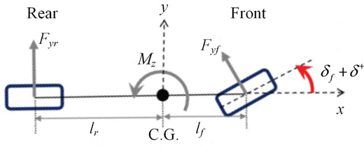
Symbols of vehicle model

Symbol	Description
R	Vehicle’s yaw rate
M	The mass of vehicle
δ_f	Front steering angle from driver
δ⁺	External front steering angle from controller
$\overset{\land}{α_{i}}$	Slip angle of tires on axle i with zero steering angle
C_ai	Cornering stiffness of axle i
$\overset{\land}{C_{α i}}$	Estimated cornering stiffness value of axle i by controller
M_z	Yaw moment of tire longitudinal force
R_e	Effective wheel radius of vehicle
D_f, D_r	Front or rear track width
I_z	Yaw moment of vehicle
α_f,α_r	Tire side slip angle at front or rear tire
l_f, l_r	Distance from the center of gravity to front or rear axle
F_yf, F_rr	Lateral force of front or rear tires

Symbol	Description
R	Vehicle’s yaw rate
M	The mass of vehicle
δ_f	Front steering angle from driver
δ⁺	External front steering angle from controller
$\overset{\land}{α_{i}}$	Slip angle of tires on axle i with zero steering angle
C_ai	Cornering stiffness of axle i
$\overset{\land}{C_{α i}}$	Estimated cornering stiffness value of axle i by controller
M_z	Yaw moment of tire longitudinal force
R_e	Effective wheel radius of vehicle
D_f, D_r	Front or rear track width
I_z	Yaw moment of vehicle
α_f,α_r	Tire side slip angle at front or rear tire
l_f, l_r	Distance from the center of gravity to front or rear axle
F_yf, F_rr	Lateral force of front or rear tires

The equations for the yaw dynamic of the vehicle can be described as follows:

\dot{r} = \frac{l_{f} F_{y f} - l_{r} F_{y r} + M_{z}}{I_{z}}

(1)

where r is the yaw rate of the vehicle, l_f is the distance of the front wheel axles from the center of gravity (CG), l_r is the distance of the front wheel axles from the CG, M_x is the external yaw moments for the improve the driving stability of the vehicle and I_z is the yaw inertia of vehicle. The lateral force of the front and rear tires of the vehicle can be expressed as follows:

F_{y f} = l_{f} C_{α f} α_{f} \cos δ_{f}

(2)

F_{y r} = l_{r} C_{α r} α_{r}

(3)

where δ_f is the front wheel steering, C_af is the cornering stiffness of the vehicle’s front wheel, C_ar is the cornering stiffness of the vehicle’s rear wheel, α_f is the slip angle of the front wheel and α_r is the slip angle of the rear wheel. The front and rear wheel slip angles of the vehicle can be expressed as follows:

α_{f} = δ_{f} + δ^{+} + \overset{\land}{α_{f}}

(4)

α_{r} = \overset{\land}{α_{r}}

(5)

where α_i is the slip angle of the front (i = f) and rear (i = r) tires at zero steering wheel angle. $\overset{\land}{α_{i}}$ (i = f = r) can be expressed as follows:

{\overset{\land}{α}}_{i} = - \tan^{- 1} \frac{v_{y} + ζ_{i} l_{i} r}{v_{x}}

(6)

where v_y is the y-direction velocity in the body coordinate system, v_x is the x-direction velocity in the body coordinate system, ζ_f = −ζ_r =1. Equation (7) is deduced using equation (6) as follows:

{\overset{\overset{\cdot}{\land}}{α}}_{i} = \frac{\partial \overset{\land}{α_{i}}}{\partial r} | \underset{r_{0}}{} \dot{r} + \frac{\partial \overset{\land}{α_{i}}}{\partial v_{y}} | \underset{v_{y 0}}{} {\dot{v}}_{y} + \frac{\partial \overset{\land}{α_{i}}}{\partial v_{x}} | \underset{v_{x 0}}{} {\dot{v}}_{x}

(7)

The last term in (7) is negligible as $v_{x}^{2}$ appears in the denominator of its partial derivative. And it is smaller than other two partial derivatives. Therefore, the time derivatives of $\overset{\land}{α}$ can be approximated as follows:

\overset{\overset{\cdot}{\land}}{α} = k_{i, v_{y}} {\dot{v}}_{y} + k_{i, r} \dot{r}

(8a)

k_{i, v_{y}} = \frac{1}{v_{x 0} + {(v_{y 0} + ζ_{i} l_{i} r_{0})}^{2} / v_{x 0}}

(8b)

k_{i, r} = \frac{- ζ_{i} l_{i}}{v_{x 0} + {(v_{y 0} + ζ_{i} l_{i} r_{0})}^{2} / v_{x 0}}

(8c)

The yaw moments M_z in equation (1) can be given as follows:

M_{z} = \frac{D_{f}}{2 R_{e}} \cos δ_{f} (T_{f r} - T_{f l}) - \frac{D_{r}}{2 R_{e}} (T_{r r} - T_{r l}) + \frac{l_{f}}{R_{e}} \sin δ_{f} (T_{f r} + T_{f l})

(9)

where T_ij is the total torque on the wheel ij (ij = fl, fr, rl, rr) and R_e is the effective radius of the tire rolling. The differential equations for the lateral velocity of the vehicle can be expressed as follows:

a_{y} = \frac{1}{m} (C_{α f} α_{f} \cos δ_{f} + C_{α r} α_{r})

(10)

The cornering stiffness of vehicle tires will increase with the increasing vertical load of the vehicle and decrease with the increasing tire slip angle. Therefore, the model accuracy is greatly reduced owing to the transfer of the vertical load and the large change of tire slip angles under different working conditions. The lateral acceleration and yaw velocity of the vehicle can be measured using inertial sensors in the practical application. The actual cornering stiffness of tires is estimated on-line based on the 2DOF dynamic equations of vehicle lateral motion and yaw motion. The specific expressions are as follows:

a_{y 0} = \frac{1}{m} (\overset{\land}{C_{α f}} α_{f 0} \cos δ_{f 0} + \overset{\land}{C_{α r}} α_{r 0})

(11)

I_{z} {\dot{r}}_{0} = l_{f} \overset{\land}{C_{α f}} α_{f 0} \cos δ_{f 0} - l_{r} \overset{\land}{C_{α r}} α_{r 0} + M_{z 0}

(12)

where a_y₀ and ${\dot{r}}_{0}$ are the vehicle lateral acceleration and yaw rate acceleration which acquired at the current sample time, respectively. α_f₀ and α_r₀ are the front wheel slip angle and rear wheel slip angle at current sample time, respectively. M_z₀ is the external yaw moments at current sample time. The cornering stiffness equations of the tires according to equations (11) and (12) are described as follows:

\overset{\land}{C_{α f}} = \frac{I_{z} \dot{r} + m a_{y 0} l_{r} - M_{z 0}}{α_{f 0} (l_{f} + l_{r}) \cos δ_{f 0}}

(13)

\overset{\land}{C_{α r}} = \frac{- I_{z} \dot{r} + m a_{y 0} l_{f} + M_{z 0}}{α_{r 0} (l_{f} + l_{r})}

(14)

where m is the mass of the vehicle and δ_f₀ is the front steering angle at current sample time. The state-space equation can be deduced according to equations (1)–(11) as follows:

{\begin{cases} \dot{x} = A_{c} x+ B_{c} u+ B_{c}^{w} w \\ y = Cx \end{cases}

(15)

where

A_{c} = [\begin{matrix} 0 & 0 & \frac{1}{I_{z}} l_{f} C_{α f} \cos δ_{f} & - \frac{1}{I_{z}} l_{r} C_{α r} \\ - v_{x} & 0 & \frac{1}{m} C_{α f} \cos δ_{f} & \frac{1}{m} C_{α r} \\ 0 & 0 & 0 & 0 \\ 0 & 0 & 0 & 0 \end{matrix}], B_{c} = {[\begin{matrix} \frac{l_{f}}{I_{z} R_{e}} \sin δ_{f} - \frac{D_{f}}{2 I_{z} R_{e}} \cos δ_{f} & 0 & 0 & 0 \\ \frac{l_{f}}{I_{z} R_{e}} \sin δ_{f} + \frac{D_{f}}{2 I_{z} R_{e}} \cos δ_{f} & 0 & 0 & 0 \\ \frac{D_{r}}{2 I_{z} R_{e} k} & 0 & 0 & 0 \\ - \frac{D_{r}}{2 I_{z} R_{e}} & 0 & 0 & 0 \\ \frac{l_{f} C_{α f} \cos δ_{f}}{I_{z}} & \frac{1}{m} C_{α f} \cos δ_{f} & 0 & 0 \\ 0 & 0 & 0 & 0 \end{matrix}]}^{T}

A_{c} = [\begin{matrix} 0 & 0 & \frac{1}{I_{z}} l_{f} C_{α f} \cos δ_{f} & - \frac{1}{I_{z}} l_{r} C_{α r} \\ - v_{x} & 0 & \frac{1}{m} C_{α f} \cos δ_{f} & \frac{1}{m} C_{α r} \\ 0 & 0 & 0 & 0 \\ 0 & 0 & 0 & 0 \end{matrix}], B_{c} = {[\begin{matrix} \frac{l_{f}}{I_{z} R_{e}} \sin δ_{f} - \frac{D_{f}}{2 I_{z} R_{e}} \cos δ_{f} & 0 & 0 & 0 \\ \frac{l_{f}}{I_{z} R_{e}} \sin δ_{f} + \frac{D_{f}}{2 I_{z} R_{e}} \cos δ_{f} & 0 & 0 & 0 \\ \frac{D_{r}}{2 I_{z} R_{e} k} & 0 & 0 & 0 \\ - \frac{D_{r}}{2 I_{z} R_{e}} & 0 & 0 & 0 \\ \frac{l_{f} C_{α f} \cos δ_{f}}{I_{z}} & \frac{1}{m} C_{α f} \cos δ_{f} & 0 & 0 \\ 0 & 0 & 0 & 0 \end{matrix}]}^{T}

where u is the control input variable, $T_{f l}^{a d d} and T_{f r}^{a d d}$ are the external driving motor torque of the left and right on the front axle, respectively. $T_{r l}^{a d d} and T_{r r}^{a d d}$ are the external driving motor torque of the left and right on the rear axle, respectively. δ⁺ is the external front steering angle, ϵ is the slack variable associated with the soft constraint on the lateral velocity, w = δ_f is the driver’s steering wheel input which can be regarded as an external disturbance, C is the output matrix, y = v_y is the output variable of the predictive model, A_c, B_c and $B_{c}^{w}$ are the state matrix of the state-space equation which is updated in each control cycle. The discrete-time expressions are computed using the forward Euler discretization method as follows:

A_{c d} = A_{c} T_{s} + I

(16)

B_{c d} = B_{c} T_{s}

(17)

B_{c d}^{w} = B_{c}^{w} T_{s}

(18)

where T_s is the sample period and I is the unit matrix.

3. Controller design

The controller is designed based on MPC algorithm in this section. Firstly, the physical restrictions of the actuator are considered as the controller input constraint. A soft constraint on vehicle lateral velocity is designed for the controller output constraint. The objective function is designed and converted to the quadratic programming form to solve the optimal solution.

3.1 Constraints and objective function

To improve the safety and stability performance of the vehicle in high speed, the lateral velocity is controlled in a certain range by restricting the lateral velocity of the vehicle. The sideslip of the vehicle can be controlled in the stable range. The specific lateral velocity constraint equation is as follows:

| y_{k} | \leq v_{x 0} \tan β_{\max} + ε_{k}

(19)

where β_max > 0 is the maximum allowable sideslip angle value, ε_k > 0 is the slack variable, and it is generated by the controller. To ensure the actuator can respond to the commands that the controller generated in real time, the values of steering angle and the external driving motor torque should be constrained. The specific expression can be described as follows:

{\begin{cases} T_{\min}^{a d d} \leq T_{i j} \leq T_{\max}^{a d d} \\ δ_{\min}^{a d d} \leq δ^{+} \leq δ_{\max}^{a d d} \\ 0 \leq ε_{k} \leq + \infty \end{cases}

(20)

Based on equation (20), it can be rewritten as follows:

lb \leq u \leq ub

(21)

where

lb = {[\begin{matrix} T_{\min}^{a d d} & δ_{\min}^{+} & 0 \end{matrix}]}^{T}, ub = {[\begin{matrix} T_{\max}^{a d d} & δ_{\max}^{+} & \infty \end{matrix}]}^{T}

where T_ij are represent the external driving motor torque of the four wheel, $T_{\min}^{a d d}$ and $T_{\max}^{a d d}$ are represent the minimum and maximum values of the external driving motor torque, respectively; $δ_{\min}^{a d d}$ and $δ_{\min}^{a d d}$ represent the minimum and maximum values of the external steering angle, respectively. The objective function is designed as follows:

J = \frac{1}{2} \sum_{K = 1}^{N_{P}} ({‖ u_{k} - v ‖}_{R}^{2} + {‖ u_{k} - u_{p} ‖}_{T}^{2} +2 z^{T} u_{k})

(22)

where

u_{k} = {[T_{f l}^{a d d} T_{f r}^{a d d} T_{r l}^{a d d} T_{r r}^{a d d} δ^{+} ε]}^{T} v = {[T_{f l}^{d r v} T_{f r}^{d r v} T_{r l}^{d r v} T_{r r}^{d r v} 0 0]}^{T}, z = {[0 0 0 0 0 r_{1 ε}]}^{T},

R = diag {[r_{T} r_{T} r_{T} r_{T} r_{δ} r_{2 ε}]}^{T}, T = diag {[t_{T} t_{T} t_{T} t_{T} t_{δ} t_{ε}]}^{T},

where N_p represents the predictive time domain. $T_{f l}^{d r v}$ and $T_{f r}^{d r v}$ represent the driver input torque of the left and right on the front axle, respectively; $T_{r l}^{d r v} and T_{r r}^{d r v}$ represent the driver input torque of the left and right on the rear axle, respectively; u_k is the desired variable generated by the controller, u_p is the previous desired variable generated by the controller, r_T and r_δ denote the weights of the external torque and external steering angle, respectively; r₁_ε and r₂_ε denote the weights of the corresponding slack factor, T is the positive definite matrix. The first term of the objective function is to produce external control quantities when the controller detects the vehicle in dangerous driving state. There is no external control quantity produced when the vehicle is under a safe driving state. The second term of the objective function is to produce smooth control quantity and to avoid the oscillation. The third term of the objective function is to prevent the solution in failure.

3.2 Quadratic programming setup

To solve the optimal quantities conveniently, the objective function is transformed into quadratic programming. In the prediction time domain N_p, the output vector $\bar{y}$ of the discrete state prediction model equation can be expressed as follows:

\bar{y} = S_{x} x_{0} + S_{u} \bar{u} + S_{w} \bar{w}

(23)

where

{\bar{y}}^{T} = [\begin{matrix} y_{1}^{T} & y_{2}^{T} & \begin{matrix} \dots & y_{N_{p}}^{T} \end{matrix} \end{matrix}], S_{x}^{T} = [\begin{matrix} {(C A_{c d})}^{T} & {(C A_{c d}^{2})}^{T} & \dots & {(C A_{c d}^{N_{p}})}^{T} \end{matrix}]

S_{u} = [\begin{matrix} C B_{c d} & 0 & \dots & \dots & 0 \\ C A_{c d} B_{c d} & C B_{c d} & 0 & \dots & 0 \\ ⋮ & ⋱ & ⋱ & ⋱ & ⋮ \\ ⋮ & ⋱ & ⋱ & ⋱ & ⋮ \\ C A_{c d}^{^{N_{p} - 1}} B_{c d} & \dots & \dots & \dots & C B_{c d} \end{matrix}], S_{w} = [\begin{matrix} C B_{c d}^{w} & 0 & \dots & \dots & 0 \\ C A_{c d} B_{c d}^{w} & C B_{c d}^{w} & 0 & \dots & 0 \\ ⋮ & ⋱ & ⋱ & ⋱ & ⋮ \\ ⋮ & ⋱ & ⋱ & ⋱ & ⋮ \\ C A_{c d}^{^{N_{p} - 1}} B_{c d}^{w} & \dots & \dots & \dots & C B_{c d}^{w} \end{matrix}]

A standard QP form is expressed in equation (24) based on equation (22):

J = \frac{1}{2} {\bar{u}}^{T} (\bar{R} + \bar{T}) \bar{u} + � \bar{z} - \bar{v} \bar{R} - {\bar{u}}_{p}^{T} \bar{T} �^{T} \bar{u} +constant

(24)

where the constant term can be ignored. The remaining can be described as follows:

\bar{R} = blockdiag \underset{N_{p}}{\underset{︸}{(R, R \dots, R)}}, \bar{T} = blockdiag \underset{N_{p}}{\underset{︸}{(R, R \dots, R)}},

{\bar{u}}^{T} = [u_{1}^{T} u_{2}^{T} u_{3}^{T} \dots u_{N_{p}}^{T}], {\bar{u}}_{p} = [u_{p, 1}^{T} u_{p, 2}^{T} u_{p, 3}^{T} \dots u_{p, N_{p}}^{T}]

\bar{z} = \underset{N_{P}}{\underset{︸}{[z^{T} z^{T} z^{T} \dots z^{T}]}}, \bar{v} = \underset{N_{P}}{\underset{︸}{[v^{T} v^{T} v^{T} \dots v^{T}]}} .

The constraints expression of the controller can be expressed as follows:

{\begin{cases} LB < \bar{u} < UB \\ A_{u} \bar{u} < U B_{u} \end{cases}

(25)

where

L B^{T} = \underset{N_{P}}{\underset{︸}{[l b^{T} l b^{T} \dots l b^{T}]}}, U B^{T} = \underset{N_{P}}{\underset{︸}{[u b^{T} u b^{T} \dots u b^{T}]}}, A_{u} = [\begin{matrix} - \bar{b} + S_{u} \\ - \bar{b} - S_{u} \end{matrix}], U B_{u} = [\begin{matrix} - S_{x} x_{0} - S_{w} \bar{w} + {\bar{V}}_{y} \\ S_{x} x_{0} + S_{w} \bar{w} + {\bar{V}}_{y} \end{matrix}]

where

{\bar{b}}^{T} = {[\begin{matrix} b & 0 & \dots & 0 \\ 0 & b & \dots & 0 \\ ⋮ & ⋱ & ⋱ & 0 \\ 0 & 0 & \dots & b \end{matrix}]}_{N_{p} x 6 N_{p}}, b = [\begin{matrix} 0 & 0 & 0 & 0 & 0 & 1 \end{matrix}], {\bar{V}}_{y} = \underset{N_{p}}{\underset{︸}{[\begin{matrix} v_{y_{\max}} & v_{y_{\max}} & \dots & v_{y_{\max}} \end{matrix}]}}

To reduce the computation, accelerate the computation speed and improve the real-time performance, it is assumed that the controlled quantity is invariant when the predictive time domain step exceeds the control time domain N_c:

u_{k} = u_{N_{c}}, N_{c} \leq k \leq N_{p}

(26)

The first vector in the u_k contains the external driving motor torque and front steering angle, which should be transferred to the actuators.

4. Simulation tests

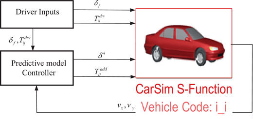
To verify the effectiveness of the proposed method, we adopt the joint simulation platform of Carsim and Matlab/Simulink. The system structure is shown in Figure 2. The stability controller generates the external yaw moments and external front wheel angle when vehicle is under the dangerous condition. The parameters of the vehicle model are shown in Table 2. The parameters of the controller are shown in Table 3. The simulations are performed under various driving scenarios and road conditions. The proposed controller is named MPC, which performance is compared with a proportion & integral (PI) controller and without control. In addition, to further show the advantage of the proposed method, a linear quadratic regulator (LQR) method is also adopted in the simulation.

Figure 2

View large Download slide

Control system architecture

Table 2

Vehicle model parameters

Parameter	Description	Value	Unit
M	Vehicle’s mass	1650	[kg]
I_z	Vehicle’s yaw inertia	3234	[kg m²]
*l_f*	Distance from C.G. to the center of front axle	1.4	[m]
*l_r*	Distance from C.G. to the center of rear axle	1.650	[m]
*h_CG*	Height of C.G	0.53	[m]
*D_f*	Front trackwidth	1.58	[m]
*D_r*	Rear trackwidth	1.58	[m]
*R_e*	Wheel’s effective radius	0.32	[m]

Parameter	Description	Value	Unit
M	Vehicle’s mass	1650	[kg]
I_z	Vehicle’s yaw inertia	3234	[kg m²]
*l_f*	Distance from C.G. to the center of front axle	1.4	[m]
*l_r*	Distance from C.G. to the center of rear axle	1.650	[m]
*h_CG*	Height of C.G	0.53	[m]
*D_f*	Front trackwidth	1.58	[m]
*D_r*	Rear trackwidth	1.58	[m]
*R_e*	Wheel’s effective radius	0.32	[m]

Table 3

Controller parameters

Parameter	Description	Value
*T_s*	Controller sample time (s)	0.02
*N_p*	Size of the prediction horizon	12
*N_c*	Size of the control horizon	3
β_max	Allowable vehicle sideslip angle (deg)	3
*r_T*	Quad. weight of torque adjustments	1 × 10⁻⁷
r₂_ε	Quad. weight of slack variable	0.7
r₁_ε	Linear weight of slack variable	0.045
*t_T*	Quad. weight of torque change	1 × 10⁻⁵
$T_{\max}^{a d d}$	Maximum external driving motor torque (N m)	1,000
$T_{\min}^{a d d}$	Minimum external driving motor torque (N m)	−1,000
$δ_{\max}^{+}$	Maximum front wheel steering adjustment(deg)	10
$δ_{\min}^{+}$	Minimum front wheel steering adjustment(deg)	−10

Parameter	Description	Value
*T_s*	Controller sample time (s)	0.02
*N_p*	Size of the prediction horizon	12
*N_c*	Size of the control horizon	3
β_max	Allowable vehicle sideslip angle (deg)	3
*r_T*	Quad. weight of torque adjustments	1 × 10⁻⁷
r₂_ε	Quad. weight of slack variable	0.7
r₁_ε	Linear weight of slack variable	0.045
*t_T*	Quad. weight of torque change	1 × 10⁻⁵
$T_{\max}^{a d d}$	Maximum external driving motor torque (N m)	1,000
$T_{\min}^{a d d}$	Minimum external driving motor torque (N m)	−1,000
$δ_{\max}^{+}$	Maximum front wheel steering adjustment(deg)	10
$δ_{\min}^{+}$	Minimum front wheel steering adjustment(deg)	−10

4.1 Simulation 1

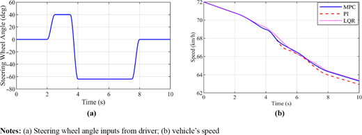
In this simulation, the vehicle is performed under critical working conditions on the ice road with friction coefficient µ = 0.3. Figure 3 shows the input of the steering wheel and the vehicle speed. The driving scenario is a sharp turning maneuver at an initial speed 72 km/h, with steering to the left and hold a few seconds, then quickly counter-steering to the right and finally returning to zero. All maneuvers are performed without applying any acceleration or brake. With these maneuvers the vehicle is usually prone to drift under low friction coefficient road. The longitudinal speed is shown in Figure 3(b).

Figure 3

View large Download slide

Simulation results on the ice road with friction coefficient with μ = 0.3

The vehicle’s sideslip angle and yaw rate are given in Figure 4. Without any controller, it is easy to see the sideslip angle, and the yaw rate of the vehicle increases monotonically when the steering angle returns to zero at t > 4, which indicates the loss of stability of vehicle. In Figure 4(a), the vehicle sideslip angle is well regulated by the proposed MPC controller. Compared to the proposed controller, the sideslip angles by the LQR and PI controller are larger, and the oscillation times are longer. In Figure 4(b), the yaw rate is also regulated by the proposed controller. Without any control, the vehicle is side slipping. PI controller is useful in regulating the vehicle but has larger oscillation. The LQR controller has better performance than PI, but the oscillation is large at 8 s, which is worse compared with the proposed MPC controller.

Figure 4

View large Download slide

Simulation results on the ice road with friction coefficient of μ = 0.3

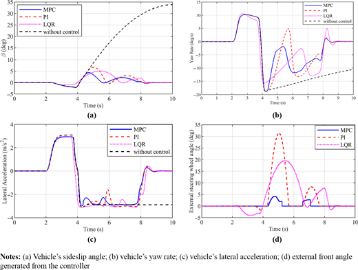
Note that the maximum lateral acceleration is close to 0.3 g in Figure 4(c), which is near the road-tire friction limits at about t > 4 s. In such conditions, the vehicle without controller is drifting and losing stability. The PI controller can stop the phenomenon; however, the oscillation time is longer and control performance is poor, compared with the proposed controller. The proposed MPC controller can still regulate the vehicle and prevent side slipping, which is helpful for the driver to handle the vehicle. The LQR controller has similar performance with the proposed controller. The external front angle generated from the controller is shown in Figure 4(d). From the figure we can see that the external front angle generated from the MPC controller is smaller than PI controller and LQR controller. This means the vehicle can be regulated with smaller steering intervention, which is better for the driver handling the vehicle.

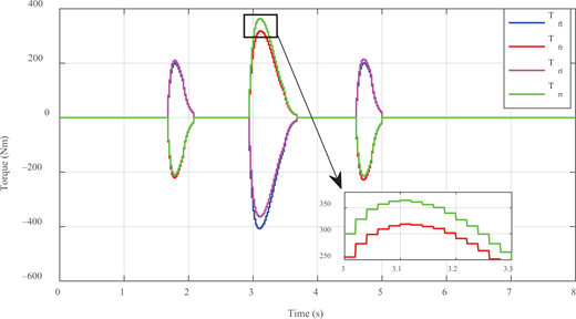
The external driving motor torque from the proposed MPC controller is given in Figure 5. Note that the sideslip controller is activated only when the sideslip angle is larger than 3°. From the figure, it can be seen that controller generates the corresponding control signals to reduce the vehicle’s sideslip, when the vehicle’s sideslip angle is detected to be greater than the safety threshold.

Figure 5

View large Download slide

External driving motor torque the from MPC controller on the ice road with friction coefficient of μ = 0.3

The main advantages of the FWID-EV are the independent driving torque control of the four wheels. Thus, we balance the weight on the front wheel angle and the weight on driving torque. In Figure 5, when the vehicle sideslip angle is close to the value of the threshold at about t > 4.4 s, the controller generates the external driving motor torque with similar size and opposite direction on both sides of the vehicle. This produces the external yaw moments, which reduces the absolute value of the vehicle’s sideslip angle and ensure the vehicle in safety state.

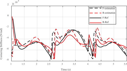
Finally, the tire cornering stiffness estimation results are given in Figure 6. From the figure, the estimated value of the tire cornering stiffness is close to the real value, which also proves the effective of the proposed controller.

Figure 6

View large Download slide

Simulation results of tire cornering stiffness estimation on the ice road with friction coefficient of μ = 0.3. F-estimation: front wheel estimation; R-Real: rear wheel estimation; F-Ref: front wheel reference; R-Ref: rear wheel reference

4.2 Simulation 2

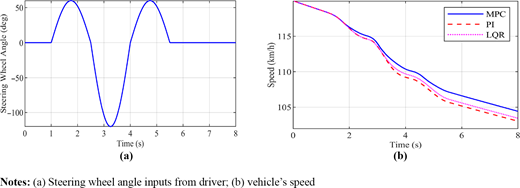
To test the controller under other conditions, a test with high friction coefficient and relatively higher speed is performed. The tire-road friction coefficient is 0.8. The initial speed of the vehicle is 120 km/h.

The driver input of the steering wheel and the vehicle speed are shown in Figure 7(a) and (b), respectively. The driving scenario is a double lane change maneuver at an initial speed 120 km/h, with steering to the left and hold a few seconds, then quickly counter-steering to the right, and then to the left, finally returning to zero. All maneuvers are performed without applying any acceleration or brake. With these maneuvers the vehicle are usually prone to drift under high speed.

Figure 7

View large Download slide

Simulation results on the road with friction coefficient with μ = 0.8

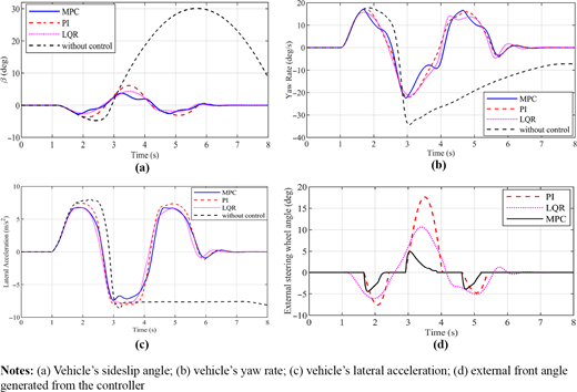
The vehicle’s sideslip angle and yaw rate are shown in Figure 8(a) and (b), respectively. It can be seen that the vehicle’s sideslip angle starts to exceed the threshold value at about 1.6 s. After 0.5 s, the vehicle’s sideslip angle decreases into the threshold range. At about 2.9 s, the sideslip angle increases quickly and exceeds the threshold. The controller is activated and the corresponding control signals are generated to regulate the vehicle. In Figure 8(a), the vehicle is out of control at the very sharp maneuver without control. The PI controller can stabilize the vehicle with larger overshot and longer oscillation than LQR and MPC controller. The LQR controller can regulate the vehicle; however, the steering intervention is larger than that of MPC controller. The external front angle and external driving motor torque generated from the controller are shown in Figures 8(d) and 9, respectively. Compared with PI and LQR controller, the proposed controller can regulate the vehicle well, with relatively smaller steering intervention, which can be used to enhance the advantages of the FWID-EV.

Figure 8

View large Download slide

Simulation results on the road with friction coefficient of μ = 0.8

Figure 9

View large Download slide

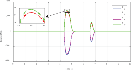
External driving motor torque the from MPC controller on the road with friction coefficient of μ = 0.8

Note that in Figure 8(c) the maximum lateral acceleration is close to 0.8 g, which is close to the limit of the tire-road friction. In such conditions, the vehicle without controller is drifting and unstable. The PI and LQR controller can stop the phenomenon; however, steering intervention is larger compared with the proposed controller. The smaller steering intervention, the better the handling ability. The proposed MPC controller can still regulate the vehicle and prevent side slipping, which is helpful for the driver to handle the vehicle. Figure 9 shows the external driving motor torque generated by the proposed controller. It can be seen that at about 1.6 and 2.9 s, the external driving motor torque is generated as soon as the vehicle sideslip angle exceeds the threshold value. The tire cornering stiffness estimation results are given in Figure 10. From the figure, the estimated value of the tire cornering stiffness is close to the real value, which also proves the effective of the proposed controller.

Figure 10

View large Download slide

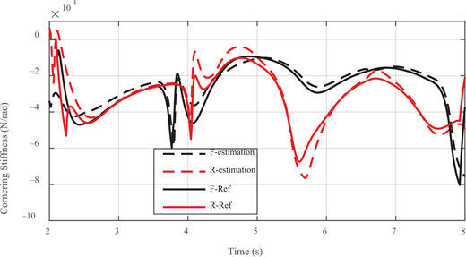
Simulation results of tire cornering stiffness estimation on the road with friction coefficient of μ = 0.8. F-estimation: front wheel estimation; R-Real: rear wheel estimation; F-Ref: front wheel reference; R-Ref: rear wheel reference

5. Conclusion

To enhance the handling and stability of intelligent EVs, this paper adopts a novel MPC algorithm to regulate the vehicle lateral dynamics. The main works of the paper are as follows.

First, based on the bicycle model, we establish the MPC schema and design the objective function. The integrated AFS/DYC strategy is simultaneously adopted in the model.

Second, to control the lateral dynamics, the vehicle’s sideslip angle is chosen as the constraint and is controlled in stable range. When the vehicle’s sideslip angle is in the stable range, the proposed controller is not activated. On the contrary, when the vehicle’s sideslip angle reaches the dangerous values, the proposed method quickly generates the external front steering angle and external driving motor torque to regulate the vehicle lateral dynamics.

Third, the online estimation of tire stiffness is performed. Considering the tire lateral stiffness varied with the different working condition, we choose the vehicle’s lateral acceleration and the yaw rate acceleration into the 2DOF equation to solve the tire cornering stiffness in real time. This can ensure the accuracy of model.

Finally, we perform simulation tests to verify the proposed MPC controller on the Matlab/Simulink/Carsim joint platform. The results of simulation show that the proposed method can ensure the vehicle handling and stability, especially in dangerous working condition.

This work is partly supported by National Natural Science Foundation of China (51605108) and Natural Science Foundation of Guangxi Province (2020GXNSFAA297031, 2018GXNSFAA281271, Guike2018AD19065).

References

Cao

,

M.

,

Hu

,

C.

,

Wang

,

J.

,

Wang

,

R.

and

Chen

,

N.

(

2020

), “

Adaptive complementary filter-based post-impact control for independently-actuated and differentially-steered autonomous vehicles

”,

Mechanical Systems and Signal Processing

, Vol.

144

, p.

106852

, doi:

https://doi.org/10.1016/j.ymssp.2020.106852

.

Google Scholar

Crossref

Geng

,

C.

,

Mostefai

,

L.

,

Denai

,

M.

and

Hori

,

Y.

(

2009

), “

Direct yaw-moment control of an in-wheel-motored electric vehicle based on body slip angle fuzzy observer

”,

IEEE Transactions on Industrial Electronics

, Vol.

56

, pp.

1411

-

1419

.

Google Scholar

Crossref

Guo

,

J.

,

Luo

,

Y.

and

Li

,

K.

(

2019

), “

Robust gain-scheduling automatic steering control of unmanned ground vehicles under velocity-varying motion

”,

Vehicle System Dynamics

, Vol.

57

No.

4

, pp.

595

-

616

.

Google Scholar

Crossref

Guo

,

J.

,

Luo

,

Y.

,

Li

,

K.

and

Dai

,

Y.

(

2018

), “

Coordinated path-following and direct yaw-moment control of autonomous electric vehicles with sideslip angle estimation

”,

Mechanical Systems and Signal Processing

, Vol.

105

, pp.

183

-

199

.

Google Scholar

Crossref

Hori

,

Y.

(

2014

), “

Future vehicle driven by electricity and control - Research on four-wheel-motored UOT electric march II

”,

IEEE Transactions on Industrial Electronics

, Vol.

51

No.

5

, pp.

954

-

962

.

Google Scholar

Crossref

Jalali

,

M.

,

Hashemi

,

E.

,

Khajepour

,

A.

,

Chen

,

S.

and

Litkouhi

,

B.

(

2018

), “

A combined-slip predictive control of vehicle stability with experimental verification

”,

Vehicle System Dynamics

, Vol.

56

No.

2

, pp.

319

-

340

.

Google Scholar

Crossref

Jiang

,

K.

,

Zhang

,

H.

,

Karimi

,

H.

,

Lin

,

J.

and

Song

,

L.

(

2020

), “

Simultaneous input and state estimation for integrated motor-transmission systems in a controller area network environment via an adaptive unscented Kalman filter

”,

IEEE Transactions on Systems, Man, and Cybernetics: Systems

, Vol.

50

No.

4

, pp.

1570

-

1579

.

Google Scholar

Crossref

Lin

,

F.

,

Zhang

,

Y.

,

Zhao

,

Y.

,

Yin

,

G.

,

Zhang

,

H.

and

Wang

,

K.

(

2019

), “

Trajectory tracking of autonomous vehicle with the fusion of DYC and longitudinal-lateral control

”,

Chinese Journal of Mechanical Engineering

, Vol.

32

No.

1

, doi:

https://doi.org/10.1186/s10033-019-0327-9

.

Google Scholar

Liu

,

Y.

,

Wang

,

J.

,

Chen

,

C.

,

Xu

,

Q.

and

Li

,

L.

(

2020

), “

Vehicle safety analysis at non-signalised intersections at different penetration rates of collision warning systems

”,

IET Intelligent Transport Systems

, Vol.

14

No.

13

, pp.

1759

-

1768

, doi:

https://doi.org/10.1049/iet-its.2019.0505

.

Google Scholar

Crossref

Lyckegaard

,

A.

,

Hels

,

T.

and

Bernhoft

,

I.

(

2015

), “

Effectiveness of electronic stability control on single-vehicle accidents

”,

Traffic Injury Prevention

, Vol.

16

No.

4

, pp.

380

-

386

.

Google Scholar

Crossref

PubMed

Mangia

,

A.

,

Lenzo

,

B.

and

Sabbioni

,

E.

(

2021

), “

An integrated torque-vectoring control framework for electric vehicles featuring multiple handling and energy efficiency modes selectable by the driver

”,

Meccanica

, Vol.

56

No.

5

, pp.

991

-

1010

, doi:

https://doi.org/10.1007/s11012-021-01317-3

.

Google Scholar

Crossref

Nam

,

K.

,

Oh

,

S.

,

Fujimoto

,

H.

and

Hori

,

Y.

(

2012

), “

Robust yaw stability control for electric vehicles based on active front steering control through a steer-by-wire system

”,

International Journal of Automotive Technology

, Vol.

13

No.

7

, pp.

1169

-

1176

.

Google Scholar

Crossref

Ni

,

J.

,

Hu

,

J.

and

Xiang

,

C.

(

2017

), “

Envelope control for four-wheel independently actuated autonomous ground vehicle through AFS/DYC integrated control

”,

IEEE Transactions on Vehicular Technology

, Vol.

66

No.

11

, pp.

9712

-

9726

.

Google Scholar

Crossref

Ni

,

J.

,

Wang

,

W.

,

Hu

,

J.

and

Xiang

,

C.

(

2019

), “

Relaxed static stability for four-wheel independently actuated ground vehicle

”,

Mechanical Systems and Signal Processing

, Vol.

127

, pp.

35

-

49

.

Google Scholar

Crossref

Peng

,

H.

,

Wang

,

W.

,

An

,

Q.

,

Xiang

,

C.

and

Li

,

L.

(

2020

), “

Path tracking and direct yaw moment coordinated control based on robust MPC with the finite time horizon for autonomous independent-drive vehicles

”,

IEEE Transactions on Vehicular Technology

, Vol.

69

No.

6

, pp.

6053

-

6066

, doi:

https://doi.org/10.1109/TVT.2020.2981619

.

Google Scholar

Crossref

Poussot-Vassal

,

C.

,

Sename

,

O.

,

Dugard

,

L.

and

Savaresi

,

S.

(

2011

), “

Vehicle dynamic stability improvements through gain-scheduled steering and braking control

”,

Vehicle System Dynamics

, Vol.

49

No.

10

, pp.

1597

-

1621

.

Google Scholar

Crossref

Ren

,

B.

,

Chen

,

H.

,

Zhao

,

H.

and

Yuan

,

L.

(

2016

), “

MPC-based yaw stability control in in-wheel-motored EV via active front steering and motor torque distribution

”,

Mechatronics

, Vol.

38

, pp.

103

-

114

.

Google Scholar

Crossref

Tjonnas

,

J.

and

Johansen

,

T.

(

2010

), “

Stabilization of automotive vehicles using active steering and adaptive brake control allocation

”,

IEEE Transactions on Control Systems Technology

, Vol.

18

No.

3

, pp.

545

-

558

.

Google Scholar

Crossref

Wang

,

R.

,

Zhang

,

H.

and

Wang

,

J.

(

2014

), “

Linear parameter-varying controller design for four-wheel independently actuated electric ground vehicles with active steering systems

”,

IEEE Transactions on Control Systems Technology

, Vol.

22

, pp.

1281

-

1296

.

Google Scholar

Xiao

,

D.

,

Yuan

,

Q.

,

Kang

,

S.

and

Xu

,

X.

(

2021

), “

Insights on crash injury severity control from novice and experienced drivers: a bivariate random-effects probit analysis

”,

Discrete Dynamics in Nature and Society

, Vol.

2021

, doi:

https://doi.org/10.1155/2021/6675785

.

Google Scholar

Xu

,

Q.

,

Wang

,

J.

,

Wang

,

B.

and

Yan

,

X.

(

2020

), “

Modeling and simulation of intersection quasi-moving block speed guidance based on connected vehicles

”,

Journal of Intelligent and Connected Vehicles

, Vol.

3

No.

2

, pp.

67

-

78

. (

2020

).

Google Scholar

Crossref

Xue

,

W.

,

Zheng

,

R.

,

Yang

,

B.

,

Wang

,

Z.

and

Kaizuka

,

T.

(

2019

), “

An adaptive model predictive approach for automated vehicle control in fallback procedure based on virtual vehicle scheme

”,

Journal of Intelligent and Connected Vehicles

, Vol.

2

No.

2

, pp.

67

-

77

.

Google Scholar

Crossref

Yang

,

X.

,

Wang

,

Z.

and

Peng

,

W.

(

2009

), “

Coordinated control of AFS and DYC for vehicle handling and stability based on optimal guaranteed cost theory

”,

Vehicle System Dynamics

, Vol.

47

No.

1

, pp.

57

-

79

.

Google Scholar

Crossref

Zhang

,

H.

,

Zhang

,

G.

and

Wang

,

J.

(

2016

), “

H-infinity observer design for LPV systems with uncertain measurements on scheduling variables: application to an electric ground vehicle

”,

IEEE/ASME Transactions on Mechatronics

, Vol.

21

No.

3

, pp.

1659

-

1670

.

Google Scholar

Crossref

Zhang

,

W.

,

Wang

,

Z.

,

Drugge

,

L.

and

Nybacka

,

M.

(

2020

), “

Evaluating model predictive path following and yaw stability controllers for over-actuated autonomous electric vehicles

”,

IEEE Transactions on Vehicular Technology

, Vol.

69

No.

11

, pp.

12807

-

12821

.

Google Scholar

Crossref

Zhao

,

W.

and

Zhang

,

H.

(

2018

), “

Coupling control strategy of force and displacement for electric differential power steering system of electric vehicle with motorized wheels

”,

IEEE Transactions on Vehicular Technology

, Vol.

67

No.

9

, pp.

8118

-

8128

.

Google Scholar

Crossref

Zhao

,

W.

,

Qin

,

X.

and

Wang

,

C.

(

2018

), “

Yaw and lateral stability control of automotive four-wheel steer-by-wire system

”,

IEEE/ASME Transactions on Mechatronics

, Vol.

23

No.

6

, pp.

2628

-

2637

.

Google Scholar

Crossref

2021

Cong Li, YunFeng Xie, Gang Wang, XianFeng Zeng and Hui Jing.

Published in Journal of Intelligent and Connected Vehicles. Published by Emerald Publishing Limited. This article is published under the Creative Commons Attribution (CC BY 4.0) licence. Anyone may reproduce, distribute, translate and create derivative works of this article (for both commercial and non-commercial purposes), subject to full attribution to the original publication and authors. The full terms of this licence maybe seen at http://creativecommons.org/licences/by/4.0/legalcode

Lateral stability regulation of intelligent electric vehicle based on model predictive control

1. Introduction

2. System modeling

3. Controller design

3.1 Constraints and objective function

3.2 Quadratic programming setup

4. Simulation tests

4.1 Simulation 1

4.2 Simulation 2

5. Conclusion

References

Email Alerts

Cited By

Lateral stability regulation of intelligent electric vehicle based on model predictive control Open Access

1. Introduction

2. System modeling

3. Controller design

3.1 Constraints and objective function

3.2 Quadratic programming setup

4. Simulation tests

4.1 Simulation 1

4.2 Simulation 2

5. Conclusion

References

Email Alerts

Suggested Reading

Recommended for you

Cited By

Gift article access

Gift article access

Gift article access

Gift article access

Sharing Unavailable

Lateral stability regulation of intelligent electric vehicle based on model predictive control