


The purpose of this paper is to reduce the difficulty of model predictive control (MPC) deployment on FPGA so that researchers can make better use of FPGA technology for academic research.
In this paper, the MPC algorithm is written into FPGA by combining hardware with software. Experiments have verified this method.
This paper implements a ZYNQ-based design method, which could significantly reduce the difficulty of development. The comparison with the CPU solution results proves that FPGA has a significant acceleration effect on the solution of MPC through the method.
Due to the limitation of practical conditions, this paper cannot carry out a hardware-in-the-loop experiment for the time being, instead of an open-loop experiment.
This paper proposes a new design method to deploy the MPC algorithm to the FPGA, reducing the development difficulty of the algorithm implementation on FPGA. It greatly facilitates researchers in the field of autonomous driving to carry out FPGA algorithm hardware acceleration research.
1. Introduction
Compared with other control methods, model predictive control (MPC) has many advantages: low requirements on model accuracy, good robustness and effective handling of multivariate constraint problems (Fernandez-Camacho and Bordons-Alba, 1995). Besides, MPC has succeeded in the field of industrial process control (Yu-Geng et al., 2013). Therefore, in recent years, it has been widely used in the field of autonomous driving (Goli and Eskandarian, 2019; Quan and Chung, 2019; Li et al., 2010). However, MPC often shows low efficiency in solving real-time tasks due to a large amount of calculation (Yu-Geng et al., 2013). Researchers hope that the high-performance computing platform’s computing capacity can make up for this defect of MPC. The core of the hardware computing platform is the processor chip. Currently, mainstream chips include CPU, graphics processing unit (GPU), FPGA and application specific integrated circuit (ASIC). The parallel computing capabilities of GPU, FPGA and ASIC are far superior to CPU. They are often used as hardware accelerators. Among these three chips, FPGA has the absolute advantage in power consumption over GPU and has reversible development characteristics compared with ASIC (Falsafi et al., 2017; Nurvitadhi et al.,2016; Kestur et al., 2010; Qasaimeh et al., 2019; Kuon and Rose, 2007; Jones et al., 2010; Russo et al., 2012). With these characteristics, FPGA is more adaptable to algorithms update, making it widely welcomed by researchers.
How to use FPGA to accelerate MPC is a problematic point. Summarizing the existing studies, the primary way to realize the hardware-accelerated solution of MPC by FPGA is through using hardware description languages. For example, He and Ling (2005) used Handle-C hardware description language to implement the accelerated solution of MPC on FPGA for the first time. Following this, Jerez et al. (2012) described a parameterizable FPGA application architecture, which mainly used a deep pipeline structure; as the solution scale increases, the MPC acceleration effect is gradually significant. Jerez et al. (2014) proposed a sharable hardware architecture based on the fast gradient descent method and the alternating multiplier method to solve the MPC problem, which can save a lot of hardware resources.
However, in the field of autonomous driving, researchers are better at high-level languages. Hardware language is too difficult for them. Benefitted from the development of electronic design automation technology, researchers can directly use high-level languages through high-level synthesis tools (Martin and Smith, 2009) to realize the mapping of algorithms to hardware. In this way, several achievements have been made in research. For example, Xu et al. (2015) successfully converted the C++ form of MPC into hardware language through Altera’s Quartus II and Mentor’s Catapult Synthesis, and deployed it on Altera Stratix III FPGA. Lucia et al. (2017) used the advanced synthesis tools provided by Xilinx to deploy MPC on XC7A200, which further proved the feasibility of bypassing the direct use of hardware languages and indirect deployment of high-level languages on FPGA.
ZYNQ, as a new generation of Xilinx FPGA products, integrates the processing system based on a dual-core Advanced RISC Machine (ARM) Cortex-A9 and the programmable logic composed of an XC7Z020 FPGA. Compared with the independent FPGA, it owns the high-performance computing power of FPGA and the unparalleled resource allocation ability of CPU. The combination of the two allows researchers to process the algorithm more flexibly. At the same time, ZYNQ also has the advantages of low power consumption and low price.
Although the above methods realized the deployment of MPC to FPGA and proved its feasibility, they were not for ZYNQ. We need a convenient and fast algorithm deployment method for the new generation of FPGA hardware.
The main contribution of this paper is to propose a method to deploy the MPC algorithm to FPGA (ZYNQ), which greatly reduces the difficulty of algorithm implementation on the latter. Our research results lay the foundation for the application of ZYNQ in actual vehicle experiments.
The paper is organized as follows. In Section 2, we design a lateral control algorithm for autonomous vehicles. In Section 3, a software and hardware combination method based on ZYNQ is proposed and realized. The control algorithm’s feasibility, the solution performance of the quadratic programming solver and the acceleration effect of FPGA are verified in Section 4. Section 5 concludes this paper.
2. Lateral control algorithm of autonomous vehicles
Generally, vehicle control consists of lateral control and longitudinal control. For convenience, the trajectory tracking scenario in lateral control is discussed in this section, which will serve as the basis for subsequent study in this paper.
2.1 Dynamic model
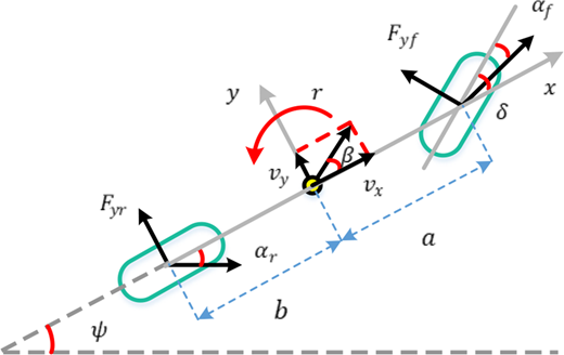
As shown in Figure 1, we choose the single-track bicycle model assuming constant forward speed (Bevly et al., 2006). The vehicle dynamics are described as:
where y is the lateral displacement; vx is the longitudinal speed; Cf is the front wheel cornering stiffness and Cr is the rear wheel cornering stiffness; m is the vehicle mass; a and b are the distances of front and rear axle from the center of gravity; Iz is the moment of inertia; ψ is the yaw angle; β is the vehicle slip angle; r is the yaw rate; δ is the front wheel steering angle.
The state-space equations are obtained as:
where x(k) is the state variable, x(k) = [y ψ β r]T, y(k) is the output variable, y(k) = [y ψ]T, u(k) is the control variable, u(k) = δ,
The discretization form of (2) is:
where A = I + T · Ac, B = T · Bc, C = Cc, T is the sampling time, I is the identity matrix.
For y(k) = C · x(k), we set both the prediction horizon and control horizon to P, then
where
2.2 Cost function and optimization problem
Vehicle lateral control needs to ensure that the autonomous vehicle can track the reference trajectory as close as possible, so in the cost function, we need to consider the deviation between the predicted value of the lateral displacement and the reference value, and the deviation between the predicted value of the yaw angle and the reference value. In summary, the cost function is designed as:
where φ(k + i | k) and φref (k + i | k) are the predicted yaw angle and the reference yaw angle, respectively. and are the predicted lateral displacement and the reference lateral displacement, respectively. u(k + i | k) is the control input, i.e. front-wheel steering angle. q1 denotes the weight coefficient of the yaw angle, while q2 denotes the weight coefficient of the lateral displacement. r is the weight coefficient of the control variable. Y(k + i | k) and Yref (k + i | k) are the predicted values and the reference values. Q is the weight matrix of output variables, and R is the weight matrix of control variables, .
Substituting (4) into (5):
where
Our goal is to minimize (6):
The number of constraints directly determines the dimension of the solution to MPC. To save FPGA hardware resources in the following text, we only restrict the control variable (when hardware resources are sufficient, the performance of FPGA can be extended to MPC with state constraints):
where , umin and umax are the lower and upper limits of the control variable, respectively.
We can rewrite (8) as:
where ,
By combining (7) and (9)
Definition 1: Formula (10) is the standard form of the quadratic programming (QP) problem with constraints. The essence of solving the MPC problem is to solve the QP problem. Each time a set of optimal solution sequence U* is obtained, the first element u* is taken as the control variable.
2.3 Quadratic programming solver
The QP solver used in this paper is Quadprog++ (Di Gaspero, 2007). It is an open-source solver. Compared with other QP solvers such as quadprog, CVXGEN. Quadprog + + has the advantages of simplicity, easy modification and fewer hardware resources occupation (Mattingley and Boyd, 2012; Brandao et al., 2019).
Quadprog++ is written in C++ by Luca Di Gaspero according to the Goldfarb–Idnani method (Goldfarb and Idnani, 1983). The Goldfarb–Idnani method combines the active set algorithm (Nocedal and Wright, 2006) and the dual algorithm to have a fast iteration speed.
Definition 2: The idea of the active set shows that (10) can be transformed into a form of equality constraints:
where S denotes the indices of the active set, N is the active set matrix determined by S, are the elements of B* indexed by S (Horowitz and Afonso, 2002).
According to the KKT conditions (under the transformation x = H1/2 U) (Goldfarb and Idnani, 1983; Horowitz and Afonso, 2002):
where γ* is the Lagrangian multiplier, x* is the optimal solution, and
Cholesky decomposition of H:
Remark 1: The Goldfarb–Idnani method only supports solving positive definite problems (Goldfarb and Idnani, 1983), so H must be a positive definite matrix.
QR decomposition of (K−T N) (Horowitz and Afonso, 2002):
where L is an orthogonal matrix, R is an upper triangular matrix and E contains as many columns as R.
Then N*, M and W can be shown as (Goldfarb and Idnani, 1983):
We set Sk to be the currently active set, Nk, Lk and Rk are the matrixes corresponding to Sk. When Sk is not empty, through Givens rotations, we can get (Horowitz and Afonso, 2002):
According to (12) and (15) (Horowitz and Afonso, 2002):
where xk is the solution and γk is the Lagrangian multiplier corresponding to Sk.
Also, because of the KKT conditions:
where xk+1 is the solution corresponding to Sk ∪ m. n+ is the normal vector of the mth constraint, t is the corresponding Lagrangian multiplier (Horowitz and Afonso, 2002).
According to (15)–(18), the search directions of Goldfarb–Idnani method are defined as (Schmid and Biegler, 1994):
Remark 2: The relevant proof processes of the Goldfarb–Idnani method are shown in literature (Goldfarb and Idnani, 1983).
The pseudo-code of the Goldfarb–Idnani method is shown in the algorithm.
Algorithm Goldfarb-Idnani method (Goldfarb and Idnani, 1983; Horowitz and Afonso, 2002)
Initializing x = −H-1 G = −K-1 K-T G, L = K-1,
S = {∅}, v = 0, v as the cardinality of S
1. if all constrains are satisfied then x is optimal, STOP.
else n+ = np,γ+=[γ 0]T,
if v = 0 then γ+ = 0,
end if;
end if;
S+ = S ∪ {p}, p as the index of constraint to be added to S
2. (a) Search direction in primal space: z = FFT n+
if v > 0 then
search direction in dual space: r = R-1 ET n+
end if;
(b) Step length:
maximum step in dual space: t1
if v = 0 or r ≤ 0 then t1 = ∞
else
end if;
minimum step in primal space: t2
if ‖z‖ = 0 then t2 = ∞
else
end if;
t = min (t1, t2)
(c) if t = ∞ then problem infeasible
end if;
if t2 = ∞, t1 is finite then
S = S\{m}, v = v – 1, update L, R and γ+, go to
2(a)
end if;
set
if , t = t2 then γ = γ+ S = S ∪ {p}, v = v + 1,
update L, R. Go to 1.
else t = t1 then S = S\\{m}, v = v – 1, update L, R, and γ+. Go to 2(a).
end if;
The update operations of the Cholesky, L and R in the Goldfarb–Idnani method account for a large proportion, and they are also the parts that consume the most hardware resources.
3. Implementation quadratic programming solver on FPGA
3.1 Hardware platform selection
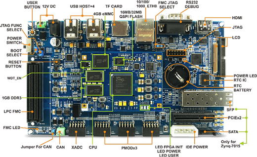
According to our framework, the computation part of the QP solver is fully deployed on the FPGA as it is computing-intensive and time-consuming. The ARM processor is only responsible for data transmission and high-level system control. This kind of scheme can fully use the computing power of FPGA and the flexibility of the ARM processor. In this paper, the MYD-C7Z020 development board (Figure 2) is used as the hardware platform. Table 1 lists the parameters of MYD-C7Z020 and shows its strong ability to adapt to the environment. MYD-C7Z020 is composed of the core board and the bottom board. The core board is embedded with a core function chip such as ZYNQ SoC, while the bottom board is equipped with various functional interfaces, switches and indicators.
3.2 Design flow
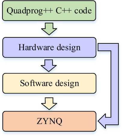
The overall design flow is shown in Figure 3; we follow a software-hardware codesign method to deploy the proposed algorithm. The hardware part is to deploy the QP algorithm to the programmable logic for fast computation and data movement optimization. The software is mainly aimed at the processing system. The purpose is to realize the deployment of the drivers, the data interaction between the on-chip memory and the off-chip interfaces and the self-starting of the hardware development platform.
3.1.1 Hardware design
In hardware design, we first use Xilinx Vivado HLS (Winterstein et al., 2013) to convert the C++ form of the algorithm to register transfer level. We also need to select the functional interface type and the optimization method to implement effective algorithm deployment.
Considering the controller’s control effect and the maximum utilization rate of hardware, we set both the prediction horizon and the control horizon to be five, so the maximum dimension of the matrix calculated on the FPGA is ten. Table 2 shows the hardware resource utilization information of FPGA. FPGA mainly contains four kinds of hardware resources: block random access memory (BRAM), DSP48E, flip flop (FF) and look-up table (LUT). LUT resources are occupied so much because the Goldfarb–Idnani algorithm involves a large number of matrix multiplication and addition operations (the update operations of Cholesky, L and R).
Hardware resources utilization information of FPGA
| BRAM | DSP48E | FF | LUT | |
|---|---|---|---|---|
| Total | 22 | 78 | 30,059 | 47,923 |
| Available | 280 | 220 | 106,400 | 53,200 |
| Utilization | 7% | 35% | 28% | 90% |
The biggest advantage of FPGA is that it uses hardware to perform parallel operations. This type of process is very intuitive, such as a·b + c·d, which can perform a·b and c·d simultaneously. Vivado HLS can perform automatic parallel processing while generating the hardware language. We can also choose to select different optimization methods to process the C++ code manually. According to the specific situation, we select pipeline, unroll and pipeline&unroll. The results are shown in Table 3; neither the resource utilization rate nor the simulation time has been significantly improved (in the follow-up Vivado IDE-related process, these three optimization methods did not pass the verification due to excessive wiring resources). The above results are related to the algorithm structure; if it is composed of a relatively neat neural network structure, these optimization methods will produce significant results.
Comparison of optimization results
| Optimization | Default state | Pipeline | Unroll | Pipeline and unroll |
|---|---|---|---|---|
| BRAM | 22 | 22 | 22 | 22 |
| DSP48E | 78 | 78 | 78 | 78 |
| FF | 30,059 | 30,059 | 30,060 | 30,132 |
| LUT | 47,923 | 47,954 | 48,348 | 48,356 |
| Simulation time | 35,525 ns | 35,445 ns | 35,285 ns | 35,365 ns |
| Delay | 3,534 | 3,526 | 3,510 | 3,518 |
When the above work is completed, we need an environment to achieve corresponding hardware functions, so the algorithm module is imported into the environment generated by Vivado IDE (Crockett et al., 2014). The main contribution of our design is shown in Figure 4. We mainly choose three modules to achieve the corresponding functions (the combination of modules needs to be designed according to the specific functions to be implemented). The advantage of this design is to take up as little additional hardware resources as possible. The entire project’s workflow is that the processing system first writes the matrices H and A*, the vectors G and B* to BRAM and then the IP generated by Vivado HLS reads the data in BRAM and accelerates the solution. When the solution is completed, the processing system reads the result u* from HLS IP (reading and writing data are done in a polling manner). The communication between different modules is realized through the AXI interface.

3.1.2 Software design
The design of the software part is mainly focused on the writing of driver code. The driver makes ARM the core of the entire architecture, and FPGA acts as a hardware accelerator to assist its work. Besides algorithm acceleration, multitasking functions also need to be supported in the development board’s actual application. This situation requires complicated code programming to achieve, which is troublesome for us, so it is necessary to select an embedded system with mature architecture to complete these works. Linux system is the right choice. Popular Linux distributions mainly include Debian, Fedora and Ubuntu. As a newer distribution, Ubuntu inherits all the advantages of the Linux system and has highlights such as easy installation and various auxiliary functions (Al Housani et al., 2009). We choose Ubuntu16.04 as the operating system deployed on the ARM processor.
4. Results
In this section, we mainly verify the effectiveness of the control algorithm, the reliability of the QP solver and the acceleration effect of FPGA through simulation and experiments.
4.1 Verification of lateral control algorithm
We use MATLAB/Simulink and CarSim for cosimulation in the PC to verify the effect of the control algorithm designed in Section 2. Tables 4 and 5 list the main parameters of the vehicle and the parameters of the lateral control algorithm, respectively.
Main parameters of the vehicle
| Vehicle mass | m | 1,420 [kg] |
| Distance of front axle from the center of gravity | a | 1.015 [m] |
| Distance of rear axle from the center of gravity | b | 1.895 [m] |
| Front wheel cornering stiffness | Cf | 72,197 [N/rad] |
| Rear wheel cornering stiffness | Cr | 39,930 [N/rad] |
| Moment of inertia | Iz | 1,536.7 [kg/m2] |
| Longitudinal speed | vx | 20 [km/h] |
Parameters of the lateral control algorithm
| Prediction horizon/Control horizon | P | 5 |
| Sampling time | Ts | 0.02 [s] |
| Output weighting matrix | q | [50 0;0 10] |
| Control weighting coefficient | r | 4 |
| Control variable upper limit | umax | 0.52 [rad] |
| Control variable lower limit | umin | −0.52 [rad] |
Figure 5 shows the simulation results. We choose the double lane-change as the reference trajectory. The maximum error of the lateral displacement between the driving trajectory and the reference trajectory is less than 0.075 m, and the maximum error of the yaw angle is less than 0.098 rad. The above results prove that the lateral control algorithm in Section 2 is effective.
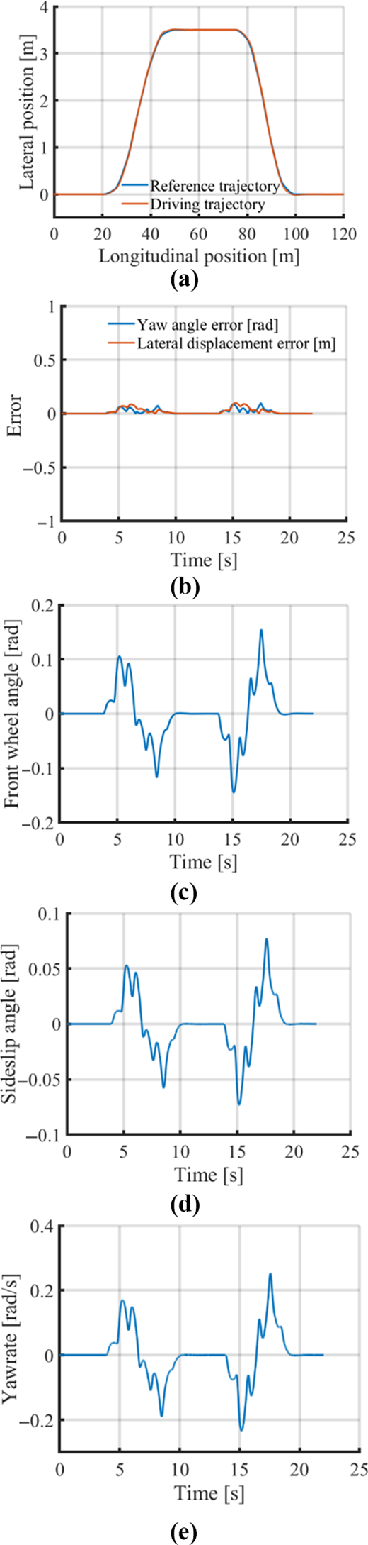
The simulation results. (a) Vehicle trajectory. (b) The error. (c) Front-wheel angle. (d) Sideslip angle. (e) Yaw rate
The simulation results. (a) Vehicle trajectory. (b) The error. (c) Front-wheel angle. (d) Sideslip angle. (e) Yaw rate
4.2 Verification of quadprog++
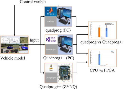
As shown in Figure 6, the performance verification method of Quadprog++ is to ensure the input that is precisely the same as the quadprog solver used in the simulation of part A (Section 4) and then compare the solution accuracy and the solution time of these two solvers. Both solvers run on the PC with the Intel i5 processor at 2.3 GHz. The software platform of quadprog is MATLAB, while Quadprog++’s is Visual Studio.
The comparison results of the solution accuracy are shown in Figure 7. The maximum percentage error of the two solvers is less than 0.008%.
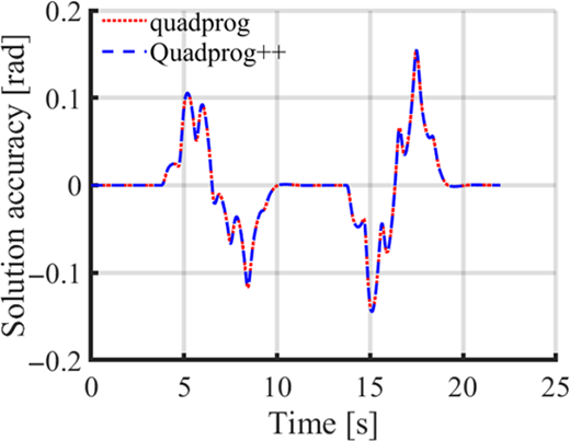
Comparison of the solution accuracy of quadprog and Quadprog++
Comparison of the solution accuracy of quadprog and Quadprog++
Figure 8 and Table 6 present the solution time information of quadrog and Quadprog++. The solution performance of the two solvers is very close.
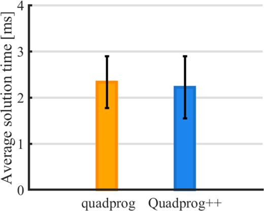
Comparison of the solution time of quadprog and Quadprog++
Comparison of the solution time of quadprog and Quadprog++
Solution time information of QP solvers
| QP Solver | Average solution time | Standard deviation of solution time |
|---|---|---|
| quadprog | 2.332 ms | 0.5645 ms |
| Quadprog++ | 2.216 ms | 0.6723 ms |
The above results prove that Quadprog++ can well meet the solution requirements of the lateral control algorithm in this paper.
4.3 Verification of FPGA
The performance verification method of FPGA (Figure 6) is to use the input that is entirely consistent with the CPU platform and then compare the solution accuracy and the solution time of the two (both use the Quadprog++ solver). The configuration of the CPU is the same as part B (Section 4), and the frequency of ZYNQ is set to 50 MHz.
The comparison results of the solution accuracy are shown in Figure 9. The maximum percentage error of CPU and FPGA is less than 0.04%.
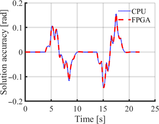
Comparison of the solution accuracy of CPU and FPGA
Comparison of the solution accuracy of CPU and FPGA
As shown in Figure 10 and Table 7, the average solution speed of FPGA is 27.162 times faster than that of CPU and the solution time fluctuation of FPGA is much less than that of the latter.
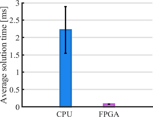
Comparison of the solution time of CPU and FPGA
Comparison of the solution time of CPU and FPGA
Solution time information of hardware platforms
| Hardware platform | Average solution time | Standard deviation of solution time |
|---|---|---|
| CPU | 2.216 ms | 0.6723 ms |
| FPGA | 0.0803 ms | 4.35 × 10⁻⁴ ms |
The above experimental results indicate that compared with CPU, FPGA dramatically improves the speed of solving QP and improves the calculation efficiency of MPC.
5. Conclusion
This paper proposed an FPGA accelerated method of MPC for autonomous driving. Given the difficulty of combining MPC and FPGA. We implement a ZYNQ-based design method, which could significantly reduce the difficulty of development. The comparison with the CPU solution results shows that FPGA has a significant acceleration effect on the solution of MPC (the latter is 27.162 times faster than the former). Our method is effective.
In the future study, we will convert all the floating-point data to fixed-point data to save the hardware resources. We will also carry out relevant actual vehicle experiments to verify the control effect of the selected ZYNQ hardware. At the same time, we will also improve existing algorithms to adapt to more complex scenarios (Keskin et al., 2020).

