

This study investigates the impact of data length on daily demand forecasting accuracy within a horizontal time series structure. While time series data can be structured hierarchically or as forecast intervals, this research focuses on optimizing data length to enhance forecasting performance.
Applying a time series model and the Hidden Markov Model (HMM), this study evaluates daily meal data from a large-scale catering service provider to analyze the impact of different data lengths on forecasting accuracy.
The results indicate that forecasts based on the 3-month data length achieve higher accuracy than those using the 24-month data length. This suggests that utilizing shorter, more recent data segments can enhance forecasting efficiency without compromising accuracy, challenging the traditional assumption that longer historical datasets always yield better predictions.
Forecasting models should align with business strategy and operations. Accurate data collection and validation are essential to prevent forecasting errors. Additionally, regular performance assessment using appropriate accuracy metrics is necessary for refining forecasting models.
This study empirically demonstrates that data length is a key structural factor in forecasting accuracy. Unlike previous research that primarily emphasizes model selection and parameter tuning, this study highlights how optimizing data length improves demand forecasting. By applying these findings to the catering service industry, this study provides actionable insights for businesses seeking to improve operational efficiency through optimized forecasting methodologies.
1. Introduction
One significant factor affecting the accuracy of demand forecasting is the data structures. Time series data, consisting of values collected at regular intervals, is typically organized into two main types: vertical and horizontal. Vertical structures are hierarchical, encompassing levels such as customer, region, or distribution channel. Hierarchical forecasting techniques like Bottom-up, Top-down, and Middle-out are often applied to these levels to enhance forecasting accuracy. In contrast, horizontal structures are defined by forecast intervals such as monthly, weekly, or daily, and are crucial for operational planning, including demand and inventory management. Both vertical and horizontal data structures are essential to accurate forecasting, helping businesses reduce demand uncertainty and improve operational efficiency.
As the volume and length of data rapidly increase across industries, forecasting models are increasingly influenced by these data structures. In service sectors such as last-mile delivery and catering, there is a growing emphasis on real-time operational planning based on short-term forecast intervals (e.g. daily or intra-day). However, generating detailed short-term forecasts for numerous end items (SKUs: Stock Keeping Units) can present significant challenges in terms of time and cost. Traditional demand forecasting methods often rely on long datasets, assuming these datasets capture comprehensive patterns and trends that enhance accuracy. While traditional approaches often rely on longer data lengths for accuracy, this study hypothesizes shorter data lengths can be both efficient and sufficiently accurate for daily demand forecasting by reducing the noise and variability of extended datasets. Data length, in this context, refers to the total duration of time series data used for demand forecasting. For example, it could span 3 months, 1 year, or more, depending on the forecast interval and the requirements of the chosen model.
This research explores the impact of data structure decisions on forecasting accuracy, with a specific focus on determining the optimal data length in a horizontal structure for daily demand forecasting. A theoretical review of existing forecasting methods and data structures is conducted, followed by empirical analysis using daily meal data from a large-scale catering service provider (Company A). The analysis leverages the Hidden Markov Model (HMM) to forecast daily meal demand, highlighting its strength in identifying and predicting patterns in time series data. Notably, shorter datasets facilitate computational efficiency, making complex models like HMM more practical for real-time applications. Additionally, we compare HMM with the widely used Holt-Winters Exponential Smoothing Model (HW), based on previous research (Yoo et al., 2022).
Finally, based on the empirical results, this study proposes an optimal data length for short-term demand forecasting, offering both academic insights and practical implications for improving forecasting accuracy. The research proceeds as follows: Section 2 reviews the theoretical background and relevant prior research, Section 3 outlines the research methodology, including forecasting techniques and evaluation metrics, Section 4 presents the empirical analysis, and Section 5 concludes with the study’s findings and implications.
2. Previous research
2.1 The data structure-based demand forecasting methodology
The hierarchical structure of vertical data has been a significant topic of discussion since the 1950s, focusing on the advantages and limitations of Top-down and Bottom-up approaches. Grunfeld and Griliches (1960), along with Lutkepohl (1984) and Fliedner (1999), argued that Top-down approach can achieve greater accuracy by reducing errors associated with disaggregated data. Conversely, Orcutt et al. (1968) and subsequent studies, including Kinney (1971), Dune et al. (1976), and Gross and Sohl (1990), highlighted Bottom-up approach’s strength in maintaining data integrity during aggregation.
More recent research emphasizes the importance of real demand data and industry-specific characteristics, particularly in multi-level hierarchies. Traditional Top-down approach, which rely on static allocation ratios, may fail to account for temporal changes, leading to less accurate forecasts at lower levels (Athanasopoulos et al., 2009; Mircetic et al., 2017). Alternatively, Middle-out approaches, which focus on intermediate levels such as product families or groups and consider features–functionality, category, and channel–have shown promise in improving forecasting accuracy in complex hierarchical structures (Lo et al., 2008; Yoo et al., 2020).
Horizontal time series data (e.g. monthly, weekly, and daily) is crucial in demand forecasting, helping to analyze volatility factors like seasonality and trends. A minimum of two years (24 months or more) of data is typically required to capture demand fluctuations. In short-term daily demand forecasting, Holt-Winters Exponential Smoothing (HW) and Auto Regressive Integrated Moving Average (ARIMA) are widely used, especially in sectors such as electricity, tourism, and logistics. Taylor (2003) and Weron (2006) demonstrated the effectiveness of ARIMA and bi-seasonal exponential smoothing for electricity demand forecasting. However, Weron (2014) proposed Seasonal ARIMA (SARIMA) to overcome the limitations of ARIMA in modeling trends and improve short-term forecasting accuracy. A summary of recent studies on daily demand forecasting is provided in Table 1.
A literature review on daily demand forecasting using time series models
| Forecasting target | Model | Forecast interval | Data length | Reference |
|---|---|---|---|---|
| Electricity | ARIMA, HW | Daily | 1,460 days | Lee et al. (2013) |
| Food delivery order | SARIMA | Daily | 365 days | Yoon (2016) |
| Electricity | SARIMA | Daily | 1,460 days | Lee and Kim (2019) |
| Air cargo | SARIMA | Daily | 3,217 days | Min and Ha (2020) |
| Port volume | ARIMA | Daily | 2,799 days | Ha et al. (2021) |
Source(s): Yoo et al. (2022)
The required data length for time series models has been widely debated. Box and Jenkins (1976), the developers of the ARIMA model, suggested a minimum of 40–50 past observations to achieve reliable forecasts with narrow forecast intervals. However, various studies have employed different data lengths. For example, Sarpong (2013) used 50 quarterly observations to forecast maternal mortality in Ghana, finding a good fit, while Biswas and Bhattacharyya (2013) applied 57 observations to forecast rice production in West Bengal, with accurate results. In contrast, Alba and Mendoza (2007) used only 24 monthly observations but found this insufficient for capturing key components such as seasonality. Larger datasets, such as those used by Paul et al. (2013) and Al-Masudi (2011), showed that ARIMA models were effective for long-term forecasting. Nowotarski and Weron (2016) also emphasized that data length significantly affects the model’s performance in trend and seasonality estimation. These studies highlight the importance of selecting appropriate data lengths to optimize the performance of time series models.
2.2 The Hidden Markov model (HMM)
The Hidden Markov Model (HMM) is widely recognized for its ability to understand and predict patterns in time series data by considering underlying hidden states. This model has proven highly effective across various domains, including bioinformatics, image processing, speech recognition, and finance (Cappe et al., 2006; Zucchini et al., 2017; Nobakht et al., 2012). A key strength of HMM lies in their ability to model sequential data, recognizing that hidden states govern observable sequences. This feature enables HMM to capture the underlying dynamics of the data, something that traditional time series models, such as exponential smoothing or ARIMA, often fail to do because they do not account for latent factors influencing observed data. Additionally, HMM excels in handling uncertainty by modeling probabilistic transitions between hidden states and the likelihood of observations within those states (Nobakht et al., 2012). This capacity is particularly useful when dealing with noisy or incomplete data, providing a flexible framework for real-time forecasting and dynamic updates as new data is observed. These advantages have made HMM a preferred tool for modeling time-dependent processes in complex environments (Zucchini et al., 2017).
HMM can be defined with three parameters (initial probability: p ,transition probability: A, emission probability: B) to model the relationship between a sequence of states and observations. The components of the Hidden Markov Model (HMM) are presented in Table 2, following the notation provided by Nguyen (2016).
Key components and definitions of the Hidden Markov model (HMM)
| HMM component | Definition |
|---|---|
| Length of observation data | T |
| Number of states | N |
| Number of symbols per state | M |
| Observation sequence | |
| Hidden states sequence | |
| Possible values of each state | |
| Possible symbols per state | |
| Initial probability matrix | |
| Transition probability matrix | |
| Emission probability matrix |
Source(s): Authors’ own work
As shown in Table 2, the parameters required to represent HMM can be defined as . For time series data, a continuous Hidden Markov Model is typically applied by assuming a Gaussian distribution. The three parameters can be expressed as follows:
The primary objective in determining HMM parameters (π, A, B) is to estimate the model parameters that maximize the probability of a given observation sequence. This involves solving three fundamental problems:
How can the probability of a specific observation sequence, given a model, be computed?
Given a model and an observation sequence, what is the most likely sequence of states that generated the observations?
How can the model parameters be estimated using the observed data?
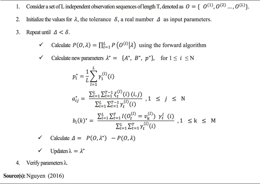
These problems are addressed by the Forward-Backward algorithm, the Viterbi algorithm, and the Baum-Welch algorithm, respectively. Among them, the Baum-Welch algorithm is widely used for parameter estimation in HMM due to its reliable convergence to local maximum likelihood estimates. The algorithm is described as follows:
Baum-Welch algorithm
HMM is widely used in financial markets for predicting exchange rates and stock indices, particularly those with characteristics of continuous time series data, as shown in Table 3.
A literature review on daily demand forecasting using the Hidden Markov model (HMM)
| Forecasting purpose | Forecasting interval | Data length | Reference |
|---|---|---|---|
| Stock price | Daily | 467 days | Hassan and Nath (2005) |
| Stock price | Daily | 401 days | Gupta and Dhingra (2012) |
| Stock price | Daily | 1,520 days | Nguyen (2016) |
| Exchange rate | Daily | 4,030 days | Liu (2018) |
| Stock market | Daily | 2,520 days | Kang and Hwang (2021) |
Source(s): Authors’ own work
2.3 Differentiation from previous research
A review of prior studies on demand forecasting based on data structures reveals that research using vertical data structures frequently employs hierarchical structures and forecasting techniques, while studies on horizontal data structures are increasingly exploring various forecasting intervals. Recent papers, as summarized in Table 1, emphasize the growing interest in daily demand forecasting for practical operational planning. Despite the recognition of the significance of data structure, limited attention has been paid to the effect of data length on forecasting accuracy in existing literature.
This study aims to demonstrate that data length does not need to be extensive and that appropriately adjusting data length can balance forecasting accuracy and efficiency. Specifically, the research focuses on determining the optimal data length for daily demand forecasting. While longer datasets may provide stable trends and seasonality, they often introduce extraneous factors, such as outdated trends, outliers, or irrelevant seasonal fluctuations, which can reduce forecasting accuracy and increase computational demands. In contrast, shorter data lengths minimize noise and better reflect recent patterns, which are critical for accurate short-term forecasting. As seen in Table 1 and Table 3, previous studies have used time series data ranging from 1 year (365 days) to 15 years (4,030 days). This study conducts an empirical analysis using daily meal data from a large-scale catering service provider (Company A) to identify the optimal data length. Additionally, it compares the forecasting performance of the Hidden Markov Model (HMM) with traditional time series forecasting methods.
3. Research methodology
3.1 Data preparation
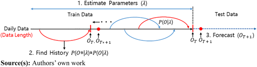
This study empirically investigates daily demand forecasting by examining the impact of data length within a structured catering service dataset. The analysis utilizes data from a large-scale catering service provider (Company A), which operates through major distribution centers to supply hundreds of dining plants nationwide. These plants provide meals – breakfast, lunch, and dinner – to various customer segments, including businesses, government offices, schools, and business complexes. To ensure representativeness, detailed operational data from five selected dining facilities were analyzed, capturing variations in meal time hierarchies and demand patterns. The dataset spans 24 months of daily meal records, which were segmented into six different data lengths for forecasting analysis, as illustrated in Figure 1.
Target: 14 daily meal data (morning, afternoon, and evening) at five plants.
Training Set: 24 months of meal data (730 days) from June 1, 2015 to May 28, 2017, classified into six different data lengths such as 1, 2, 3, 6, 12 and 24-month.
Test Set: daily meal data for 5 weeks from May 29 to July 2, 2017.
Estimates daily forecasts for the next 28 days (4 weeks).
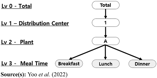
Furthermore, using the daily meal data of Company A, the hierarchy is set to the meal time of the plant based on the distribution center. These settings form a three-level hierarchy as shown in Figure 2. The hierarchy consists of meal time as the lowest level, followed by plant, distribution center, and finally total level. Use this hierarchy to generate forecast.
3.2 Application of forecasting methods
The study performs daily demand forecasting using Holt-Winters Exponential Smoothing Model (HW) and the Hidden Markov Models (HMM) across six different data lengths.
3.2.1 Holt-Winters exponential smoothing model (HW)
Holt-Winters Exponential Smoothing Model (HW) is a demand forecasting model that takes into account seasonality and trend in time series data, enhancing its accuracy. In time series data, there are two main types of seasonal variations: additive seasonal variation and multiplicative seasonal variation. In the case of time series data with additive seasonal variation, the seasonal component maintains a constant magnitude. On the other hand, for time series data with multiplicative seasonal variation, the magnitude of the seasonal component gradually increases or decreases in proportion to the underlying trend. This model consists of three equations and a forecasting equation, which smoothens three time series patterns: level, trend, and seasonality. The equations are structured as follows:
If time series data exhibits only a trend and no seasonality, Holt model is employed. This model forecasts by adding the trend to the level, and the initial values for trend and level are estimated through linear regression analysis.
3.2.2 The Hidden Markov model (HMM)
Determining the optimal number of hidden states in the Hidden Markov Model (HMM) is a critical step in model development. The number of states should be chosen to balance the model’s ability to adequately explain the observation sequence with maintaining manageable complexity. Information criteria, such as the Akaike Information Criterion (AIC) and the Bayesian Information Criterion (BIC), are commonly used for this purpose. These criteria evaluate models based on a trade-off between goodness-of-fit and model simplicity, as represented by the following equations:
K: Number of parameters in the model,
M: Data length,
L: Maximum likelihood value of the mode
The first term encourages a detailed fit to the data, while the second term penalizes excessive parameters, promoting model generalization. By minimizing the sum of these terms, the optimal number of hidden states can be determined. This approach ensures that the model effectively captures patterns in the time series while avoiding overfitting.
To apply this framework, the study draws on Hassan and Nath’s (2005) method for predicting stock prices using HMM. Their approach leverages likelihood values to calculate similarities between observation sequences. Given an observation sequence and a model , the likelihood is computed by summing over all possible state sequences consistent with the model. The forward algorithm is typically used for this computation. Based on their methodology, the next day’s stock price is predicted using the relationship:
In this study, we adopt a similar approach, using six different data lengths to estimate HMM parameters for daily meal demand forecasting. Specifically, Equation (5) is adapted to predict the next day’s meal demand based on data length and the differences between current and similar past observations.
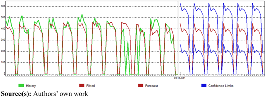
Figure 3 illustrates the overall procedure for predicting daily meal demand, detailing the steps of parameter estimation, sequence matching, and forecast. The analysis of six different data lengths provides an in-depth examination of how data length influences forecasting accuracy and efficiency. By comparing the results of traditional time series models with the proposed HMM approach, this study aims to demonstrate the superiority of HMM in capturing daily meal demand patterns.
3.3 Evaluation of forecast accuracy
The demand forecast results use Mean Absolute Percentage Error (MAPE) to analyze the accuracy of the forecast and suggest optimal data period. MAPE is a useful metric that allows you to compare the accuracy of any forecast, regardless of the unit or size of the product, expressed as a percentage error, as shown in the equation below.
To verify the accuracy of the forecast, we used out of sample test (Rolling Forecasting MAPE). This method involves cross-validating the performance and forecast values by moving the forecast time point by one week for five weeks starting in June 2017. The accuracy of the forecasting model was evaluated at each point in time using out of sample test. This is an important verification process to ensure that the proposed model is not limited to a specific point in time, but can be reliably utilized at various points in time. Therefore, out of sample test verifies the accuracy of the forecasting model, and we can conclude that the proposed model can be reliably utilized at various points in time.
Finally, considering the lead time of purchasing and production, the accuracy was measured using 14 days (2 weeks) of forecasts. For this purpose, we set the forecast interval to 2 and 3 weeks. The reason is that 1 week was not included in the forecast because it was already finalized as a purchase and production plan, and 4 weeks was excluded because it was outside the accuracy measurement range considering the short-term forecast of 14 days.
4. Empirical analysis
In this study, we applied Holt-Winters Exponential Smoothing Model (HW) and the Hidden Markov Model (HMM) to perform daily demand forecasting across six different data lengths. Forecast Pro Trac Software was used to analyze forecast accuracy hierarchically, determining the appropriate hierarchy level through a bottom-up approach across three levels of meal time (Yoo et al., 2022).
4.1 Forecasting results of Holt-Winters exponential smoothing model (HW) by data length
As shown in Table 4, the statistical analysis highlights the influence of data length on forecasting performance, evaluated through key metrics such as adjusted R-squared, MAPE, mean demand, and standard deviation. Longer data lengths, such as 24-month and 12-month periods, demonstrated stable mean demand values (137.41 and 139.90) and consistent variability (standard deviations of 85.82 and 86.20). These periods achieved adjusted R-squared values of approximately 71–72% and MAPE ranging from 16% to 17%, indicating their ability to capture long-term trends with moderate accuracy.
Within-sample statistics by data length
| Data length | Mean demand | Std. deviation | Adjusted R-squared | MAPE |
|---|---|---|---|---|
| 24-month (730 days) | 137.31 | 85.82 | 0.71 | 16.86 |
| 12-month (365 days) | 139.90 | 86.20 | 0.72 | 15.50 |
| 6-month (182 days) | 137.77 | 85.23 | 0.71 | 15.93 |
| 3-month (84 days) | 135.90 | 83.76 | 0.73 | 14.29 |
| 2-month (56 days) | 130.54 | 84.34 | 0.59 | 19.21 |
| 1-month (28 days) | 123.35 | 85.85 | 0.51 | 28.43 |
Source(s): Authors’ own work
In contrast, the 3-month data length exhibited superior performance, achieving the highest adjusted R-squared (73%) and the lowest MAPE (14.29%), while maintaining a mean demand of 135.90 and the smallest variability (standard deviation of 83.76). These results suggest that the 3-month data length offers the optimal balance between accuracy and efficiency.
However, shorter data lengths, such as 2-month and 1-month periods, showed significant declines in performance. Adjusted R-squared values dropped to 59% and 51%, respectively, while MAPE increased to 19.21% and 28.43%. This decline indicates that shorter data lengths are insufficient to capture meaningful demand patterns, leading to reduced forecasting accuracy.
Further empirical analysis of the Holt-Winters Exponential Smoothing Model (HW), as shown in Table 5, reinforces these findings. Forecasting with the 3-month data length yielded high accuracy, with Mean Absolute Percentage Errors (MAPE) averaging 12.11% and 11.65% for 2-week and 3-week forecast intervals, respectively. This demonstrates that the 3-month data length effectively captures demand patterns in the test set, reinforcing the conclusion that recent data provides reliable forecasts for the near future.
Out of sample test: forecasting results by data length (HW)
| Data length | MAPE | ||||
|---|---|---|---|---|---|
| Forecast horizon (week) | |||||
| 1 | 2 | 3 | 4 | Average (2 and 3 week) | |
| 24-month (730 days) | 13.54 | 13.85 | 13.50 | 13.69 | 13.68 |
| 12-month (365 days) | 13.82 | 14.28 | 13.95 | 14.05 | 14.12 |
| 6-month (182 days) | 13.94 | 14.23 | 13.99 | 14.08 | 14.11 |
| 3-month (84 days) | 13.06 | 12.11 | 11.65 | 12.58 | 11.88 |
| 2-month (56 days) | 16.44 | 16.58 | 17.24 | 16.51 | 16.91 |
| 1-month (28 days) | 18.18 | 18.35 | 20.53 | 18.27 | 19.44 |
Source(s): Yoo et al. (2022)
4.2 Forecasting results of the Hidden Markov model (HMM) by data length
As shown in Table 6, the forecasts based on the 3-month data length demonstrate very high forecast accuracy, with average Mean Absolute Percentage Errors (MAPE) of 12.3% for a 2-week forecast and 8.5% for a 3-week forecast.
Out of sample test: forecasting results by data length (HMM)
| Data length | MAPE | ||||
|---|---|---|---|---|---|
| Forecast horizon (week) | |||||
| 1 | 2 | 3 | 4 | Average (2 and 3 week) | |
| 24-month (730 days) | 17.82 | 36.18 | 6.93 | 10.21 | 21.56 |
| 12-month (365 days) | 14.36 | 11.48 | 10.65 | 10.50 | 11.07 |
| 6-month (182 days) | 12.41 | 11.89 | 11.04 | 14.33 | 11.46 |
| 3-month (84 days) | 9.58 | 12.30 | 8.50 | 19.45 | 10.40 |
| 2-month (56 days) | 10.34 | 19.08 | 14.66 | 10.48 | 16.87 |
| 1-month (28 days) | 16.94 | 13.72 | 22.06 | 13.68 | 17.89 |
Source(s): Authors’ own work
Similar to time series model, it was observed that forecasts based on shorter data lengths of 1-month and 2-month exhibited lower forecast accuracy. This is because with a shorter one, it becomes more challenging to adequately capture inherent patterns. Additionally, limitations can arise in finding the most similar likelihood values of recent performance in the short data, and over-forecasting or under-forecasting might occur when the subsequent values in the similar past performance data have the maximum or minimum values.
In contrast, forecasts based on longer data lengths of 6-month, 12-month and 24-month showed slightly reduced accuracy compared to the 3-month data-based forecasts. The reason for this is that, although longer data length provides a higher likelihood of finding the most similar likelihood values, significant changes in recent trends, such as a substantial increase in recent average meals from 200 to 300 compared to last year, may result in decreased forecast accuracy.
4.3 Forecasting results by data length (HW vs HMM)
Table 7 presents the average Mean Absolute Percentage Error (MAPE) for various data, measured using both Holt-Winters Exponential Smoothing Model (HW) and the Hidden Markov Model (HMM).
Out of sample test: forecasting results by data length (HW vs HMM)
| Data length | MAPE | |
|---|---|---|
| Forecast horizon: average 2 and 3 week | ||
| Holt-Winters model (HW) | Hidden Markov model (HMM) | |
| 24-month (730 days) | 13.68 | 21.56 |
| 12-month (365 days) | 14.12 | 11.07 |
| 6-month (182 days) | 14.11 | 11.46 |
| 3-month (84 days) | 11.88 | 10.40 |
| 2-month (56 days) | 16.91 | 16.87 |
| 1-month (28 days) | 19.44 | 17.89 |
Source(s): Authors’ own work
HMM displays higher forecast accuracy in all months except the 24-month data length when considering 2-week and 3-week forecast periods, as compared to HW. Additionally, forecasts based on relatively short data lengths of 1-month and 2-month consistently exhibited lower forecast accuracy. This is because shorter datasets make it more challenging to accurately estimate demand patterns. Conversely, as the forecast horizon lengthens, a trend of decreasing MAPE is observed. This indicates that as data length increases, the predictive capabilities of the model improve. However, the 24-month data length based on HMM showed significantly reduced accuracy compared to other forecasts.
Therefore, the 3-month data length is sufficient to maintain the efficiency and accuracy of the forecast, and we propose the 3-month one as optimal data length for daily demand forecasting. This seems to be the optimal period to maximize forecast accuracy, considering the cost and efficiency of data collection and analysis. However, these results are specific to the data used in empirical analysis and should be interpreted in that context.
5. Conclusions
This study analyzed the impact of data length on forecasting accuracy within horizontal data structures and proposed an optimal methodology for daily demand forecasting. By conducting both a theoretical review and an empirical analysis using time series model and Hidden Markov Models (HMM), the research demonstrated that longer data lengths do not necessarily yield better forecasting accuracy. Instead, appropriately adjusted data lengths can enhance both accuracy and efficiency, particularly in short-term demand forecasting.
The empirical findings indicate that the 3-month data length effectively balances accuracy and efficiency by capturing recent demand fluctuations and seasonal patterns while minimizing noise from excessive historical data. These insights have significant practical implications for businesses, aiding in daily operational planning, inventory control, and supply chain decision-making. Furthermore, this study highlights the importance of aligning forecasting models with business objectives, validating data integrity, and continuously assessing model performance using key evaluation metrics such as Mean Absolute Percentage Error (MAPE).
However, this research has several limitations that must be acknowledged. First, external factors such as macroeconomic conditions, policy changes, and unforeseen disruptions (e.g., labor strike, temporary holiday) were not incorporated into the model. As a result, the forecasting accuracy may decline in periods of significant environmental change. Second, the analysis was conducted within the catering service industry, limiting the generalizability of findings to other sectors. Future research should validate the proposed methodology across diverse industries, such as e-commerce, retail, and logistics, to enhance its applicability. Third, the sensitivity of HMM to key parameters, such as the number of hidden states and initialization conditions, presents challenges in broader applications, warranting further investigation. Finally, the study focused on short-term forecasting, leaving open questions regarding its effectiveness in medium-to long-term forecasting scenarios.
Despite these limitations, this research challenges conventional assumptions that longer historical data leads to more accurate demand forecasts. It provides a practical framework for improving forecasting efficiency in real-world applications. Future studies should explore alternative forecasting intervals (e.g., weekly or monthly), incorporate external influencing factors, and test the model under various operational settings to strengthen its robustness and real-world applicability.
This work was supported by Institute of Information & Communications Technology Planning & Evaluation (IITP) grant funded by Korea government (MSIT) (No.RS-2022-00155915, Artificial Intelligence Convergence Innovation Human Resources Development (Inha University)).
