
Planning interventions on urban infrastructure networks requires the consideration of costs of interventions and interruptions to the service provided by the infrastructure. It also requires taking into consideration how these costs and interruptions change due to the proximity of close networks. For example, it is less expensive to replace a gas pipe if the road is open, and, if a pipe is being replaced, there is a probability that the adjacent water pipe will be hit, resulting in a loss of service. Determining the optimal intervention programme for a single network is challenging as one has to consider all the objects within the network. Determining the optimal intervention programmes for multiple networks is even more challenging, particularly because the number of possible intervention programmes explodes. In this paper, the application of a unified model of the service provided by urban infrastructure networks to be used in the search for optimal intervention programmes on multiple networks simultaneously is presented. By using a single equation for all networks, the model enables an increase in the speed of calculation compared to traditional models, as a single equation can be used. The reductions in accuracy from more traditional models are discussed.
Notation
- Am
service on network m
- Ap
pipe diameter
- Bfric(t)
friction power at time t
- Bin(t)
input power at time t
- Bleak(t)
leaking power at time t
- Bloss(t)
lost service power at time t
- Bm
general service power on network m
- Bm
service power on network m
- Bm,in(t)
service power input for network m
- Bm,out(t)
service power output for network m
- Bout(t)
service output power at time t
- Brd,opt
traffic power in an optimal case
- Brd,out
traffic power in actual case
- boxcar(x,a,b)
boxcar function
- CLOS,el
monetised level of electricity service
- CLOS,gs
monetised level of gas service
- CLOS,rd
monetised level of road service
- CLOS,sw
monetised level of sewer service
- CLOS,wa
monetised level of water service
- Cm
service pressure on network m
- cfix,el
fixed cost of electricity production
- cfix,gs
fixed cost of gas production
- cfix,sw
fixed cost of sewer operation
- cfix,wa
fixed cost of water production
- closs,rd
additional cost of impossible trips
- cpoll,sw
per-unit cost of sewer overflow
- cprod,el
per-unit cost of electricity production
- cprod,gs
per-unit cost of gas production
- cprod,wa
per-unit cost of water production
- csell,el
per-unit revenue for electricity (as metered)
- csell,gs
per-unit revenue for gas (as metered)
- csell,wa
per-unit revenue for water (as metered)
- ctravel,rd
average travel time cost per hour
flow vector
- Dhyd
hydraulic diameter
- Dm
service flow on network m
- Dn,m
service flow through object o n,m
- Dη
service flow in/out of node η
- Em
service unit on network m
- f0,n,m
conductivity function of object o n,m at time 0
- fD
Darcy friction factor
- fM
Moody friction factor
- GLOS,m
cost occurred by the loss in the level of service for network m
- GLOS,m,fix
fixed cost of operating the network
- gprod,m
cost per service power unit produced
- grcv,m
revenue per service power unit received
- H(x)
Heaviside function
- M
network characteristic matrix
- m
index variable for the network m ∈ 1,…,M
- mij(with i = j)
sum of the conductance of all objects connected to node η i
- mij(with i ≠ j)
conductance between nodes η i and η j
- on,m
index variable for object n ∈ 1,…,N from network m
pressure vector
- Tgs
gas temperature
- Tω
index for the time phase with ω ∈ 1,…,Ω
- t
index for time
- Zgs
compressibility factor
- γn,el
electric conductivity
- γn,gs
gas conductivity
- γn,m
conductivity term for object o n,m
- γn,rd
road conductivity in the actual state
- γn,sw
sewer conductivity
- γopt,rd
conductivity of the road network in optimal state
binary intervention indicator variable
- ηi
index variable for the nodes η i ∈ 1,…,I
are the interactions received by object o n,m at time index ω from other objects
- ρ
fluid density
- σn,m
slimness term for object o n,m
- ω
time index
Introduction
Urban infrastructure networks such as electricity, gas, roads, sewage and water networks provide crucial services to the population. It is essential to keep these services at an appropriate level in order to provide a stable city life, which is linked to well-functioning infrastructure (UN-Habitat, 2013). In order to keep these services at an appropriate level, interventions have to be executed to ensure an appropriate state of the infrastructure network. These interventions, however, might themselves cause disturbances to the service. The task of urban infrastructure management is, therefore, to balance these two disturbances to find an optimum that fulfils all requirements, such as minimal service level and budget limitations. Because, in urban areas, infrastructure networks are in close proximity, interactions between networks can occur, but this closeness can also be used as an advantage in order to combine interventions on neighbouring objects, even of different networks. This, however, poses a challenging task regarding calculating the optimal intervention programme, as these interactions and closeness demand high computational power, as, traditionally, all different networks have their own methods of intervention programme calculation. In order to facilitate an ensemble calculation, a unified modelling approach is needed that can be used to model the different networks and their properties with appropriate accuracy. In this paper, such a modelling approach is presented.
Literature
The literature that provides helpful models can be split into two parts: (a) literature about single networks and (b) literature about definitions of level of service.
For the infrastructure networks investigated in this paper, literature on intervention planning can be grouped according to how the specific networks can be inspected. If it is possible to monitor the deterioration of an object (e.g. roads and sewers), the optimisation methodologies used are different to networks, where it is not possible to easily monitor deterioration (e.g. gas and electricity). For the former, the models usually are based on condition states, whereas, for the latter, the models are mainly based on probabilistic survival.
The literature is presented in tabular form in Table 1. In this table, the different network types, the considered objects, the optimisation goals (i.e. what is to be minimised/maximised) and the characteristics as well as the optimisation technique used and the result are presented. The last two columns list the simplifications and omitted characteristics in the respective models.
Intervention planning literature summary
| Author | Network | Object types | Optimisation goals | Considered characteristics | Optimisation technique | Result | Simplifications | Unconsidered characteristics |
|---|---|---|---|---|---|---|---|---|
| Arthur et al. (2009) | Sewer | Pipes | Framework only | Failure probability function, inspection data, network effects | Framework only | Optimal intervention programme | Scores instead of real values | Other networks |
| Louit et al. (2009) | Electricity | Conductors | Minimise cost, as in the study by Stillman (2003), maximise availability or maximise profit for the network operator | Budget limit, availability limit | Statistical estimation | Optimal time interval between interventions | Failure modes disregarded, fixed intervention policy, time-independent costs | Network effects, other infrastructure networks |
| Egger et al. (2013) | Road | Pavement layers | Minimise cost, maximise reliability and Pareto surface from both | Pavement design demand, traffic demand, actual pavement load | Genetic algorithm | Optimal intervention programme for one object | Only one intervention type | Network effects, other infrastructure networks |
| Egger et al. (2013) | Sewer | Pipes | Determine deterioration function | Failure probability function, inspection data, expert knowledge | Monte Carlo Markov chain | Deterioration function posterior distributions | Intervention programmes | |
| Dehghanian et al. (2013) | Electricity or gas | All | Maximise the condition-improvement-to-cost ratio | Failure probability, network reliability | Iterative method | Optimal strategy to construct an intervention programme | General level, no detailed methodologies given | Other infrastructure networks |
| Mathew and Isaac (2015) | Road | All | Pareto front for cost minimisation and condition maximisation | Road condition index, intervention types, condition index history | Genetic algorithm | Pareto front to calculate intervention programmes | Independent objects | Network effects, other infrastructure networks, grouping benefits |
| Zayed and Mohamed (2013) | Water | Pipes | Minimise sum of intervention costs and expected failure costs | Network simulation | Proprietary optimisation | Optimal clustered intervention programme | Objects independent | Network effects, other infrastructure networks |
| Lethanh et al. (2014) | Road | All | Minimise short- and long-term costs for users and road operators | Network structure, traffic configuration, spatial distribution | Linear programme | Optimal clustered intervention programme for 1 year | Linearisation, independence of work zones | Multiple years, other networks |
| Tscheikner-Gratl et al. (2016) | Water, sewer, road | Pipes/road section | Minimise criticality | Object condition, deterioration models, network configuration | Iterative method | Optimal clustered intervention programme | Interactions between networks, level of service |
The next part of the literature focuses on the different definitions of level of service on the five networks. For electricity networks, the level of service is based on ‘expected unserved energy’, as shown by Rietz and Sen (2006). They found that the most prominently used indicators are the loss of load probability and expected unserved energy. The loss of load probability is the probability of not being able to provide a certain power to a customer, regardless of the customers’ actual demand (i.e. this indicator does not take into account if, at the moment of power loss, the consumer is actually demanding power or not). The expected unserved energy amends this indicator by factoring in the expected energy demand. The determination of the costs related to this unserved energy is, however, possible only with an approximative approach as presented by Choi et al. (2006) and Reichl et al. (2013). For the gas network, the level of service definition is rather loose and more focused on minimum standards that have to be achieved, such as those of the Office of Gas and Electricity Markets (Ofgem, 2009). These standards ensure safety and reliability while also providing minima for service interruptions, pressure, flow and gas quality. For the road network, the definitions of level of service strongly depend on the viewpoint. From a traffic planner’s perspective, the level of service can be linked to the traffic flow (e.g. vehicles per hour and passengers per hour) such as in the papers by Bhargrab et al. (1999) and Yang and Bell (1998) or the ‘instantaneous driver utility’ presented by Kita (2000), although it is conceded there that the exact utility function may be hard to obtain. From the engineering perspective, the level of service is focused on the single object’s performance after an intervention – that is, the service (increase) is defined as ‘reduction of …’, as in the book by Astra (2003) or in a monetised form (i.e. ‘financial benefits due to reduction of …’), as in the paper by Adey et al. (2012). However, these indicators, in most cases, require the estimation of a non-zero baseline in order to estimate the reduction.
For sewer networks, the level of service is linked to the main function of sewers, namely the safe transport of sewage to the wastewater treatment plant, with the exact definition depending on local regulations and laws. In detail, the level of service can be linked to the risk of pollution costs (caused by overflow), as in the paper by Ashley and Hopkinson (2002), although the authors state that pollution costs are hard to define; sediment build-up, as in the paper by Gerard and Chocat (1999); or the full event chain of ‘defect–dysfunction–impact’, as presented by Caradot et al. (2011) and Le Gauffre et al. (2007). For the water network, the level of service can be seen from a ‘hydraulic power’ (i.e. the product of pressure and flow) point of view (Todini, 2000) or a resilience point of view – that is, based on the number of flow/pressure combinations that can fulfil the demand (Todini, 2000). The level of service is distinct for each network, and, even within one network, different definitions of level of service exist. They are all summarised in Table 2.
Level of service literature summary
| Author | Network | Level of service definition | Remarks |
|---|---|---|---|
| Rietz and Sen (2006) | Electricity | Loss of load probability, expected unserved energy | Assigned costs are unreliable |
| Choi et al. (2006) | Electricity | Expected unserved energy | Industry costs can be approximated |
| Reichl et al. (2013) | Electricity | Expected unserved energy | Approximation lacks data |
| Ofgem (2009) | Gas | Pressure, flow, reliability and safety | Minimal standards, but no real level of service |
| Yang and Bell (1998) | Road | Traffic flow (vehicles per hour, passenger per hour …) | Exact parameter depending on the investigated problem |
| Bhargrab et al. (1999) | Road | Function of nominal capacity, speed, road condition | Takes into account road condition directly |
| Kita (2000) | Road | Instantaneous driver utility | Drivers’ utility functions are hard to obtain |
| Yang et al. (2000) | Road | Function of maximum capacity | The maximum level of service is below the maximum capacity |
| Adey et al. (2012) | Road | Financial benefit due to reduction in user costs | The baseline for comparison is difficult to define |
| Astra (2003), NZ Transport Agency (2016) | Road | Reduction in … (multiple parameters) | The baseline for comparison is difficult to define |
| Gerard and Chocat (1999) | Sewer | Sediment build-up | Physical model |
| Ashley and Hopkinson (2002) | Sewer | Risk of pollution events | Pollution costs are hard to define |
| Le Gauffre et al. (2007) | Sewer | Defect–dysfunction–impact chain | Environmental impacts due to sewer condition |
| Caradot et al. (2011) | Sewer | Defect–dysfunction–impact chain | Number estimates for Le Gauffre et al. (2007) |
| Germanopoulos et al. (1986) | Water | Hygiene, pressure/flow, temperature | |
| Todini (2000) | Water | Hydraulic power | Energy balance approach |
| Todini (2000) | Water | Network redundancy | Flow/pressure combinations that can fulfil the demand |
In summary, it can be seen in Table 1 that most methodologies for planning infrastructure interventions lack consideration of other infrastructure networks or even other objects in the same network. In some methodologies, there is unidirectional consideration or consideration as a trade-off, but without network effects. The methodologies that account for network effects, however, do not account for multiple time steps. This gap could also have been amplified by the lack of a unified service model, as separate models for each network greatly increase the complexity of interaction calculations. The service, as summarised in Table 2, is distinct for each network, and, even within one network, different definitions of level of service exist.
Additionally, there exists a substantial amount of literature about interdependent networks, but more focused on the area of network vulnerability. Johansson and Hassel (2010) presented a model for the vulnerability analysis of interdependent infrastructure networks, which was extended by Trucco et al. (2012) to include the possibility to make the vulnerability analysis time dependent.
Guidotti et al. (2016) presented a modelling approach to express mathematically the dependencies for urban infrastructure networks, although the focus was on the resilience of critical infrastructure subject to hazard events (i.e. the amount of service that can be provided despite the event-caused failures).
So far, a methodology that combines intervention planning over multiple networks with multiple time steps and with consideration of the level of service is still lacking, also due to the different definitions of level of service.
Generalised service model
In this paper, a new level of service model is presented that builds on and extends the general model presented by Kielhauser et al. (2016), and demonstrates how it can be integrated into each network, in order to link them to the methodology presented by Kielhauser and Adey (2018).
The model is formulated in such a way that it can be applied to every network investigated with reasonable accuracy, so that an ensemble calculation is possible – that is, that all networks can be calculated using the same algorithm, with an accuracy that is sufficient for infrastructure maintenance planning.
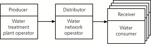
The service model is rooted in the following general classification of involved stakeholders on infrastructure networks, shown in Figure 1.

The producer is responsible for producing the ‘goods’ (e.g. freshwater, gas and electricity) demanded by the receiver. It is also possible that more than one producer exists. The distributor (i.e. the network operator) is responsible for the distribution of the goods – that is, ensures that the goods produced reach the receiver. It is also possible that two stakeholders are one entity (i.e. company). It might also be that the producer and receiver are the same entity – for example, on road networks. (Road users ‘produce’ a trip by wanting to go from A to B, and, if they arrive, the trip is ‘consumed’. This will be discussed in detail in the appropriate section later on.) All three stakeholders not only influence the transport (i.e. flow) of the goods on the network, but also benefit from the network in one way or the other. The producer can distribute the goods on the network and sell it to the receiver. The receiver benefits from the service and pays the producer for it. The distributor keeps the network in such a state that the distribution from producer to receiver is functioning (i.e. the network is functioning) and charges the producer, the receiver or both for providing an adequate level of service on the network. Certainly, it is possible to use a different subdivision of stakeholders. e.g. the ‘receivers’ of a network can e.g. be subdivided into ‘private customers’ and ‘public customers’ (which can further be divided into e.g. ‘hospital’ and ‘police’). However, for ease of understanding, the presented subdivision is used in the next sections.
Using the terminology from the paper by Kielhauser et al. (2016), the service on a network can be described by the same schematic expression: a time integral of the flow of the good/service/units in/on the respective network m. This is necessary to be able to combine all networks in one mathematical expression in order to facilitate the ensemble calculation between the networks. In order to facilitate understanding, the terminology is described here briefly. In these networks, however, the naming and usage of variables are not consistent across networks – that is, sometimes the same word or variable is used to mean different things on different networks. For example, the variable Q is used for charge in electrical engineering, but for flow in hydraulic engineering. Therefore, in the presentation of the mathematical model, the variable names have been changed to A,B,C,… in the order of their appearance to avoid confusion. The following basic equation shows the schematic expression of the service A
In order to simplify explanations, the following terms are introduced
service power Bm: the derivative of the provided service with respect to time – that is, the service per time unit
2service pressure Cm: the quotient of service power and service flow Dm
3service flow Dm: the amount of service units that flows through a given cross-section per unit time
4service unit Em: the product of service flow and time.
5
From Equation 1, it can be seen that the service provided is an integral of service power over time. Therefore, the loss of service can be measured using the same integral. In general, loss of the level of service occurs due to the condition of the objects and the implications caused by this (leaks, resistance, partial closure, rerouting etc.). On a network, this can be depicted as:
The network shown in Figure 2 consists of two producing nodes η1 and η2; one intermediate node η4; and three consuming nodes η3, η5 and η6. These nodes are linked by the objects o1 to o6.
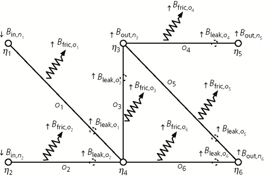
In nodes η1 and η2, there is a service power input Bin(t), and, in η5 and η6, a service power output Bout(t). During the transmission of the service power, there is the possibility of Bfric(t) friction along the objects, η3, which represents a loss of service power that is related to the length of the object. Additionally, there is also a possibility of leaks Bleak(t) on the objects, where service power may also be lost. In this case, the loss is related to a loss of service units. The sum of Bfric(t) and Bleak(t) is referred to as lost service power Bloss(t). For the system to be in balance, the following equation holds true
By examining Equation 6, it can be seen that the infeed service power is to be shared between the network (where it has to compensate for the losses) and the output. If the network, which, due to an increasing Bloss in the network, consumes more service power than expected, this leads to less output service power Bout, assuming that the input Bin stays constant. On the other hand, if the input Bin decreases (with the loss over the network Bloss being unchanged), the output service power also decreases. Normally, both will happen simultaneously. First, if the network consumes more service power (due to friction, leakage etc.), the producer increases the infeed service power to compensate for the losses and to supply a constant level of service. At some point, the maximum production capacity will be reached. Thus, a further increase in network losses will lead to a loss in the level of service, as the infeed service power will be constant, but the loss will increase.
With the loss of service defined in terms of service power, the service power state and the loss of service power can be estimated for each network. To facilitate reading, the index (t) for each time point has been omitted. Following basic physical relations, the general form of the service power equation is
with γn,m as the conductivity term for object on,m; σn,m as the object slimness; Dn,m as the service flow through object on,m; and Bm as the service power in network m.
As presented by Kielhauser et al. (2016) and Kielhauser and Adey (2018), the full equation for γn,m can be written as
with γn,m(t) as the conductivity of object on,m at time t; f0,n,m as the conductivity function of object on,m at time 0; fω,n,m as the conductivity function of object on,m at time index ω; H(x) as the Heaviside function; as the interactions received by object on,m at time index ω from other objects; as the binary variable indicating if an intervention is executed on object on,m at time phase Tω; and boxcar(x,a,b) as the boxcar function, defined as
With this equation, the conductivity of the object can be described formally, on a per-object basis, allowing for distinct conductivity functions for each object that can also be fundamentally different (i.e. from different functional families such as exponential and rational) as long as the function is monotonically decreasing over time. Additionally, the interdependencies between the networks are taken into account by an interaction variable. The full details can be found in the paper by Kielhauser and Adey (2018), but, to summarise, it can be stated that, with the interaction variable, it is possible to account for functional (e.g. pumps that are electrically powered) and spatial (e.g. a water pipe break also affects the road above it) interdependencies, on an object level, with different interactions at different time phases. For the full description of the calculation of the interaction variable, please refer to the paper by Kielhauser and Adey (2018).
With the general definition given, the flow equation for all networks together can be rewritten as
with M as the network characteristic matrix; as the pressure vector; mij (with i = j) as the sum of the conductance of all objects connected to node (i ∈ 1,…,η); mij (with i ≠ j) as the conductance between nodes i and j (i, j ∈ 1,…,η); Dη as the current flowing in/out of node η; and as the flow vector. The conductance is simply the ratio of every object’s conductivity to its slimness. The network characteristic matrix is able to represent the structure of the network topology, including flow direction or different directional capacities. The network characteristic matrix also allows disconnected ‘subparts’ of the network, which, in the context of this paper, can be used to join all five investigated networks into one single matrix while still keeping them separated in their properties. This allows the whole calculation to be executed in one matrix operation, which substantially decreases calculation time.
Solving for and inserting into Equation 7, the service power over time can then be calculated. With addition of costs to this model, the (monetised) level of service (and the loss thereof) can now be defined as
with GLOS,m as the costs occurred by the loss in the level of service for network m; GLOS,m,fix as the fixed costs for operating the network; Bm,in(t) as the service power input for network m; Bm,out(t) as the service power output for network m; gprod,m as the costs per service power unit produced; and grcv,m revenue per service power unit received.
In other words, the loss in the level of service is expressed as the difference between the sum of the fixed costs plus the per-unit service power generation cost minus the service power revenue per service power unit received. In the next section, it is demonstrated how this model is applied to five different urban infrastructure networks.
Example use
In this section, it is demonstrated how the model presented in the section headed ‘Generalised service model’ can be interpreted for each type of network found in an urban area. First, the stakeholders of each network are shown, followed by a service definition. Then, the adapted form of Equation 11 is presented, to demonstrate how the model ties in with the general formulation.
Electricity
The urban electricity network is a potential network (i.e. a network where the flow is caused by potential differences between the nodes) that consists primarily of two object types: (a) conductors (longitudinal objects) and (b) point-like objects (such as substations, transformers, switches, voltage regulators and monitoring systems). These components have to function as a whole system to provide the service of electric power to the customers. In the process of providing the service, there are three stakeholders involved, which are shown in Figure 3.
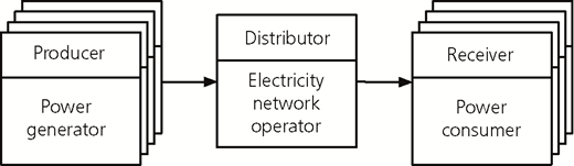
The first stakeholder is the producer group, which consists of power generation companies, which run power plants. These plants can be located not only in the vicinity, but also at greater distances and are connected through a wide-area grid. Both are connected to local substations, which provide the infeed point to the urban electricity network. This stakeholder group can (and has to) adapt permanently the generated power to the demand to keep the network in balance (i.e. prevent exceedance of the operating limits).
The second stakeholder is the distributor – that is, the entity that operates the distribution network. It is this stakeholder’s responsibility to keep the network in a state that allows the distribution of the generated power to the consumers with an acceptable level of losses, due to both the state of the network (e.g. resistive losses on the conductors, transformation losses and power factor) and the performed maintenance (i.e. service interruptions due to interventions or fault-caused interruptions due to inadequate/insufficient maintenance).
The third stakeholder is the consumer group, which consists of both private and industrial (i.e. large-volume) customers. The consumers use the generated and distributed power and pay for the received service. The payment is then split up into a network fee and a generation fee. There are different types of contracts that specify exactly the service that should be provided to the customer. The main component of these services is a guaranteed maximum current, as well as certain voltage limits that have to be kept. For example, a customer can order a connection of 125 A at 230 V ± 5%. This gives a power of 125 × 230 = 28·75 kW. For industrial customers, there can be additional terms in the contract, which, for example, allow load-shedding (i.e. allow disconnection of the industrial customer under certain circumstances in exchange for lower fees). As a general summary, it can be said that contracts (and with that the definition of service) for private customers are more or less standardised, with only the connection current being the adjustable value, but, for industrial customers, the contracts are much more specified and tailored to the actual industrial application of electricity (i.e. if the production process allows for temporary power outages, if a high availability level is needed etc.). However, for both customers, the core part is a specified current at a specified level of voltage – that is, a certain level of power (as power is the product of voltage and current). The level of service for an electricity network can be defined as
the ability to provide the consumer with a specified level of power at a specified level of voltage.
An adequate level of service is thus the ability to provide this specified level of power at the specified level of voltage to all consumers, and an inadequate level of service is the inability to do so. A loss in level of service is the difference between the desired level of service and the provided level of service.
There are multiple reasons that a loss in the level of service can occur. They can be attributed to either the producer or the network operator (in many cases, this is also the same organisation, so that one organisation is responsible for both power generation and distribution). On the production side, a loss in the level of service can be due to insufficient power generation (in terms of voltage and/or current, as power is the product of both) to provide the desired level of service. On the distribution side, the loss in the level of service can be caused by the state of the network – that is, the condition of the conductors and switches or whether a conductor is out of service due to failure or due to an intervention. A conductor being out of service changes the network configuration and causes either the current flow to be redirected, changing the voltage and current levels in the network, or, if consumers are connected only by out-of-service conductors, the consumer to be totally disconnected from the network. The losses due to non-optimal conductor condition can mainly be attributed to stray currents, which are dependent, among other things, on the insulation around the conductors.
As the model is based on an energy approach, for electricity networks the conductivity γ n,elec is purely the electric conductivity. The equation for the level of service, therefore, can be written as
with C LOS,el as the monetised level of electricity service; c fix,el as the fixed cost of electricity production; c prod,el as the per-unit cost of electricity production; and c sell,el per-unit revenue for electricity (as metered).
Gas
The urban gas distribution network is, like the electricity network, a potential network with two object types: (a) longitudinal objects (pipe sections) and (b) point-like objects (such as valves, compressors and meters). These objects have to function as a whole system to provide the service of energy to the customers. In the process of providing the service, there are three stakeholders involved, which are shown in Figure 4.
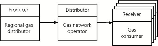
The first stakeholder is the regional gas distributor, which acts as a ‘producer’ by feeding in gas from the pressure reduction stations of the regional gas network into the urban gas network. The regional gas network receives the gas from international transmission lines, gas storages or local production. This stakeholder can (and has to) adapt the pressure and volume flow coming from the regional network in order to keep the pressure within an acceptable range, preventing both excessive pressure (which can lead to pipes bursting) and insufficient pressure, causing undersupply. However, as the focus here is on urban infrastructure networks, the regional gas distribution network is not considered.
The second stakeholder is the distributor – that is, the gas network operator. It is this stakeholder’s responsibility to keep the network in a state that allows the distribution of the gas to the consumers with minimal leakage and an acceptable level of pressure losses, due to both the state of the network (e.g. pipe fittings and wall corrosion) and the performed maintenance (i.e. service interruptions due to interventions or fault-caused interruptions due to inadequate/insufficient maintenance). The third stakeholder is the gas consumer group, which consists of both private and industrial (i.e. large-volume) customers. The consumers use the supplied gas to generate heat and pay for the received service. The payment is then split up into a network fee and a mass fee (i.e. a fee per supplied mass of gas, calculated though a volume proxy). There are differences in the types of contracts that specify exactly the service that should be provided to the customer. The main component of these services is a guaranteed minimum amount of mass flow, as well as a certain minimum pressure. For example, a customer can order a connection of 7 kg/h at 23 mbar. The level of service for a gas network can be defined as
the ability to provide the consumer with a specified mass flow at a specified pressure level.
An adequate level of service is when the ability to provide a specified level of mass flow at a specified level of pressure is greater than required. An inadequate level of service is when the ability to provide a specified level of mass flow at a specified level of pressure is lower than required. A loss in the level of service is the difference between the desired level of service and the provided level of service. There are multiple reasons that a loss in the level of service can occur. They can be attributed to either the producer (i.e. the regional gas distributor or their supplier) or the network operator (in some cases, this is also the same company, so that one utility company is responsible for both gas procurement and distribution). On the production side, a loss in the level of service can be caused by insufficient gas production or gas import (which can also be influenced by the international trade situation) to provide the desired amount of gas or by problems in pressure regulation. On the distribution side, the loss in the level of service can be caused by the state of the network – that is, the condition of the pipes, valves and pressure stations or whether a pipe is out of service due to failure or due to an intervention. A pipe being out of service changes the network configuration and causes either the gas flow to be redirected, changing the pressure and flow levels in the network, or, if consumers are connected only by out-of-service pipes, the consumer to be totally disconnected from the network. The losses due to non-optimal pipe condition can mainly be attributed to corrosion-caused leaking and internal friction of the transported gas.
For the gas network, the conductivity term is different, as the conductivity is dependent on more terms: , with f M as the Moody friction factor; Z gs as the compressibility factor; T gs as the gas temperature; and A p as the pipe diameter. It might seem unusual to combine these well-known terms into a term called ‘conductivity’, but this enables the ensemble calculation and is just a regrouping of terms.
The equation for level of service can be written as
with C LOS,gs as the monetised level of gas service; c fix,gs as the fixed cost of gas production; c prod,gs as the per-unit cost of gas production; and c sell,gs as the per-unit revenue for gas (as metered).
Road
The urban road network is, unlike the other networks, not a potential network in a physical sense, as the flow on the road network depends on individual decisions made by the vehicle drivers. The urban road network consists mainly of road sections (i.e. longitudinal objects). However, there are also objects such as tunnels, bridges or underpasses that add to the plurality of the objects in a road network. These objects have to work together as a whole system to provide the service of mobility to the road user. In the process of providing the service, however, there are only two stakeholders involved, if the logic of the section headed ‘Introduction’ is followed, which are shown in Figure 5.

The first stakeholder is the road user, which acts as both a producer and a receiver of the service of mobility. The road user has the desire to perform a trip from point A to point B in the road network, and, as soon as the road user reaches the destination, the mobility is ‘received’.
The second stakeholder is the road network operator. It is this stakeholder’s responsibility to keep the network in a state that allows road users to perform a trip in an acceptable amount of time, due to both the state of the network and the performed maintenance. However, as most infrastructure networks are buried underneath the road network, a significant source of network delays is caused by the interventions executed on other infrastructure networks, which impedes the mobility of the road users.
In that sense, the level of service can be defined as
the ability of a road user to reach any point in the road network from any other point in the road network in a reasonable amount of time
for example, with an average speed of 20 km/h. An adequate level of service is when road users have the ability to travel from all origin nodes to all destination nodes within specified amounts of times. An inadequate level of service is when this is not the case. A loss in the level of service is the difference between the desired level of service and the provided level of service. There are multiple reasons that a loss in the level of service can occur. These can be an inability to reach certain points on the road network or an excess travel time to reach the destination – that is, a reduced average speed. The inability to reach certain points is due to closed roads, which lies only in the sphere of the network operator. The excessive travel time is due to congestion, which is dependent on both the road users and the network operator. A poor road condition can lead to a decrease in possible speed on that road, and road closures, when they do not cut off certain nodes in the network, can lead to changes in traffic flow in the network, which can also cause congestion. Additionally, road users also contribute to traffic congestion through their route choice.
For the road, the conductivity term seems unusual at first, so an in-depth explanation is given. The service is mobility. Therefore, the mobility power represents the ability of the system to transport vehicles, given as mobility per second – that is, the desired number of vehicles that want to go at a certain speed [vehicles × metres/seconds]. Therefore, the conductance is given in [metres], and thus the conductivity (conductance divided by slimness [metres/1]) is given as γ n,rd : [metres/metres]. This road conductivity expresses the ratio of the real length to the apparent length of the road due to the non-perfect condition. This apparent length represents the loss of speed one occurs due to non-optimal road condition, but, instead of being expressed as a reduction in speed, it is expressed as the additional length one has to travel at the desired speed.
For the road network, therefore, the cost is related to the additional travel time instead of production costs
with C LOS,rd as the monetised level of road service; c travel,rd as the average travel time cost per hour; c loss,rd as the additional costs for impossible trips; B rd,opt as the traffic power in the optimal case (i.e. no closed roads); B rd,out as the traffic power in the actual case (i.e. with closed roads); γ opt,rd as the conductivity of network in the optimal state; and γ n,rd as the conductivity of the network in the actual state. In the first integral, the travel cost is calculated as the travel cost for the optimal network (first expression, where the mobility is calculated with a perfect network, i.e. where all trips are possible and executed on a network in perfect condition) augmented with two factors: (a) the first expression after the ‘1 +’, which calculates the rate of possible trips on the perfect network compared to the actual possible trips due to closed objects (note the different indices in the numerator), which considers the impossible trips due to network condition, and (b) the last expression in the first integral, which compares the actual possible traffic on an optimal network to the actual possible traffic on the actual network (i.e. considers only the possible trips, but with the actual road condition compared to an optimal one). The last integral adds additional costs for those trips that are totally impossible.
Sewer
The urban sewer network is, like the electricity network, a potential network, but with the difference that it is in most cases gravity controlled. In sewer networks, there are mainly longitudinal objects (pipe sections), but also, in some cases, there are point-like objects such as pumps or weirs. These objects have to function as a whole system to provide the service of wastewater collection to the customers. In the process of providing the service, there are two stakeholders involved, which are shown in Figure 6.
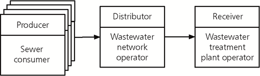
The first stakeholder is the ‘producer’ of wastewater, who is the customer of the wastewater disposal service. The customer produces wastewater and pays the wastewater disposal company to dispose of the resulting wastewater. Contracts with customers are, however, rare, as a connection to the wastewater system is normally prescribed by municipality laws, and the fee is part of the municipality taxes.
The second stakeholder is the wastewater disposal company, which acts as both a network operator and a receiver of the occurring wastewater. The disposal company has to keep the network in a state that allows collecting the wastewater from the customers with acceptable leakage and an acceptable level of flow capacity in order to transport the occurring wastewater safely to the wastewater treatment plant, due to both the state of the network (e.g. leakage, wall corrosion and sediment build-up) and the performed maintenance. The wastewater treatment plant, as the receiving end of the network, has to be able to accept all incoming wastewater and treat it according to local regulations. In that sense, the level of service can be defined as
the ability to transport securely (i.e. not exceeding the allowable leakage) a specified amount of wastewater mass of the connected customers to the wastewater treatment plant
and treat it accordingly.
There are multiple reasons that a loss in the level of service can occur. These include leaks in the pipes, stoppages in the pipes and exceeding the capacity of the water treatment plants. However, although leaks can be detected, it is hard to determine an actual leakage rate (in terms of a specific number) that can be used as a threshold. For the sewer network, just as for the gas network, the conductivity term is just a rearrangement of the well-known formulas: , with f D as the Darcy friction factor, ρ as the fluid density and D hyd as the hydraulic diameter, with only the Darcy friction factor being dependent on deterioration and improvement due to interventions. The level of service equation for the sewer network can be written as
with C LOS,sw as the costs of the level of sewer service; c fix,sw as the fixed cost of sewer operation; and c poll,sw as the cost per cubic metre sewer overflow. As for sewer networks, the typical way of billing is not dependent on the amount of produced sewage, and the static fees are simply included in the fixed costs. The remaining costs are those attributed to sewer overflows.
Water
The urban water distribution network is, like the electricity network, a potential network with two object types: (a) pipe sections and (b) point-like objects, for example, valves. These objects have to function as a whole system to provide the service of water to the customers. In the process of providing the service, there are three stakeholders involved, which are shown in Figure 7, but only two entities.
The first entity is the water supplier, which acts as both a producer, by treating freshwater from different sources, and then in the stakeholder role of the distributor, by distributing the treated water to the customers in the city. On the production side, the water supplier can increase the produced volume or the pressure in order to compensate for losses in the distribution network. The distribution network has to be kept in a state that allows the distribution of the water to the consumers with acceptable leakage and an acceptable level of pressure losses, due to both the state of the network (e.g. pipe fittings, wall corrosion and lime build-up) and the performed maintenance (i.e. service interruptions due to interventions or fault-caused interruptions due to inadequate/insufficient maintenance). However, the water supplier has more freedom to move the focus between countermeasures and interventions, as both are executed by the same company.
The second stakeholder is the consumer group, which consists of both private and industrial (i.e. large-volume) customers. The consumers use the supplied water for drinking purposes, but mainly for rinsing and cleaning purposes, as the major amount of the used water serves hygienic purposes. Therefore, the water has to conform to chemical, physical and microbacteriological standards to fulfil the consumers’ needs. An adequate level of service is when
the ability to provide the consumer with a specified water flow at a specified pressure level
is above the specified threshold. There are multiple reasons that a loss in the level of service can occur. On the production side, a loss in level of service can be caused by the producer not being able to fulfil the demand – for example, if there is a water shortage. On the distribution side, the loss in level of service can be caused by the state of the network – that is, the condition of the pipes and valves or whether a pipe is out of service due to failure or due to an intervention. A pipe being out of service changes the network configuration and causes either the water flow to be redirected, changing the pressure and volume flow levels in the network, or, if consumers are connected only by out-of-service pipes, the consumer to be totally disconnected from the network. The losses due to non-optimal pipe condition can mainly be attributed to leaks and internal friction. One thing that has to be noted about leaks, though, is that a certain amount of leakage is common and also accepted for water networks. If the acceptable amount of leakage is exceeded, an intervention is executed. In that sense, this can also be seen as a binary decision, however with a certain amount of leakage as an unacceptability threshold.
In the scope of maintenance of a distribution network, the focus is put only on pressure/flow, as hygiene is mainly in the sphere of the producer (by adequate water sanitation) or network designer (by ensuring adequate hydraulic residence time due to network layout), and temperature can be easily influenced by burying depth, which is also in the sphere of the network designer. Only pressure/flow depends on the state of the network and therefore within the scope of this model.
As both the water and sewer networks are hydraulic networks, the conductivity term for the water network is the same as for the sewer network. With this, the level of service equation for the water network can be written as
with C LOS,wa as the monetised level of water service; c fix,wa as the fixed cost of water production; c prod,wa as the per-unit cost of water production; and c sell,wa as the per-unit revenue for water (as metered).
Conclusion
In this section, conclusions are highlighted in order to show the benefits and limitations of the proposed model in contrast to those of traditional calculation methods.
The calculation of loss in the level of service in the methodology is based on the assumption that the loss in the level of service is proportional to the service provided through the network, plus additional fixed costs. As has been shown in the literature review, there are many different ways of quantifying the service (and the loss thereof), depending on the reference frame. Many of the presented ways can, however, be broken down into a part proportional to the provided service and a second ‘fixed’ part. Nevertheless, there are certain aspects of service definitions that are dependent on other parameters – for example, service definitions based on the accident rate on roads or chemical parameters in the water network. By amending the service equations, this can be accounted for as well, although this has not been done here.
The assumption of the conductivity being represented by a smooth decreasing function (if neither interventions nor interactions are present) (see the paper by Kielhauser et al. (2016) for more details) relies on the fact that ageing leads only to a decrease in the network-specific flow. However, for the water network, this is not necessarily true in all cases. If the chemical parameters of the water change (e.g. a shift in the pH value), the water can start as limestone-depositing, but with a shift in pH value, the limestone can then be re-solved in the water, thus effectively increasing the inner diameter again, which could lead to higher conductivity. However, if this level of detail is investigated, the actual roughness of the pipe inside, as well as other effects, should also be considered.
In the methodology, the flow in the networks is calculated based on the conductivity. For all networks except the road network, this represents the physical facts (however, with different names for conductivity in each network and in some cases the need for rearranging the equations). For the road network, this assumption requires a Wardrop-type equilibrium in the network, which is only an approximation. The real flow in the road network is hard to calculate, as it is dependent on the decisions of the drivers of the vehicles. Nevertheless, approximations of road traffic flow on the network are used due to their shown applicability and utility, so this approach is also followed in this methodology. For the other networks, the conductivity is physically present, although there is always the possibility to go into more detail, where the simple conductivity is not enough and local, small-scale phenomena play a non-negligible role.
This paper also touches briefly on the interactions between the networks and shows where they are accounted for. However, due to the complexity of interactions between networks, for the actual calculation of the interaction terms, it has to be referred to the paper by Kielhauser and Adey (2018).
In the methodology, a single equation is used for all service types on the network. On one hand, by using a single, generalised equation, it is possible to compare services across different types of infrastructure networks, and with that, a system-of-systems approach is feasible. On the other hand, a generalisation always asks for either simplification or otherwise an expansion of the existing equations. For example, water flow is usually modelled as incompressible flow, whereas gas flow is not. An equation that encompasses both either (a) has to simplify gas as being incompressible or (b) has to add a (at least for water unnecessary) compressibility term. The same logic is true for the other networks. Thus, using a combined model always is accompanied with either reduced accuracy or increased calculation time. At this point, there has to be an assessment whether the model with the reduced accuracy is sufficient for the question to be answered or if a higher accuracy, albeit with increased calculation time, is necessary. Depending on the task and accuracy/speed needed (e.g. a city-level assessment or cross-sector assessment), either one of the two approaches should be selected.
In particular, a high-level view on the state of the infrastructure – for example, as part of governance measures – benefits in practice from this methodology. Additionally, with the use of more detailed functions, it is possible for infrastructure-managing organisations that own or operate multiple networks to create benefits by planning interventions on different networks at the same time, thus reducing intervention cost as, for example, set-up costs can be shared, and at the same time increasing performance, as, due to combined interventions on a functionally interdependent network, parts require only one service interruption instead of two.
Future research in this area is to be focused on a real-world case study, verifying the use of this model with real-world assessments of the value of lost service, the inclusion of priority contracts and the development of improved cost/price models for sewer and road networks.
