
Interventions on infrastructure networks are required to ensure that they continue to provide the service expected of them. Although all existing methods for determining intervention programmes take into consideration, in some form, the costs and benefits associated with the interventions, there is a wide variation in exactly how it is done. With increasing strides to digitalise the determination of optimal intervention programmes, a systematic and quantitative method for determining their net benefits is required. The novelty in the proposed method is how the provided service and intervention costs over time are considered when determining optimal intervention programmes. It considers the difference between candidate intervention programmes and a reference intervention programme. In other words, it makes clear whether network-level considerations – for example, network-level synergies and constraints – should result in the intervention on an asset being executed earlier or later than indicated by the optimal asset life cycle. The method enables the use of advanced operations research algorithms in infrastructure-management systems and, therefore, helps enable the automated generation of optimal intervention programmes. For illustration, the method is used in the determination of the optimal intervention programme for a small railway network.
Notation
- CIP
cost related to the execution of the intervention programme IP
- Cref
cost related to the execution of the reference intervention programme
- cr(t)
cost of routine maintenance at time t
- cs(tperiod)
asset condition at the end of the planning period
- d
discount rate
- r(t)
risk related to failures at time t
- Sbeyond
service provided beyond the planning period
- SIP
service provided of the intervention programme IP
- Slong-term
service provided in the long term
- Speriod
service provided during the planning period
- Sref
service provided of the reference intervention programme
- ΔC
difference in the cost
- ΔS
difference in the service provided
Introduction
Managers of transportation infrastructure networks must plan and execute interventions – for example, rehabilitation and renewal interventions – on their infrastructure networks over time to ensure that they continue to provide the required service. The planning of these interventions normally requires the development of intervention strategies and the determination of intervention programmes (Adey, 2019). The intervention strategies define how individual assets or a group of assets should ideally be managed in the long term – that is, maintained and renewed. This refers to the determination of optimal asset life cycles considering the asset deterioration and the service provided over time. The intervention programmes define which interventions are to be executed in the next planning period based on the strategies and the state of the assets. There, network-level dependencies between the executions of interventions on multiple assets are taken into consideration. Interventions may be required earlier or later than proposed by the optimal asset life cycles due to limitations raised through network-level constraints. Further, synergies between assets due to network-level considerations may make an earlier or later execution of an intervention beneficial over the intervention according to the optimal asset life cycle. The optimisation of intervention programmes requires a method for evaluating individual programmes so that they can be compared with each other. This method needs to include the effects of the network-level synergies and constraints – that is, the impact of executing interventions out of their individual optimal point in time.
Over the past decades, specific infrastructure-asset-management systems have been developed for different transportation infrastructure or engineering structures to support infrastructure managers in intervention planning. These management systems enable, among others, the determination of intervention programmes. They differ significantly in how the network synergies and constraints are considered and in the methods used to quantify and evaluate different intervention programmes. The systems for railways normally enable the determination of intervention programmes specifically considering network-level synergies between interventions – that is, reductions in costs due to grouping interventions close to each other. They evaluate intervention programmes based on costs and proxies such as availability and reliability. The systems for roads and bridges most often determine intervention programmes with a focus on the prioritisation of interventions under limited resources. The incremental benefit/cost ratio is thereby a commonly used method. The benefit of a single intervention is quantified as the difference in the impacts when the intervention is executed and when it is not. None of the systems allows the determination of intervention programmes consistently considering the impacts of executing an intervention earlier or later than intended by the optimal life cycle of the assets. Nor do the assessed systems consider the impacts of executing an additional intervention that may be beneficial due to synergies with other interventions.
Further, neither the methods used in existing infrastructure-management systems nor the methods used in models developed in research do consistently quantify the costs and benefits considering how the infrastructure is managed beyond the planning period of the intervention programme. This is an important aspect, as interventions on transportation infrastructures have usually impacts that last longer than the planning period of an intervention programme. The most common approaches either neglect all impacts beyond the planning period, consider a residual value based on the asset condition at the end of the planning period or compare the impacts of an intervention during the extended asset lifetime without executing any intervention during this time. Others estimate the impact of executing an intervention in an intervention programme using the same approach as in developing asset life cycles, where all impacts of an asset life cycle are related to the length of the life cycle. This implies that a change in the current asset life cycle is going to be adapted in future life cycles, which confuses the determination of intervention programmes with the development of intervention strategies.
In this paper, a method is presented for systematically quantifying the net benefit of an intervention programme. The net benefit is defined in relation to the optimal asset life cycle as the difference in the provided service and the intervention costs of a candidate and a reference intervention programme. The systematic quantification of the net benefit enables the determination of whether the intervention on an asset within the planning period should be executed as indicated by the optimal asset life cycle or an earlier or later execution is worthwhile. It considers thereby the limitations and synergies raised through network-level considerations – for example, budget constraints or discounts due to the simultaneous execution of the interventions. The provided service beyond the planning period is considered by considering that the assets are managed beyond the planning period according to their individual optimal life cycles. Through its systematic approach, its direct relation to the optimal asset life cycles, and its ability to combine and compare the impacts of interventions on different asset types within an infrastructure, the method enables the use of advanced operations research algorithms to determine optimal intervention programmes within the digitalisation of infrastructure management. The method is used to determine the optimal intervention programme for a fictive example. Even though the example relates to a railway infrastructure, the methodology can be equally applied on other transportation infrastructures.
The remainder of the paper is structured as follows. First, an overview of the state of the art in asset-management systems and research is provided. Second, it is described how intervention programmes are developed by a consistent quantification. Third, the consistent quantification is illustrated on the example. Lastly, the paper is concluded.
Considering costs and benefits in the determination of intervention programmes
Infrastructure-management systems in practice
Over the past decades, many infrastructure-management systems have been developed that support infrastructure managers in determining intervention programmes. Table 1 provides an overview of some examples of infrastructure-management systems and states the methods used to evaluate intervention programmes. The list of mentioned management systems may be incomplete but contains the state of the art in infrastructure-management systems while covering the different methods currently used in practise. For further overviews of management systems, the reader is pointed to specific literature (Innotrack, 2007; Mirzaei et al., 2012; Mizusawa, 2009).
Infrastructure-management systems in practice
| Name | Infrastructure | Method used | Reference |
|---|---|---|---|
| HDM-4 | Road | Incremental benefit/cost ratio | Kerali et al. (2006), Odoki and Kerali (2006) |
| RED | Road | Incremental benefit/cost ratio | Archondo-Callao (1999) |
| SMEC-PMS | Road | Incremental benefit/cost ratio | Bartlett and Shirey (2013) |
| GPMS | Road | Incremental effectivity/cost ratio | Maerschalk et al. (2017) |
| AgilAssets | Road | Weighted pavement condition | Scheinberg and Anastasopoulos (2010) |
| Pontis | Bridges | Incremental benefit/cost ratio | Thompson et al. (1998) |
| NBIAS | Bridges | Incremental benefit/cost ratio | Robert (2017), Robert and Gutenich (2008) |
| Kuba | Bridges | Incremental benefit/cost ratio | Hajdin (2008) |
| GBMS | Bridges | Incremental effectivity/cost ratio | Haardt and Holst (2008) |
| Danbro | Bridges | Cost and consequence minimisation | Lauridsen and Lassen (1999) |
| SAMPT | Bridges | Weighted priority index | Atkins (2015) |
| Ramsys | Railway | Decision rules – no evaluation | Stasha Jovanovic (2000), Mermec (2020) |
| Ecotrack | Railway | Decision rules – no evaluation | Jovanovic and Pearce (2000) |
| Timon | Railway | Decision rules – no evaluation | Meier-Hirmer et al. (2006) |
Danbro, Danish Bridge Management System; Ramsys, Railway Asset Management System
Road- and bridge-management systems most often use cost–benefit analysis and in particular incremental benefit/cost ratios to evaluate and prioritise interventions under a limited budget. Its feasibility was shown in the paper by Farid et al. (1994). Most of them quantify the benefit of an intervention by considering the difference in life-cycle costs estimated over a specific time period when the intervention is included in the intervention programme and when it is not. The Swiss system Kunstbauten (Kuba) is an exception quantifying the benefit as the difference in the annuities of the intervention and the intervention option with the highest annuity (Hajdin, 2008). Simplified versions of the benefit/cost ratio are used in the German pavement-management system (GPMS) and bridge-management systems (GBMS). They use an effectivity/cost ratio defining the benefit as the difference of the condition evolution over time (Haardt and Holst, 2008; Maerschalk et al., 2017). Even simpler methods are used in AgilAssets and Structures Asset Management Planning Toolkit (SAMPT), which use benefit maximisation, where the benefit refers to the pavement condition weighted by the importance of the asset (Atkins, 2015; Scheinberg and Anastasopoulos, 2010). The use of proxies, however, makes it difficult to communicate the decisions (Adey et al., 2019).
The incremental benefit/cost ratio is a well-established approach in system engineering for valuating, ranking and prioritising different options (Ben-Daya et al., 2016; Blanchard and Blyler, 2016; Parnell et al., 2011). It requires, however, that the cost and benefits are associated with the different options – that is, interventions. This hinders the consideration of network-level synergies in either the benefit or the costs.
In contrast to the incremental benefit/cost ratio in road- and bridge-management systems, railway-management systems derive intervention programmes by grouping interventions based on individual life-cycle optimisation and heuristic grouping rules. These systems are analysis-centred tools and develop intervention programmes based on a set of decision rules. For example, in Ecotrack, the intervention programmes are optimised in terms of combining interventions together that are close in both time and space by applying combination rules, without quantifying the impact of moving interventions in time. Further, these systems do not include an optimisation of the intervention programme under a limited budget.
Models developed in research
To improve the management system used in practice, much research has been conducted on the topic of determining optimal intervention programmes. Table 2 lists some of the most advanced research on this topic.
Research on determining optimal intervention programmes
| Reference | Infrastructure | Method used |
|---|---|---|
| Ferreira et al. (2002) | Road | Cost minimisation |
| Ouyang and Madanat (2004) | Road | Cost minimisation |
| Yang et al. (2017) | Road | Cost minimisation |
| Hajdin and Adey (2006) | Road | Net benefit maximisation |
| Lethanh et al. (2014) | Road | Net benefit maximisation |
| Lethanh et al. (2018) | Road | Net benefit maximisation |
| Frangopol and Liu (2007) | Bridges | Bi-objective, minimising costs and maximising service |
| Adey and Hajdin (2011) | Bridges | Incremental benefit/cost ratio |
| Zhang and Alipour (2020) | Bridges | Bi-objective, minimising costs and maximising service |
| Lyngby et al. (2008) | Railway | Cost–benefit analysis |
| Budai-Balke (2009) | Railway | Cost minimisation |
| Zhao et al. (2009) | Railway | Cost minimisation |
| Peng (2011) | Railway | Cost minimisation |
| Caetano and Teixeira (2015) | Railway | Cost minimisation |
| Pargar (2015) | Railway | Cost minimisation |
| Dao et al. (2019) | Railway | Cost minimisation |
| Burkhalter and Adey (2018) | Railway | Net benefit maximisation |
The methods used in research to evaluate and optimise intervention programme are based on either cost minimisation, multiple objectives or cost–benefit analysis.
The first group of research considers the costs for the infrastructure owner and user for each candidate intervention programme without explicitly comparing these with the costs associated with a reference programme. The second group uses multiple objectives to face the costs of the intervention programme with the service provided following the intervention programme. The service provided is thereby described using reliability indexes (Frangopol and Liu, 2007) and priority indexes (Zhang and Alipour, 2020). The use of indexes, however, does not allow a direct comparison with the intervention costs (Adey et al., 2019). The third group of research, the one based on cost–benefit analysis, directly compares the costs of the intervention programme with its obtained benefit. They quantified the cost and benefit of an intervention programme as the difference between the candidate intervention programme and a reference intervention programme. The costs refer thereby to all costs related to the execution of the intervention programme. The benefit refers to the reduction in risks related to the failures until the next planning period.
The research considers dependencies between the assets in different levels of detail. Most methods used in research on roads and bridges consider budget constraints, while the methods used in research on railways mostly consider interdependencies between interventions on neighbouring track sections. This differentiation is most probably due to different focuses of road and railway managers. The former methods are more concerned about a limited available budget and focus therefore on the prioritisation of interventions. The focus of railway managers is on executing as many interventions as possible with the least amount of traffic disruption while having scarce resources such as work labour and machinery. This requires a higher focus on efficient scheduling and grouping of interventions. The methods in the papers by Lethanh et al. (2018), Burkhalter and Adey (2018) and Dao et al. (2019) consider both network-level constraints and synergies in simplified ways.
Estimation of the benefit beyond the planning period
Independently on the infrastructure and whether the method is used in a management system or in a model developed in research, a problematic point is the quantification of the benefit beyond the planning period of the intervention programme. The methods used in the systems Highway Development and Management Model (HDM-4), Roads Economic Decision Model (RED), SMEC Pavement Management System (SMEC-PMS), Pontis and National Bridge Investment Analysis System (NBIAS) estimate the benefit based on the impacts of the intervention over a specific time horizon neglecting anything beyond that time. The time horizon is thereby shorter than the asset life cycle so as not to interfere with the interventions of future life cycles. Thus, the approach is limited to the consideration of single types of assets or assets with similar life-cycle lengths. When developing intervention programmes for different types of assets with different life-cycle lengths, however, no unique time horizon can be defined that is long enough to consider all relevant impacts of an intervention while being short enough in order that the impacts of major interventions in the future can be neglected.
Besides the consideration of the impacts over a specific time horizon, other approaches that consider the impacts beyond the planning period exist. The method in GPMS estimates the benefit until the end of the extended lifetime assuming that the condition stays at the worst state during this period in the reference situation (Maerschalk et al., 2017). Others estimate the value of the asset at the end of the planning period based on its condition using depreciation and residual values (Atkins, 2015; Caetano and Teixeira, 2015; Ferreira et al., 2002; Zhao et al., 2009). Both approaches use unrealistic assumptions. The extended lifetime method neglects the management of the asset in the reference case of not executing the intervention, while the residual value method estimates the value of the infrastructure as if it would be sold at the end of the planning period.
Summary
The review of state-of-the-art maintenance systems and research shows that the most common methods have only a vague relationship between the benefit quantification in the determination of optimal intervention programmes and the benefit quantification used in the determination of the optimal individual life cycles of the assets. This reduces the consistency within the planning of interventions. Cost–benefit analysis, with its consideration of costs related to the execution of an intervention programme and the benefit achieved by the interventions, allows a direct connection between the quantification of the net benefit when determining intervention programmes to the individual optimal asset life cycles. The incremental benefit/cost ratio and the net benefit optimisation currently used in practise and research, however, are limited in the consideration of network-level synergies or neglect how the infrastructure is managed beyond the planning period. This does not allow a proper quantification of the impacts of executing interventions earlier or later than according to the individual optimal asset life cycles.
Quantifying net benefits to facilitate the determination of intervention programmes
The determination of optimal intervention programmes requires systematic quantification of the service and the intervention costs over time. The service refers to the impacts, positive and negative, for all stakeholders due to the operation of the transport system. The intervention costs contain all costs related to the execution of the intervention programme – that is, the costs for the infrastructure owner for executing the interventions, for the user due to longer travel time or cancelled connections and for the public due to environmental impacts related with the execution of the intervention. Net benefit optimisation allows contrasting the impacts related to the execution of the intervention programme and its long-term impact on the service provided while ensuring consistency between the determination of optimal intervention programmes and optimal asset life cycles.
The optimal intervention programme is the one that maximises the net benefit (Equation 1). The net benefit of an intervention programme is thereby estimated by the comparison of the benefit and costs between the developed intervention programme and a reference intervention programme (Adey et al., 2012). The benefit is the difference in the service provided, while the costs are the difference in the intervention costs. Service is quantified in units per unit time that are comparable with the costs – that is, in monetary units (mu) per time.
Reference intervention programme
The reference programme can be based either on the interventions according to the individual optimal life cycles, or in a simplified manner, on a do-nothing intervention programme postponing all interventions beyond the planning period. The former enables a direct relation to the optimal asset life cycles. The benefit and the costs represent the impacts of moving interventions out of their optimal point in time or the changes in the provided service and the costs when additional interventions are executed. Here, the net benefit of the optimal intervention programme can be negative when considering a strict budget limitation. This does not mean that it is not worthwhile to implement the intervention programme, but it is less optimal than when all interventions could be executed according to the optimal intervention programme with no budget constraint. Its disadvantage is that the costs do not directly represent the intervention costs but the difference in the intervention costs compared with the optimal asset life cycles.
The second variation, the do-nothing intervention programme as a reference programme, is the well-known approach for developing intervention programmes. The benefit and costs of an intervention programme are compared with the benefit and costs when no interventions are executed in the planning period. This approach may simplify the estimation of the difference between the two intervention programmes, but it does not directly show the differences between the optimal intervention programme under the given limitations and the interventions based on the individual optimal asset life cycles. This approach runs into extreme difficulties when long planning periods are used, as it indirectly implies that assets are allowed to fail, making it extremely difficult to estimates the impact on the losses of service.
The optimal intervention programme is not influenced by the reference intervention programme considered. A different reference intervention programme only changes the direct meaning of the resulting benefit and costs. For example, the former directly shows the difference between the developed intervention programme and the intervention programme according the optimal life cycles of the assets, while the latter directly shows the costs related to the developed intervention programme. Choosing one reference programme, the respective other can be determined based on the results.
Cost quantification
The costs refer to the difference in all the costs related to the execution of the intervention programme C IP and the reference programme C ref (Equation 2). If the reference programme represents the do-nothing intervention programme, the costs of the reference programme are 0. If the reference programme refers to the interventions of the optimal asset life cycles, the costs of the reference programme equal the sum of the costs related to the individual interventions required according to the optimal asset life cycles. Figure 1 shows exemplary costs of a developed intervention programme (blue) and a reference intervention programme (red). The reference intervention programme here is assumed not to contain any intervention during the planning period. Only the costs during the execution of the intervention programme are considered. Costs due to future interventions are considered in the benefit quantification.
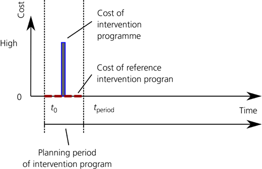
Difference in the costs related to the execution of the developed intervention programme (blue) and the reference intervention programme (red)
Difference in the costs related to the execution of the developed intervention programme (blue) and the reference intervention programme (red)
The costs of a single intervention programme consist of the intervention costs – for example, material, work labour and equipment; the user costs during the execution of the interventions – for example, costs due to longer travel time and cancelled trips; and public costs – for example, costs due to environmental impacts (Adey et al., 2020; Papathanasiou et al., 2020). The costs of the intervention programme might differ from the sum of the costs related to the individual interventions due to dependencies between the interventions leading to cost discounts. For example, executing multiple interventions together on the same link of a network disturb the traffic only once instead of once per each intervention.
Benefit quantification
Difference in the service provided
The benefit refers to the difference in the provided service of the intervention programme SIP and the reference programme Sref for all affected stakeholders (Equation 3). Figure 2 shows the evolution of the service provided by the developed intervention programme (blue solid line) and the reference programme (red dashed line) and the benefit of the intervention programme as their positive (dark grey area) and negative (light grey area) differences. The service can, for example, be measured using the travel time, where a loss in service indicates additional travel time for the user. The difference in the provided service can be quantified by quantifying the service provided of both intervention programmes using a systematic quantification method that can be found in the literature (Adey et al., 2020; Papathanasiou and Adey, 2020; Papathanasiou et al., 2020). It must be made clear that the service used to quantify the benefit of an intervention programme includes the service provided to the infrastructure owner beyond the planning period. This refers to the costs occurring for preventive interventions that are required beyond the planning period. The difference in these costs is part of the benefit of an intervention programme.
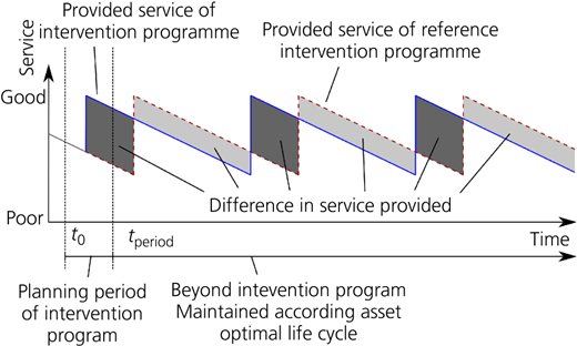
Difference in the service provided of the developed intervention programme (blue solid line) and the reference intervention programme (red dashed line)
Difference in the service provided of the developed intervention programme (blue solid line) and the reference intervention programme (red dashed line)
Figure 2 shows how an intervention programme has an impact beyond the planning period of the intervention programme. The start and end times of the planning period are indicated in Figure 2 by two dotted lines at t0 and tperiod. Since it cannot be assumed that the infrastructure is not maintained beyond the planning period, it is assumed that the infrastructure is managed in accordance with the individual optimal asset life cycles. This assumption may lead to the conclusion that the impact of the differences in the provided service occurs only for the current asset life cycles and not to future asset life cycles, as the future life cycles are only moved in time without different impacts related to the service. This, however, is valid only when no discounting is considered and when the benefit is quantified for each asset individually. With a discount rate greater than 0, which is reasonable considering uncertainties in the future regarding loads, climate change and the assets itself, the different times when future cycles begin make a difference.
The difference in service provided does include not only the service provided for the user of the infrastructure but also the difference in the service provided for the owner. The latter refers to the maintenance of the infrastructure by the owner over time and its costs. This includes all operational maintenance interventions carried out over the asset lifetime and the future rehabilitation and renewal interventions according to the optimal asset life cycle. Since the interventions included in the intervention programme change the points in time when future interventions are executed, or when the infrastructure is in a worse condition requiring more operational maintenance, the difference in these costs has to be considered in the benefit as well.
Quantification of the service over time
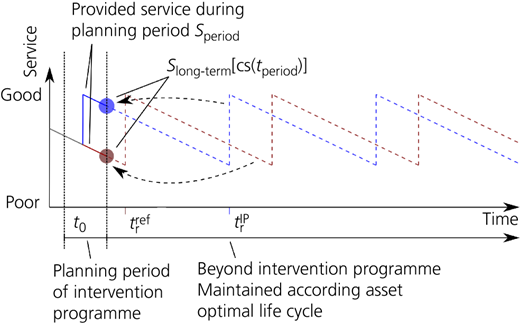
The service provided based on an intervention programme can be divided into the service provided during the planning period Speriod and the service provided beyond the end of the planning period Sbeyond (Equation 4). While the service provided during the planning period is quantified over the entire period, the service provided beyond the planning period can be quantified based on the condition of the assets at the end of the planning period, which is indicated in Figure 3 by the dots at tperiod and explained in more detail further in the text.
Principle of the service provided in respect to the intervention in the intervention programme
Principle of the service provided in respect to the intervention in the intervention programme
The service provided can best be quantified as the loss in service – that is, the inability to provide the service as intended. The quantified service provided at any given moment in time t is therefore calculated as the sum of the risks related to failures r(t) and the costs of routine maintenance cr(t) at time t. The net present value of the service provided during the planning period Speriod is equal to the discounted service provided during the planning period tperiod (Equation 5). While Equation 5 and all following equations are written in a continuous form, a discrete consideration of the risks and costs is possible by replacing the integral discounting function with a discrete summation discounting .
The service provided beyond the planning period Sbeyond is equal to the net present value of the quantified service provided in the long term Slong-term discounted over the planning period tperiod (Equation 6). The long-term service depends thereby on the optimal asset life cycle and the condition of the assets at the end of the planning period cs(tperiod). Figure 4 shows the provided service and the net present value of the long-term service provided when the specific optimal asset intervention strategy is followed over time. The curves shown represent two different starting conditions – that is, good condition for the blue curve and poor condition for the red curve.
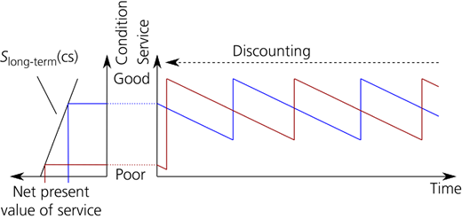
Net present value of the provided service of an intervention strategy depending on the condition of the assets at the beginning
Net present value of the provided service of an intervention strategy depending on the condition of the assets at the beginning
Equations 7–9 are used to calculate the long-term service provided as a function of the starting condition of the assets – for example, at the end of the planning period (tperiod), Slong-term[cs(tperiod)]. Equation 7 shows its division into two parts. The first summand refers to the service provided in the current life cycle (Equation 8). This requires the determination of the remaining optimal lifetime referring to the time until the asset is restored to something like new. The second summand refers to the service provided in future life cycles for an infinite time (Equation 9).
where tr refers to the time until the asset is renewed and a new life cycle begins, tcycle refers to the length of an entire life cycle, rcycle(t) refers to the risk related to failure during a life cycle and ccycle(t) refers to the costs related the execution of all interventions during a life cycle.
Example
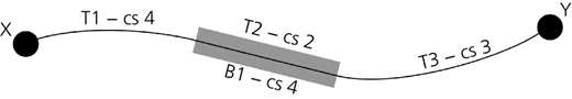
Infrastructure
The quantification of the net benefit of an intervention programme is illustrated on a realistic but fictive railway infrastructure. The railway line between stations X and Y consists of three track sections T1, T2 and T3 and one bridge B1 (Figure 5). For simplicity, the track sections are considered equal in terms of their characteristics and size. Their condition states (cs) are noted in the figure. The assumed deterioration rates are 1 cs/time unit (tu) for tracks and 0.333 cs/tu for bridges. The discount rate is 0.01. All cost values are provided in mu.
Intervention costs and risk related to failures
The impacts considered are shown in Table 3. Others can be found in the publication by Papathanasiou et al. (2020).
Impacts
| Stakeholder | Impact | Description of the impact |
|---|---|---|
| Owner | Routine interventions | Refers to the costs of executing routine interventions that are executed during the operation of the infrastructure |
| Renewal interventions | Refer to the costs of executing preventive (planned) or corrective (unplanned) renewal interventions | |
| User | Additional travel time | Impact of additional travel time on the user due to failures of the infrastructure or due to the execution of interventions |
| Accidents | Impact of accidents on the user due to failures of the infrastructure |
The costs related to the execution of planned renewal interventions consists of the costs for the execution itself and the additional travel time costs of the users (Table 4). The network-level synergies regarding the grouping of multiple renewal interventions are considered with a 30% reduction in the total costs related to the execution of interventions (Dao et al., 2019). Underlying assumptions for these reductions are the reduction in intervention costs due to economy of scale and the reduction in travel time costs due to parallel execution of interventions.
Costs related to renewal interventions in mu
| Impact | Costs related to track renewal | Costs related to bridge renewal |
|---|---|---|
| Intervention costs | 60 | 500 |
| Additional travel time costs | 40 | 100 |
| Total | 100 | 600 |
The costs for routine interventions are considered to be dependent on the condition of the assets assuming that a worse condition requires more routine interventions than an asset in something like new condition (Table 5) (Esveld, 2014).
Costs related to routine interventions in mu
| Impact | cs 1 | cs 2 | cs 3 | cs 4 | cs 5 |
|---|---|---|---|---|---|
| Routine intervention on tracks | 5 | 10 | 15 | 20 | 25 |
| Routine intervention on bridges | 0 | 15 | 30 | 45 | 60 |
To estimate the risks related to failures of the infrastructure, the probabilities of failures are multiplied by the consequence of failures (Papathanasiou et al., 2016). The consequences consist of the corrective renewal intervention, the additional travel time for the users due to longer travel times and accidents (Table 6). The probabilities of a track and bridge failure are dependent on the condition of the assets. The consequences of a track failure assume that the corrective renewal intervention costs the same as a planned renewal. The duration of the occurrence, however, is longer due to the reaction time between a failure occurrence and the start of the renewal intervention, and therefore, the costs of additional travel time are higher. The accident costs are assumed even higher. The same assumptions are made for the consequences of a bridge failure. Here, the consequences of an accident are much higher than for the track based on the assumption that an accident of a train on a bridge leads to much more injuries and fatalities than an accident on the open track.
Risk estimation related to failures dependent on condition states (cs)
| Value | Track | Bridge | ||||||||
|---|---|---|---|---|---|---|---|---|---|---|
| cs 1 | cs 2 | cs 3 | cs 4 | cs 5 | cs 1 | cs 2 | cs 3 | cs 4 | cs 5 | |
| Probability | 0.01 | 0.02 | 0.03 | 0.04 | 0.05 | 0.001 | 0.002 | 0.004 | 0.008 | 0.016 |
| Risk: mu | 10 | 20 | 30 | 40 | 50 | 10 | 20 | 40 | 80 | 160 |
| Intervention costs: mu | 60 | 500 | ||||||||
| Additional travel time costs: mu | 140 | 1000 | ||||||||
| Accident costs: mu | 800 | 8500 | ||||||||
| Total consequences: mu | 1000 | 10 000 | ||||||||
Individual optimal asset life cycles
Based on the impacts and interventions considered, the strategy related to the optimal life cycles of each individual asset is estimated. Therefore, the condition states are determined when interventions should be executed to minimise the life-cycle costs considering the defined deterioration rates and cost values for the different impacts. With the given values, renewal interventions should be executed when the assets are in condition state 4 for both tracks and bridges. The renewal interventions are assumed to be perfectly effective – that is, they bring the condition of the assets back to state 1.
The method for the quantification of the net benefit of an intervention programme considers the assets to be managed beyond the planning period according to their optimal asset life cycles. This requires the estimation of the net present value of the long-term service provided S long-term(cs) dependent on the starting condition (cs). Table 7 shows the total net present value of the service provided (Equation 7), the risks and costs during the time until the asset is at the beginning of a new life cycle (Equation 8) and the risks and costs for the consideration of an infinite number of life cycles afterwards (Equation 9).
Net present values of the long-term service provided depending on the starting condition (Equation 7)
| Asset type | cs | Risks in remaining cycle | Costs in remaining cycle | Strategy long-term risks | Strategy long-term costs | Total S long-term(cs) |
|---|---|---|---|---|---|---|
| Track | 1 | 97 | 145 | 2390 | 3562 | 6194 |
| 2 | 88 | 141 | 2414 | 3598 | 6241 | |
| 3 | 69 | 132 | 2439 | 3634 | 6274 | |
| 4 | 40 | 119 | 2463 | 3670 | 6291 | |
| 5 | 50 | 124 | 2463 | 3670 | 6306 | |
| Bridge | 1 | 264 | 738 | 2527 | 7050 | 10 685 |
| 2 | 257 | 745 | 2553 | 7120 | 10 964 | |
| 3 | 250 | 747 | 2578 | 7191 | 11 176 | |
| 4 | 243 | 745 | 2604 | 7263 | 11 290 | |
| 5 | 226 | 738 | 2630 | 7336 | 11 383 |
Equations 10–13 show the exemplary calculation for a track in condition state 3. Applying the strategy defined, the track deteriorates first for 2 tu to condition state 4 before it is renewed and brought back to condition state 1. The risks in the remaining cycle consists therefore of the risks in condition states 3 and 4 discounted by 1 and 2 tu, which equals 69 mu (Equation 10). The costs for the remaining cycle are estimated in equal way (Equation 11). The long-term strategy risks (Equation 12) and costs (Equation 13) are calculated by estimating the risk and cost values for a single cycle – that is, once from conditions 1 to 4 within 4 tu; discounting them for an infinite number of cycles – that is, equal to factor 1/0.039; and considering the remaining cycle time of 3 tu – that is, factor 1/1.03.
Reference intervention programme
The reference intervention programme consists of the interventions according to the individual asset life cycles meaning that all assets with condition state 4 have a renewal intervention. This results in a reference intervention programme consisting of a renewal on track section T1 and a renewal of bridge B1. Table 8 shows the reference intervention programme with the intervention costs – that is, a total of 700 mu – and the impacts related to the service provided – that is, a total of 29 501 mu.
Reference intervention programme
| Asset | Current condition | Intervention | Costs | Service during the planning period | Condition after the planning period | Long-term service dependent on condition | Total service |
|---|---|---|---|---|---|---|---|
| S period | cs(t period) | S beyond(cs) | S | ||||
| T1 | 4 | Renewal | 100 | 15 | 2 | 6179 | 6194 |
| T2 | 2 | None | 0 | 30 | 3 | 6211 | 6241 |
| T3 | 3 | None | 0 | 45 | 4 | 6229 | 6274 |
| B1 | 4 | Renewal | 600 | 10 | 2 | 10 782 | 10 792 |
| Total | 700 | 100 | — | 29 401 | 29 501 |
As an example, the calculation for executing a renewal on track T1 is shown in Equations 14 and 15. Executing the renewal intervention on track T1, which is currently in condition 4, costs 100 mu, consisting of 60 mu of intervention costs and 40 mu of additional travel time costs during the execution of the intervention. It is assumed here that the intervention is executed at the beginning of the planning period, and therefore, the impacts on the service provided during the planning period is estimated in respect to the restored condition state 1 – that is, 15 mu (Equation 14). During the 1 tu planning period, the risks related to failures and the costs of routine maintenance of a track in condition state 1 are considered. The asset deteriorates for 1 tu until the planning period is over. Considering the deterioration rate for tracks of 1 cs/tu, the condition after the planning period is 2. Table 7 provides the net present value of the long-term service provided depending on condition state 2 – that is, 6241 mu for a track in condition state 2. This is discounted by the planning period in order to estimate the net present value of the service provided beyond the planning period (Equation 15). Combining the 15 mu of the service related to the period and the 6179 mu related to the long-term service equals the total service provided – that is, 6194 mu.
Net benefit
To illustrate the quantification of the net benefit of intervention programmes given the network-level synergies and constraints, the net benefit of two candidate intervention programmes is quantified. Different from the reference intervention programme based on the individual optimal life cycles for each asset, the candidate intervention programmes consider the reduction in intervention costs when track interventions are combined and that a renewal of bridge B1 requires track T2 to be renewed as well, as they are structurally dependent. The second intervention programme also considers a budget limitation of 600 mu.
The intervention programmes without and with the consideration of a budget limitation are shown in Tables 9 and 10, respectively. The tables list the costs and the impacts related to the service provided, which are further considered in Table 11 to estimate the net benefit of the two intervention programmes. The intervention programme without a budget limitation consists of a renewal on each asset, while the intervention programme considering a budget limitation consists only of a renewal intervention on track sections T1 and T3.
Intervention programme without a budget limitation
| Asset | Current condition | Intervention | Costs | Service loss during the planning period | Condition after the planning period | Long-term service loss dependent on condition | Total service |
|---|---|---|---|---|---|---|---|
| S period | cs(t period) | S beyond(cs) | S | ||||
| T1 | 4 | Renewal | 70 | 15 | 2 | 6179 | 6194 |
| T2 | 2 | Renewal | 70 | 15 | 2 | 6179 | 6194 |
| T3 | 3 | Renewal | 70 | 15 | 2 | 6179 | 6194 |
| B1 | 4 | Renewal | 600 | 10 | 2 | 10 782 | 10 792 |
| Total | 810 | 55 | — | 29 319 | 29 374 |
Intervention programme with a budget limitation of 600 mu
| Asset | Current condition | Intervention | Costs | Service loss during the planning period | Condition after the planning period | Long-term service loss dependent on condition | Total service |
|---|---|---|---|---|---|---|---|
| C | S period | cs(t period) | S beyond(cs) | S | |||
| T1 | 4 | Renewal | 70 | 15 | 2 | 6179 | 6194 |
| T2 | 2 | None | 0 | 30 | 3 | 6211 | 6241 |
| T3 | 3 | Renewal | 70 | 15 | 2 | 6179 | 6194 |
| B1 | 4 | None | 0 | 124 | 4 | 11 295 | 11 419 |
| Total | 140 | 184 | — | 29 864 | 30 048 |
Quantification of the net benefit of the intervention programmes
| Cost value | Formulation | Intervention programme without a budget limitation | Intervention programme with a budget limitation of 600 mu |
|---|---|---|---|
| Costs of the intervention programme | C IP | 810 | 140 |
| Costs of the reference intervention programme | C ref | 700 | 700 |
| Difference in costs | ΔC = C IP − C ref | 110 | −560 |
| Service loss provided by the intervention programme | S IP | −29 374 | −30 048 |
| Service loss provided by the reference intervention programme | S ref | −29 501 | −29 501 |
| Difference in service provided | B = ΔS = S IP − S ref | 127 | −547 |
| Net benefit | NB = ΔS − ΔC | 17 | 13 |
Figures 6 and 7 show graphically the quantification of the net benefit. The graphs on the left show the differences in costs and in the service provided, as well as the net benefit of the intervention programmes compared with the reference programme. A negative cost in the case of no budget limitation means that the intervention programme leads to higher intervention costs during the planning period compared with the reference programme – that is, less net benefits. The positive difference in the service provided means that the interventions lead to less impacts in the future. Its quantification is shown in the right graph for the first 50 years. It has to be noted, though, that the quantification of the loss in service considers an infinite horizon. The discounted risk, maintenance and renewal costs are considered as they are expected when the assets are managed according to the individual asset life cycles beyond the planning period – that is, from year 2 on ward.
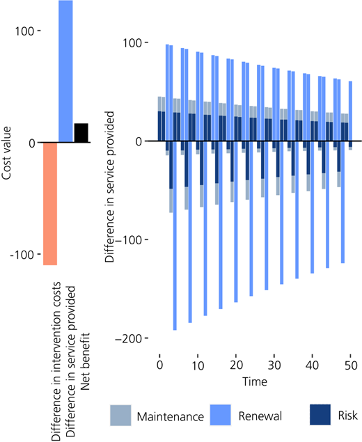
Quantification of the net benefit (left) and the difference in service provided over time (right) for the intervention programme without a budget limitation
Quantification of the net benefit (left) and the difference in service provided over time (right) for the intervention programme without a budget limitation
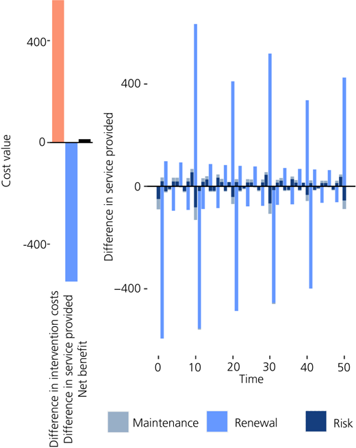
Quantification of the net benefit (left) and the difference in service provided over time (right) for the intervention programme with a budget limitation of 600 mu
Quantification of the net benefit (left) and the difference in service provided over time (right) for the intervention programme with a budget limitation of 600 mu
As an example, the intervention programme without the consideration of a budget limitation includes renewal interventions on all four assets. The costs sum up to 810 mu, consisting of 600 mu for the renewal of bridge B1 and 210 mu for the sum of the three track renewals. The track renewals make use of the synergies between the interventions reducing the costs by 30% – that is, 100 mu × 3 × (1 − 0.3) = 210. The impacts on the service provided are quantified based on the asset condition and sum up to 29 374 mu. The difference in costs – that is, 110 mu – and the difference in the service provided – that is, 127 – result in a net benefit of 17 mu (Table 11).
Discussion
The example shows how the net benefit of an intervention programme can be quantified based on a reference intervention programme that is based on the optimal life cycles of the individual assets. Thereby, the net benefit of an intervention programme considers the costs related to the execution of interventions for all relevant stakeholders – that is, owner and user – and the impacts on the service provided to the different stakeholders during and beyond the planning period. In the example, both developed intervention programmes have a positive net benefit, indicating that they are beneficial compared with the reference intervention programme. The intervention programme developed without a budget limitation, for example, has 110 mu higher costs related to the execution of the intervention programme, while the loss in the service provided to the owner and user is 127 mu less than the reference intervention programme.
Further, the systematic quantification allows comparison of different intervention programmes. For example, comparison of the developed intervention programmes indicates that the additional costs of 670 mu of the intervention programme without a budget limitation compared with the intervention programme with a budget limitation increase the net benefit by 4 mu. Therefore, the quantification makes it possible to decide clearly whether interventions are beneficial when executed in an earlier state than defined by the individual asset life cycle. For example, bringing the renewal of track T3 forward increases the net benefit due to the possible cost reductions due to the network-level synergies. The quantification also allows the identification of the interventions that can be postponed with the least loss in net benefit when network-level constraints restrict the execution of all interventions. In the example, the renewal of bridge B1 is postponed in the situation with a limited budget because this reduces the net benefit less than postponing another intervention.
The example shows the usefulness of quantifying the condition-dependent net present value of the impacts incurred when managing an asset according to its individual optimal life cycle (Table 7). This enables the consideration of the benefit beyond the planning period – that is, long-term benefit – based on the asset condition at the end of the planning period. Through the values used in the example, the importance of considering the long-term benefit correctly can be seen. For example, for the intervention programme developed with a budget limitation, the major part of the difference in the service provided – that is, −547 mu – is due to the difference in the service provided beyond the planning period – that is, −463 mu. This means that in this situation, 84% of the benefit occurs beyond the planning period.
The example shows how intervention programmes for infrastructure networks with different asset types – for example, tracks with shorter lifetimes and bridges with longer lifetimes – can be valued using net benefit quantification while considering the individual optimal life cycles of the assets and the network-level effects. This net benefit quantification can be used in optimisation models to determine the intervention programme with the highest net benefit. It allows including all relevant considerations within a single objective function that ensures the comparability of different candidate interventions. Overall, the net benefit quantification, the consistent consideration of the impacts of interventions over time and the possibility to be used to develop optimal intervention programme is an improvement to the methods and models used in practise and research that all lack in one or more of these considerations.
Conclusion
The method presented in this paper can be used to quantify the net benefit of intervention programmes, which in turn can be used in the determination of the optimal intervention programme. The net benefit of an intervention programme thereby quantifies the difference in the service provided and the costs related to the execution of the interventions comparing a candidate intervention programme with a reference intervention programme. The method, different from the methods used in existing asset-management systems, considers the benefit in the long term – that is, beyond the planning period – by considering the service provided by the assets when they are managed according to their individual optimal life cycles in the time beyond the intervention programme. This consistent consideration and quantification of the long-term impacts of interventions allows the quantification of the net benefit of intervention programmes on entire infrastructure networks composed of different asset types with widely varying life cycles.
The method supports decision-makers when deciding whether interventions should be executed earlier or later than the individual optimal point in time of the asset due to network-level effects – that is, synergies between interventions on different assets and network-level constraints limiting the execution of different interventions. This possibility enables the improvement of existing management systems for and research studies on determining optimal intervention programmes, which are most often limited in the consideration of network-level effects.
In conclusion, this method helps pave the way for the use of sophisticated operational research methods for the automated determination of optimal intervention programmes in infrastructure-management systems – that is, a step towards exploiting the benefits of digitalisation.


Acknowledgement
The work presented here has received funding from Horizon 2020, the EU’s Framework Programme for Research and Innovation, under grant agreement number 769373.
