


Road infrastructure asset management requires making decisions that affect how infrastructure provides service – for example, the intervention strategies to follow for specific assets, the intervention programmes to implement for entire networks and the way for interventions to be executed once it is decided that they should be executed. These decisions should be made to maximise the net benefit of infrastructure for all stakeholders and be made consistently and transparently. Currently, the definitions of service used by road infrastructure asset managers either are incomplete or are built on combinations of metrics, which give an idea of service but do not measure service directly. Neither allows for consistent and transparent decision-making that leads to the maximisation of the net benefit for all stakeholders. In this paper, a definition of the service provided by road infrastructure is provided that enables consistent and transparent decisions to maximise the net benefit for all road infrastructure stakeholders. The service definition is used to determine the net-benefit-maximising intervention strategy that shows its usefulness and its ability to let stakeholders see how they will be affected by decisions and that all of their concerns have been adequately taken into consideration when decisions are made.
Notation
- Co
overall cost of object o
cost of object o in year t
cost of impact I on object o in year t
cost of impact I on object o in year t related to state s
duration of intervention i on object o
- fI-i(s)
factor of impact I related to intervention i executed in state s according to the strategy
- fI-s
factor of impact I related to state s
- lo
length of object o
probability of an accident on object o
transition probability of an object to change its state from i to j in year t
probability of object o to be in state s in year t
- qo
traffic flow on object o
- ucI
unit cost of impact I
unit duration of intervention i
unit quantity of impact I on object o
- vo
traffic speed on object o
Introduction
Roads are built and maintained to provide a service – for example, the ability to transport persons and goods from A to B in a specific amount of time, with a relatively low probability of the goods being damaged and the persons being hurt or losing their lives. As roads deteriorate over time, interventions need to be executed to ensure that the provided service stays within acceptable bounds and, if it is not within acceptable bounds, to restore it so that it is once again within acceptable bounds. In an effort to do this, road managers regularly make decisions that affect how their infrastructure provides service. For example, they determine the optimal intervention strategies for specific assets, the optimal intervention programmes for entire networks and the optimal way for interventions to be conducted once it is decided that they should be executed. In order to make these decisions consistently and transparently, it is imperative to have a complete definition of the service provided by the infrastructure. Although many current explicit and implicit definitions of service exist, they are often incomplete.
Examples of current definitions of service can be grouped as explicit definitions, where efforts are made to measure service directly, and implicit definitions, where efforts are made to measure service indirectly. An example of a very simple, but often used, explicit hierarchy would be to take into consideration only the impact on the owner in terms of intervention costs, something which is done in the base analysis of many infrastructure management systems (Astra, 2010; FHWA, 2002). Some examples of more complete explicit hierarchies are ones that are used on the project level, which include the impact hierarchy developed by the New Zealand Transport Agency (NZTA, 2010) to evaluate all road project submissions and the impact hierarchy developed by Ecoplan (2010) to be used by the Swiss road authority to evaluate road projects. Many, if not all, of these hierarchies, however, neglect numerous impact types, which makes it impossible to use them to make net-benefit-maximising decisions pertaining to infrastructure. For example, if only intervention costs are considered, then the decision maker is implicitly assuming that none of the other impacts, such as accident, travel time, vehicle operation, comfort and noise, matters. If the hierarchy proposed by the NZTA (2010) is used, then impacts such as comfort, noise and particle emissions and socio-economic activity are assumed to not matter. As a public road has many different stakeholders with different views of what is important, hierarchies determined through stakeholder surveys are also often not orthogonal – for example, access and travel time (Kumares and Labi, 2007).
Examples of implicit hierarchies are ones that have been developed using metrics such as those proposed by Abbott et al. (1998), Baird and Stammer (2000), the Organisation for Economic Co-operation and Development (OECD, 2001), the Federal Highway Administration (FHWA, 1996), the World Bank (2003), Kassoff (2001), Bai et al. (2011) and Patidar et al. (2007). When metrics, such as average speeds weighted by person-kilometres, average delays, average travel time, average trip time and manoeuvrability measured by vehicles per hour per lane (Abbott et al., 1998), are used, one obtains an idea that the measure of travel time is important, but, as many aspects of travel time are used in the metric and different weights are assigned to these, there is no clear view of what the service provided is and, therefore, no clear way to make decisions that maximise the net benefit. This, of course, is not to say that metrics are not important or useful. They are very important in having an understanding in how the transport system provides an adequate level of service and is very useful in communicating decisions to stakeholders but is just not directly useful in determining which decisions are optimal.
In order to eliminate the confusion that often results from explicit but incomplete and non-orthogonal lists and from the use of metrics instead of service, an impact hierarchy is proposed in this paper that can be used to take into consideration most, if not all, of the relevant impacts to the ‘principal’ stakeholders of public road infrastructure – that is, those whose positive impacts should be maximised. In other words, the net negative impact should be minimised. It is considered that each person at a point in time can be classified into one of four stakeholder groups: the owner, the users, the directly affected public and the indirectly affected public. The impact types in the hierarchy are given to a level of detail in which they could reasonably be quantified. To help ensure orthogonality and give an idea of how the impact is to be quantified, a pillar of sustainability – that is, the economic, environmental or social pillar – is associated with each of the lowest-level impacts. An example of each impact type, as well as at least one example in literature of how the impact can be quantified, is given.
This impact hierarchy is for existing public roads, which are to be managed to minimise the net negative impact that society as a whole obtains from the infrastructure. Only changes that are relevant to society as a whole are, therefore, considered – that is, positive impacts on one stakeholder that are negative impacts on another are not taken into consideration. For example, the income that is received from charging a toll on public road is not considered, as it is a positive impact on the owner but a negative impact of equal magnitude on the users. In order to demonstrate how the impact hierarchy could be used, it is used in the determination of the optimal intervention strategy for a fictive road section, composed of multiple objects. The work presented here builds on that done by Adey et al. (2010, 2012, 2018).
Stakeholders
A stakeholder is herein considered as an individual, group or organisation which is affected by changes to public roads. Being a stakeholder is time dependent – that is, when a person is driving a vehicle on a road, they are a user at that point in time. When the person is off the road and in their house far from the road, they are part of the indirectly affected public. It is considered that all stakeholders can be grouped as either first-level or second-level stakeholders. The first-level stakeholders are those whose net positive impacts should be maximised. The second-level stakeholders are those whose impacts are the outcome of the maximisation of the net impacts of the first-level stakeholders and should be monitored.
The four first-level stakeholder groups are the owner, the users, the directly affected public and the indirectly affected public. It is assumed that all impacts to be maximised can be attributed to one of these four principal stakeholder groups. The impacts are attributed to the stakeholder who is most directly affected. The definitions of each principal stakeholder group are given in Table 1.
Principal stakeholder groups
| Stakeholder group | Definition |
|---|---|
| Owners | Persons who pay for the interventions on the infrastructure |
| Users | Persons who are using the roads |
| Directly affected public | Persons who are in the vicinity of the road but are not using it |
| Indirectly affected public | Persons who are not in the vicinity of the road but are affected by its use |
Second-level stakeholder groups, such as operators, contractors, environmental protection groups and financial institutions, are not considered further than they are considered when considered as one of the aforementioned stakeholders. The impacts on these stakeholder groups are only the outcome of efforts to maximise the positive net impact of the four first-level stakeholders. It is noted that, in specific situations, one might be interested in maximising the net benefit for a subgroup of stakeholders, which may consist of stakeholders from the first and/or the second level. If this is the case, then each stakeholder group to be considered needs to be defined.
Impacts
The impacts on each stakeholder group are grouped as impact types. The impact types are subdivided at increasingly fine levels until the impact of each type can be reasonably and objectively quantified. To help ensure orthogonality in the impact hierarchy, each impact type, on the lowest defined level, is explained and classified as contributing to one of the pillars of sustainability (i.e. economic, societal, environmental). An example is given for each to help clarify its meaning, and an example in the literature of how it has been quantified by others is given. The impact hierarchy is given in the tables in the following subsections.
Owner
The impacts attributed to the owner are grouped as intervention costs (Table 2) – that is, the impact on the owner of maintaining the expected level of service or, in other words, the cost of executing of interventions. The impact indicators are the amount of labour, equipment and material to be used to execute interventions – for example, intervention w required x man-hours, y generator-hours and z kilograms of material. The monetary value placed on (a) the labour used represents the economic impact of persons performing tasks – that is, the value from society’s perspective of the person executing the intervention; (b) the material used represents the economic impact of people ensuring that materials are available for use – that is, the value from society’s perspective of persons preparing the materials for use; and (c) the equipment used represents the economic impact of people ensuring that equipment is available for use – that is, the value from society’s perspective of persons preparing the equipment for use. The estimation of the value of an intervention is often done using one of two approaches.
A disaggregate approach is where expenditures for each item or activity are estimated and summed. When this approach is used the work break down structure of the intervention project it is often used.
An aggregate approach is where the sum of all expenditures is estimated directly. An aggregate approach often includes regression analysis and historical information.
Owner impact types
| Level 1 | Level 2 | Example in literature | ||
|---|---|---|---|---|
| Label | Description | Label | Description | |
| Intervention | Impact of executing interventions | Labour | Economic impact of people performing tasks | Adey et al. (2017) |
| Material | Economic impact of people ensuring that materials are available for use | |||
| Equipment | Economic impact of people ensuring that equipment is available for use | |||
Users
During the interventions, users experience inconveniences such as traffic jams and having to take detours. These inconveniences can be quantified in terms of negative impacts – for example, the higher probabilities of accidents, increased physical exhaustion, increased travel times and increased fuel consumption and vehicle maintenance costs. In between interventions, deterioration processes result in a worsening condition of infrastructure objects, which results in changes in how stakeholders are affected – for example, increases in the number of accidents, increases in travel time and increased vehicle maintenance costs. The impacts attributed to the users are grouped as shown in Table 3.
Users impact types
| Level 1 | Level 2 | Examples in literature | ||
|---|---|---|---|---|
| Label | Description | Label | Description | |
| Accident | Impact on the users due to the users being involved in an accident | Property damage | Economic impact of repairing the vehicle | Kasnatscheew et al. (2016) |
| Injury | Societal impact due to the injury | |||
| Fatality | Societal impact due to fatality | |||
| Travel time | Impact of travel condition in terms of time lost | Work | Economic impact of wasting work time travelling | de Palma (2011) |
| Leisure | Economic impact of wasting leisure time travelling | |||
| Vehicle operation | Impact of travel condition on the vehicle cost | Operation | Economic impact of people ensuring that fuel and oil is available for use | Maibach et al. (2006) |
| Maintenance | Economic impact of people repairing vehicles and ensuring that materials, for example, tyres and brake pads, are available for use | |||
| Comfort | Impact of travelling on the users | Physical | Societal impact of obtaining, for example, bruises from an extremely bumpy ride | Gilchrist and Allouche (2005) |
| Psychological | Societal impact of having, for example, anxiety due to a perceived increase in the probability of being involved in an accident or of seeing things while travelling | |||
| Noise | Societal impact due to the users coming in contract with sound emissions | Dykes (2018) | ||
Accident
Accidents result in damage to the property of involved parties. Although the owners will often repair the damaged infrastructure following an accident, the users will be required to repair their vehicles. The users will also be affected by any injury and, of course, fatality that may befall them. The accident impact type attributed to the users is subdivided into property damage, injury and fatality impact types.
The property damage impact type represents the economic impact of repairing the vehicle – that is, of providing the users with a functioning mode of transport similar to the one being used before the accident – for example, the costs of the labour, materials and equipment required to replace the bumper on a vehicle that has been in an accident. The value of this impact type can be approximated using the receipts from past repairs.
The injury and fatality impact types attributed to the users represent the social impact due to injuries and fatalities, respectively. They represent the change in interactions between persons that will occur because the user is injured or has lost their life. It is not to be confused with the injury impact type and the fatality impact type attributed to the directly affected public (see the section headed ‘Directly affected public’) or to the indirectly affected public (see the section headed ‘Indirectly affected public’). The value of these impact types can be estimated by using the users’ willingness to pay to avoid injury or fatality.
Travel time
The amount of time travelling on the road is a function of the speed driven and the distance travelled. It is affected by many factors, such as road condition (drivers feel comfortable on a smooth road and therefore drive faster than on a bumpy road), the daily traffic volume in relation to the road capacity, road geometry, whether or not an intervention is being executed and whether or not a detour is required. The economic impact of wasting work and leisure time travelling may be thought of as the loss of productivity of the users due to time spent travelling. The value of travel time can be determined using willingness to pay surveys.
Vehicle operation
The vehicle operation impact type represents the economic impact of ensuring that fuel and oil is available for use and the economic impact of repairing vehicles and ensuring that materials – for example, tyres and brake pads – are available for use. The value of the vehicle operation impact type can be approximated using the receipts from fuel and vehicle service receipts.
Comfort
The comfort impact type is subdivided into the physical and psychological impact types. The physical impact type represents the social impact of obtaining, for example, bruises from an extremely bumpy ride. It represents the change in interactions between people that will occur because the physical change in the users due to the bumpy ride. The psychological impact type represents the impact of having, for example, anxiety due to a perceived increase in the probability of being involved in an accident or of seeing things while travelling – for example, aesthetics. It is likely that any economic impacts relevant to society due to the physical and psychological impacts of travelling, such as the loss of productivity, are negligible in developed countries. The value of degrees of bumpiness could be determined through willingness-to-pay investigations.
Noise
The noise impact type represents the social impact due to the users coming in contact with sound emissions. It captures the changes that occur in the interactions between people due to sound emissions – for example, the difficulty of communication between the driver and passenger during driving. The value of an amount of sound emissions can be determined through willingness-to-pay investigations.
Directly affected public
The impacts attributed to the directly affected public are grouped in the same way as the impacts attributed to the users (Table 4). The reason that they are handled separately is that the directly affected public is affected in ways fundamentally different from the users.
Directly affected public impact types
| Level 1 | Level 2 | Examples in literature | ||
|---|---|---|---|---|
| Label | Description | Label | Description | |
| Accidents | Impact on the directly affected public due to being involved in an accident | Property damage | Economic impact of repairing property damaged due to a vehicle coming off the road | Kasnatscheew et al. (2016) |
| Injury | Societal impact due to the injury | |||
| Fatality | Societal impact due to fatalities | |||
| Comfort | Impact of travelling on the directly affected public | Physical | Societal impact of physical changes due to people travelling on the road, for example, due to vibrations | Gilchrist and Allouche (2005) |
| Psychological | Societal impact of having, for example, anxiety due to a perceived increase in the probability of being involved in an accident, due to others travelling | |||
| Noise | Societal impact due to the directly affected public coming in contract with sound emissions | Korzhenevych et al. (2014) | ||
| Particle emissions | Impact on people due to the environment being impacted by particle emissions | Carbon dioxide | Societal impact due to emissions (human health) | Korzhenevych et al. (2014) |
| PM10 Nitrogen monoxide Carbon monoxide Aldehydes Nitrogen dioxide Sulfur dioxide Polycyclic aromatic hydrocarbons Dust | Same as for carbon dioxide | Jensen et al. (2004) | ||
Accident
The accident impact type is subdivided into property damage, injury and fatality impact types. The property damage impact type represents the economic impact of repairing damaged property to the condition it was in prior to the occurrence of the accident – for example, the costs of the labour and materials required to repair a retaining wall that has been damaged in an accident. The value of this impact type can be approximated using the receipts from past repairs.
The injury impact type and the fatality impact type attributed to the directly affected public represent the societal impact due to injuries and fatalities, respectively. They represent the change in interactions between persons that will occur because someone other than the users is injured or dead. It is not to be confused with the injury impact type and the fatality impact type attributed to the indirectly affected public. The value of these impact types can be estimated by using willingness to pay of the directly affected public to avoid injury or fatality.
Comfort
The comfort impact type is subdivided into the physical and psychological impact types. The physical impact type represents the societal impact of obtaining, for example, discomfort through vibrations that occur due to road use. It represents the change in interactions between people that will occur because of the physical change in the directly affected public. The psychological impact type represents the social impact of having, for example, anxiety due to a perceived increase in the probability of being involved in an accident or of seeing the infrastructure – for example, aesthetics. It is believed that any economic impacts to be attributed to the directly affected public due to the physical and psychological impacts of others travelling, such as the loss of productivity, are negligible. The value of degrees of bumpiness can be determined through willingness-to-pay investigations.
Noise and particle emissions
The noise and particle emission impact type represents the social impact due to the directly affected public coming into contact with sound and particle emissions. The sound emission impact type captures the changes that occur in the interactions between people due to sound emissions – for example, the necessity to change where people meet due to excess noise. The value of an amount of sound emissions can be determined through willingness-to-pay investigations.
The particle emission impact type represents the societal impact due to emissions emitted during the production and transport of materials and persons and that directly affect persons. It is meant to capture the changes that occur in the interactions between people due to changes in the people – for example, due to sickness. It is subdivided according to the particles emitted – for example, carbon dioxide (CO2), particulate matter (PM10), nitrogen monoxide (NO), carbon monoxide (CO), aldehydes, nitrogen dioxide (NO2), sulfur dioxide (SO2), polycyclic aromatic hydrocarbons and dust. The value of each amount can be determined by analysing historical records or by conducting empirical studies using emission measurement tools and instruments.
Indirectly affected public
The indirectly affected public are those that are affected by roads through other mediums – for example, a person who is affected by an increase in the temperature of the earth due to the carbon dioxide emitted during the execution of an intervention on a road. The impacts attributed to the indirectly affected public are grouped as safety, socio-economic activity, particle emissions and environment consumption. Tables 5 and 6 list the most common impact types and indicators. It is noted that several impact types, such as gas and particle emission, also directly affect the users and the directly affected public. It is assumed, however, that these impacts are minimal.
Indirectly affected public impact types (1/2)
| Level 1 | Level 2 | Level 3 | Examples in literature | |||
|---|---|---|---|---|---|---|
| Label | Description | Label | Description | Label | Description | |
| Accidents | Impact on the indirectly affected public of accidents occurring on roads | Injuries | Economic impact due to an injury | Kasnatscheew et al. (2016) | ||
| Fatalities | Economic impact due to a fatality | |||||
| Socio-economic activity | Contribution of the road operation to socio-economic development | Persons | Impact of not being able to transport people | Productiveness | Economic impact due to not being able to travel (e.g. not being able to work) | Gilchrist and Allouche (2005) |
| Health | Societal impact due to injuries and fatalities of not being able to get proper medical care | |||||
| Goods | Impact of not being able to move goods | Productiveness | Economic impact due to not being able to deliver goods (e.g. because of not being able to work as planned) | Gilchrist and Allouche (2005) | ||
| Health | Societal impact due to not being able to deliver goods (e.g. due to fatalities because of lack of food or medical supplies) | |||||
| Employment | Impact of interventions in terms of employing people | Gilchrist and Allouche (2005) | ||||
Indirectly affected public impact types (2/2)
| Level 1 | Level 2 | Level 3 | Examples in literature | |||
|---|---|---|---|---|---|---|
| Label | Description | Label | Description | Label | Description | |
| Particle emissions | Impact on people due to the environment being impacted by particle emissions | Carbon dioxide | Impact due to the emissions | Production | Environmental impact of emissions emitted during the production of materials | Korzhenevych et al. (2014) |
| Material transport | Environmental impact of emissions emitted during the transport of materials | |||||
| Person transport | Environmental impact of emissions emitted during travel | |||||
| Health | Societal impact due to emissions (human health) | |||||
| PM10 Nitrogen monoxide Carbon monoxide Aldehydes Nitrogen dioxide Sulfur dioxide Polycyclic aromatic hydrocarbons Dust | Same as for carbon dioxide | Jensen et al. (2004) | ||||
| Environment consumption | Depletion of finite amounts of non-renewable resources | Energy | Environmental impact due to the consumption of energy not related to emissions (e.g. depletion of finite amounts of non-renewable energy sources) | Pullen (2000), Robinette and Epps (2010) | ||
| Materials | Environmental impact of consumption of materials not related to emissions | |||||
| Land | Environmental impact due to the consumption of land not related to emissions | |||||
| Culture | Societal impact of changing things important to society’s identity (of which heritage is part) | |||||
Accident
The injury and fatality impact types attributed to the indirectly affected people represent the economic impact due to injuries and fatalities. They represent the loss in productivity due to injuries and fatalities. It includes changes to human activity, such as a doctor’s time in an emergency room and the time required to ensure that an insurance company conducts the required financial transactions. The impact indicator is the amount of work time lost compared with the reference case where the accident had not occurred. The value of each amount can be determined by estimating the loss of productivity of the person involved in the accident.
Socio-economic activity
The socio-economic activity impact type represents the contribution of the road to socio-economic development. It is composed of persons, goods and employment impact types.
The person impact type is further divided into productiveness impact type and health impact type. The productiveness impact type represents the economic impact due to not being able to travel – for example, a farmer cannot harvest their entire crop because they need to spend a significantly larger portion of their time getting their goods to market. The value of each amount can be determined by conducting simulations of the performance of the region. The health impact type represents the societal impact due to injuries and fatalities that occur due to not being able to obtain standard medical care, due to a shortage of available persons. The value of each amount can be determined by conducting simulations of the region.
The goods impact type is also further divided into productiveness impact type and health impact type. The productiveness impact type represents the economic impact due to not being able to deliver goods – for example, a farmer cannot plant their crop on time since fertilisers could not be delivered as planned. The health impact type represents the societal impact due to injuries and fatalities due to goods such as food or medical supplies not being delivered as planned. This includes, for example, the change in society that occurs due to the fatality of someone in a hospital who would not have died if medical supplies have been delivered as planned.
The employment impact type represents the societal impact of executing interventions in terms of employing people that is not captured by the impact type attributed to the owner due to the execution of interventions or the users due to the maintenance of vehicles used for travelling. It includes economic development. The impact indicator is the amount of work provided. The value can be estimated using economic impact assessment models, using predictions of business output, value added, employment level, wages and salaries, and wealth made.
Emissions
The emission impact type of the indirectly affected public represents the environmental and societal impacts due to emissions emitted during the production and transport of materials and persons. It is subdivided according to the particles emitted – for example, carbon dioxide, PM10, nitrogen monoxide, carbon monoxide, aldehydes, nitrogen dioxide, sulfur dioxide, polycyclic aromatic hydrocarbons and dust. Each of these is further subdivided into (a) the production impact type, which represents the environmental impact of emissions emitted during the production of materials; (b) the material transport impact type, which represents the environmental impact of emissions emitted during the transport of materials to and from the construction site; (c) the person transport impact type, which represents the environmental impact of emissions emitted during travel; and (d) the health transport impact type, which is societal impact due to emissions (human health). It is meant to capture the changes that occur in the interactions between people due the changes in the people – for example, due to sickness. Their value can be determined by analysing historical records or by conducting empirical studies using emission measurement tools and instruments.
Environment consumption
The environment consumption impact type represents the depletion of finite amounts of non-renewable resources. It is subdivided into the energy impact type, the material impact type, the land impact type and the culture impact type. The energy impact type represents the environmental impact due to the consumption of energy not related to emissions – for example, depletion of finite amounts of non-renewable energy sources. The material impact type represents the environmental impact of consumption of materials not related to emissions – for example, the consumption of wood has an impact on woodland areas. The land impact type represents the environmental impact due to the consumption of land not related to emissions – for example, increased environmental damages due to floods. The culture impact type represents the societal impact of changing things important to society’s identity (of which heritage is part). The value can be estimated through willingness-to-pay investigations.
Example
Example network
Infrastructure
The example illustrates how the proposed service definition can be used to decide which of multiple intervention strategies should be followed in order to minimise the negative impacts on stakeholders. The example uses a real road network in the canton of Valais, Switzerland (Figure 1) with fictive road condition data. The 64 km long network consists of 71 road objects with a total length of 56·6 km, 24 bridges with a total length of 1 km and nine tunnels with a total length of 6·4 km. A list of all objects and their current state, length and traffic volume is given in Tables 7 and 8.
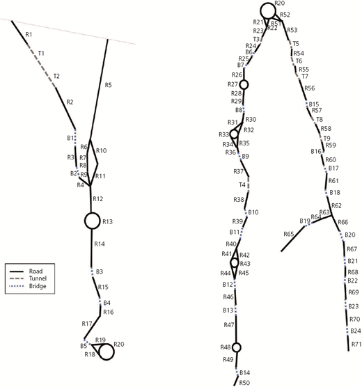
Example network (connected at roundabout R20). Image courtesy of Arnor Elvarsson
Example network (connected at roundabout R20). Image courtesy of Arnor Elvarsson
Road objects in the example network
| Object category | Object | State at year 1 | Length, lo: m | Speed: km/h | Traffic volume: veh/d |
|---|---|---|---|---|---|
| Road sections | R1 | 1 | 218 | 60 | 3000 |
| R2 | 1 | 280 | 80 | 3000 | |
| R3 | 3 | 634 | 80 | 3000 | |
| R4 | 1 | 160 | 80 | 3000 | |
| R5 | 2 | 3300 | 80 | 7000 | |
| R6 | 1 | 215 | 80 | 7000 | |
| R7 | 2 | 25 | 80 | 7000 | |
| R8 | 2 | 164 | 80 | 7000 | |
| R9 | 3 | 43 | 80 | 7000 | |
| R10 | 1 | 397 | 80 | 7000 | |
| R11 | 1 | 43 | 80 | 7000 | |
| R12 | 3 | 179 | 80 | 7500 | |
| R13 | 3 | 69 | 60 | 7500 | |
| R14 | 1 | 595 | 80 | 7500 | |
| R15 | 1 | 2073 | 80 | 7500 | |
| R16 | 1 | 79 | 80 | 7500 | |
| R17 | 1 | 1941 | 50 | 7500 | |
| R18 | 2 | 49 | 80 | 7500 | |
| R19 | 2 | 48 | 80 | 7500 | |
| R20 | 3 | 74 | 80 | 7500 | |
| R21 | 2 | 33 | 80 | 5000 | |
| R22 | 3 | 34 | 80 | 5000 | |
| R23 | 2 | 772 | 80 | 5000 | |
| R24 | 2 | 3005 | 80 | 5000 | |
| R25 | 1 | 760 | 80 | 4000 | |
| R26 | 1 | 430 | 80 | 4000 | |
| R27 | 4 | 55 | 80 | 4000 | |
| R28 | 3 | 86 | 80 | 4000 | |
| R29 | 1 | 654 | 80 | 4000 | |
| R30 | 1 | 387 | 80 | 4000 | |
| R31 | 3 | 39 | 80 | 4000 | |
| R32 | 3 | 38 | 80 | 4000 | |
| R33 | 3 | 75 | 80 | 4000 | |
| R34 | 1 | 24 | 80 | 4000 | |
| R35 | 3 | 22 | 80 | 4000 | |
| R36 | 1 | 3 | 80 | 4000 | |
| R37 | 1 | 80 | 1971 | 4000 | |
| R38 | 1 | 80 | 4557 | 4000 | |
| R39 | 1 | 80 | 1355 | 3000 | |
| R40 | 2 | 80 | 572 | 3000 | |
| R41 | 1 | 80 | 48 | 3000 | |
| R42 | 1 | 80 | 50 | 3000 | |
| R43 | 1 | 80 | 72 | 3000 | |
| R44 | 1 | 80 | 45 | 3000 | |
| R45 | 4 | 80 | 42 | 3000 | |
| R46 | 3 | 80 | 1186 | 2000 | |
| R47 | 3 | 80 | 2559 | 2000 | |
| R48 | 1 | 80 | 69 | 2000 | |
| R49 | 1 | 80 | 191 | 2000 | |
| R50 | 4 | 80 | 37 | 2000 | |
| R51 | 1 | 80 | 33 | 2500 | |
| R52 | 1 | 80 | 31 | 2500 | |
| R53 | 1 | 80 | 3275 | 2500 | |
| R54 | 1 | 80 | 2114 | 2500 | |
| R55 | 1 | 80 | 188 | 2500 | |
| R56 | 1 | 80 | 877 | 2500 | |
| R57 | 2 | 80 | 573 | 2500 | |
| R58 | 3 | 80 | 120 | 2500 | |
| R59 | 4 | 80 | 637 | 2500 | |
| R60 | 1 | 80 | 1628 | 2500 | |
| R61 | 4 | 80 | 2551 | 2500 | |
| R62 | 1 | 80 | 1011 | 2500 | |
| R63 | 4 | 80 | 8 | 2000 | |
| R64 | 1 | 80 | 26 | 2000 | |
| R65 | 1 | 80 | 2955 | 2000 | |
| R66 | 1 | 80 | 3342 | 500 | |
| R67 | 3 | 80 | 1470 | 500 | |
| R68 | 3 | 80 | 251 | 100 | |
| R69 | 1 | 80 | 2125 | 100 | |
| R70 | 1 | 80 | 1972 | 100 | |
| R71 | 2 | 80 | 1610 | 100 |
Bridge and tunnel objects in the example network
| Object category | Object | State at year 1 | Speed: km/h | Length, l o : m | Traffic volume: veh/d |
|---|---|---|---|---|---|
| Bridges | B1 | 2 | 80 | 166 | 3000 |
| B2 | 4 | 80 | 31 | 3000 | |
| B3 | 3 | 80 | 16 | 7500 | |
| B4 | 1 | 80 | 132 | 7500 | |
| B5 | 4 | 80 | 135 | 7500 | |
| B6 | 1 | 80 | 10 | 5000 | |
| B7 | 2 | 80 | 16 | 4000 | |
| B8 | 1 | 80 | 46 | 4000 | |
| B9 | 2 | 80 | 35 | 4000 | |
| B10 | 1 | 80 | 39 | 3000 | |
| B11 | 1 | 80 | 18 | 3000 | |
| B12 | 1 | 80 | 33 | 3000 | |
| B13 | 1 | 80 | 20 | 2000 | |
| B14 | 2 | 80 | 10 | 2000 | |
| B15 | 3 | 80 | 45 | 2500 | |
| B16 | 4 | 80 | 36 | 2500 | |
| B17 | 1 | 80 | 20 | 2500 | |
| B18 | 1 | 80 | 9 | 2500 | |
| B19 | 1 | 80 | 29 | 2000 | |
| B20 | 1 | 80 | 21 | 500 | |
| B21 | 1 | 80 | 40 | 100 | |
| B22 | 1 | 80 | 34 | 100 | |
| B23 | 1 | 80 | 21 | 100 | |
| B24 | 2 | 80 | 32 | 100 | |
| Tunnels | T1 | 1 | 60 | 74 | 3000 |
| T2 | 4 | 80 | 3181 | 3000 | |
| T3 | 1 | 80 | 2248 | 5000 | |
| T4 | 1 | 80 | 59 | 4000 | |
| T5 | 1 | 80 | 131 | 2500 | |
| T6 | 1 | 80 | 219 | 2500 | |
| T7 | 2 | 80 | 79 | 2500 | |
| T8 | 3 | 80 | 49 | 2500 | |
| T9 | 4 | 80 | 378 | 2500 |
Deterioration
The provided service of an infrastructure object is associated directly with the state of the object. In this example, four states are defined – namely, (a) excellent, (b) good, (c) acceptable and (d) poor. The ability to provide service changes over time due to deterioration of the infrastructure – that is, the movement of the object from one state to another. Table 9 shows the probabilities that an infrastructure object changes its state and, therefore, the level of service it provides, from one year to the next. These transition probabilities are reasonable assumptions and differ for different object categories. For example, a road section currently in state 2 has a 75% probability of staying in state 2 and a 25% probability of deterioration to state 3. A bridge, on the other hand, has a probability of 92% of staying in state 2 and a probability of 8% of reaching state 3 in the next year.
Transition probabilities due to deterioration
| Object category | State at year t | State at year t + 1 | |||
|---|---|---|---|---|---|
| 1 | 2 | 3 | 4 | ||
| Road section | 1 | 0·87 | 0·13 | 0·00 | 0·00 |
| 2 | 0·00 | 0·75 | 0·25 | 0·00 | |
| 3 | 0·00 | 0·00 | 0·58 | 0·42 | |
| 4 | 0·00 | 0·00 | 0·00 | 1·00 | |
| Bridge | 1 | 0·96 | 0·04 | 0·00 | 0·00 |
| 2 | 0·00 | 0·92 | 0·08 | 0·00 | |
| 3 | 0·00 | 0·00 | 0·88 | 0·12 | |
| 4 | 0·00 | 0·00 | 0·00 | 1·00 | |
| Tunnel | 1 | 0·99 | 0·01 | 0·00 | 0·00 |
| 2 | 0·00 | 0·95 | 0·05 | 0·00 | |
| 3 | 0·00 | 0·00 | 0·90 | 0·10 | |
| 4 | 0·00 | 0·00 | 0·00 | 1·00 | |
Interventions and intervention strategies
Two intervention strategies (Table 10) are considered for each object type. The strategies denoted A include a minor intervention if an object is in state 3 and a major intervention if the object is in state 4; otherwise, no intervention is executed. Strategies denoted B include a major intervention if the object is state 4; otherwise, there is no intervention. The effectiveness of the interventions, in terms of the probable states following the interventions, and their costs and durations are given in Table 11. The values are based on a report of the Swiss road authority (Herrmann et al., 2008) and expert knowledge.
Intervention strategies with the planned interventions based on states
| Object category | Strategy | State | |||
|---|---|---|---|---|---|
| 1 | 2 | 3 | 4 | ||
| Road section | A | None | None | Minor intervention | Major intervention |
| B | None | None | None | Major intervention | |
| Bridge | A | None | None | Minor intervention | Major intervention |
| B | None | None | None | Major intervention | |
| Tunnel | A | None | None | Minor intervention | Major intervention |
| B | None | None | None | Major intervention | |
Intervention characteristics
| Object category | Intervention type | Possible state of execution | Probabilities of an object to be in state … after an intervention | Intervention cost, : CHF/m | Intervention duration, : h/m | |||
|---|---|---|---|---|---|---|---|---|
| 1 | 2 | 3 | 4 | |||||
| Road | Minor | 3 | 0·7 | 0·3 | 0 | 0 | 338 | 0·026 |
| Major | All | 1·0 | 0·0 | 0 | 0 | 702 | 0·156 | |
| Bridge | Minor | 3 | 0·7 | 0·3 | 0 | 0 | 1820 | 0·5 |
| Major | All | 1·0 | 0·0 | 0 | 0 | 2275 | 1·5 | |
| Tunnel | Minor | 3 | 0·7 | 0·3 | 0 | 0 | 3500 | 1 |
| Major | All | 1·0 | 0·0 | 0 | 0 | 5000 | 2 | |
Impacts on stakeholders and their values
In order to be able to determine the impact of an intervention strategy, the estimation of the impacts has to be defined, including the values associated with them. The cost is estimated for each object individually. The overall cost C o of one specific intervention strategy for one object o is equal to the sum of the cost on object o at each time step t due to all impacts I and the object states s (Equation 1). The cost of impact I of object o in state s consists of two parts.
First, the impact related to the road condition, which is equal to the multiplication of the unit cost ucI of impact I, the unit quantity of object o related to impact I, the factor related to state s of impact I, the duration of 365 d/year and the probability of object o to be in state s in year t.
Second, the impact related to the execution of an intervention, which is equal to the multiplication of the unit cost ucI of impact I, the unit quantity of object o related to impact I, the factor f I-i(s) related to intervention i executed in state s according to the intervention strategy, the intervention duration and the probability of object o to be in state s in year t. Equation 2 shows the combined form.
The factors f I-s and f I-i(s) refer to the change in either unit cost or unit quantity of the impact due to the state s of the road and the intervention executed on objects in state s. They always relate to the difference in cost between the current state and state 1.
Equation 2 is used to estimate the cost related to all impacts. The following subsections identify the equation elements for all stakeholders and all impacts. The unit costs for the different impacts are based on values found in literature. These values refer to the cost in a specific year. All values are converted into 2017 costs by using the customer price index (BFS, 2018).
Owner
As shown in Table 2, the owner impact is equal to the impact of executing interventions in order to maintain an adequate level of service. The cost of executing an intervention could be divided into labour, material and equipment. In this example, they are considered aggregated as intervention cost.
The cost for the owner due to executing intervention i on object o is estimated based on Equation 2. The unit cost for executing an intervention i on an object in state s is expressed in Swiss francs (CHF) per metre of road, bridge or tunnel. Which intervention i is executed on objects of state s depends on the intervention strategy defined. The unit costs for the interventions considered in the example are shown in Table 11. Since the unit cost are defined as monetary units per length, the unit quantity of intervention i on object o is equal to the object’s length lo.
Users
The impacts on the users are accidents, travel time, vehicle operation, comfort and noise emissions (Equation 3). The cost related to each impact is estimated based on Equation 2. The impact for the users due to accidents consists of property damage , injuries and fatalities . Table 12 summarises all impacts and, in particular, shows the associated unit costs.
Impact costs for the users
| Impact I | Unit | Unit cost, ucI: CHF/unit | Unit quantity, : units/d | Factor related to state …, fI-s | Factor related to executing … intervention, fI-i(s) | ||||
|---|---|---|---|---|---|---|---|---|---|
| 1 | 2 | 3 | 4 | Minor | Major | ||||
| Accident | |||||||||
| Damage | Accidents | 42 826 | Equation 4 | 0 | 0·05 | 0·1 | 0·25 | 0·56 | |
| Injury | 41 686 | ||||||||
| Fatality | 51 724 | ||||||||
| Travel time | veh-h | 23·60 | Equation 5 | 0 | 0 | 0 | 0·1 | 0·3 | 1 |
| Vehicle operation | veh-km | 0·58 | Equation 6 | 0 | 0·05 | 0·1 | 0·2 | 0 | |
| Comfort | 0 | ||||||||
| Noise | veh-h | 0·041 | Equation 5 | 0 | 0 | 0·05 | 0·1 | 0 | |
ACCIDENT
The unit cost of the accident impacts is derived from values for property damage, injury and fatality multiplied by the probability of property damage, injury and fatality in case of an accident given by the Swiss norm (VSS, 2013). The unit quantity refers in all three accident impacts to the number of accidents under normal conditions and is equal to the probability of an accident occurring multiplied by the length l o and traffic volume q o on object o (Equation 4). Table 13 provides these values related to accidents. The factors f user.a-s related to the road condition were based on expert opinion, as no such values were found in the literature. It was assumed that the number of accidents increase by 5% on roads in state 2, by 10% on roads in state 3 and by 25% on roads in state 4. In case of an intervention, the accident rate increases by 56% (Bakaba et al., 2012).
Accident probability
| Object type | Probability of an accident per vehicle-kilometre, : × 106 |
|---|---|
| Road | 0·740 |
| Bridge | 0·814 |
| Tunnel | 1·110 |
The probability of an accident occurring depends on the object type. For road sections, the Schweizerischer Verband der Strassen- und Verkehrsfachleute (VSS) norm SN 641 824 provides a value of 0·74 accidents per 1 million vehicle-kilometres (veh-km) travelled (VSS, 2013). Based on a study about road tunnel accidents, it is assumed that the probability of an accident occurring in a tunnel is 50% higher than on an open road, leading to 1·11 accidents per million veh-km (Caliendo and De Guglielmo, 2012). The probability of accidents on bridges is assumed 10% higher than on regular road sections.
Table 14 shows the unit cost estimation for property damage, injury and fatalities for the three stakeholders: users, the directly affected public and the indirectly affected public. The probabilities of property damage, injury and fatality of the users in the case of an accident occurring are based on the norm SN 641 824 (VSS, 2013). The probabilities of property damage, injury and fatality for the directly affected public in the case of an accident occurring are assumed based on the population density. The road is in an area of densities between 3 and 100 people per square kilometre. In such a mountainous area, it is a good assumption that one-quarter of the population lives in close range of the valley road (approximately 10–15 m). This would result in around 1–25 people per kilometre of road. Assuming that an accident on the road does not affect more than 50 m along the road, the probability that the directly affected public is involved in an accident lies around 0·5–12% considering the population density. It is, therefore, assumed that the probabilities of property damage, injury and fatality for the directly affected public due to an accident are 0·12, 0·01 and 0·001, respectively. This is only a simple assumption, which, however, is good enough to show how the directly affected public is affected by road accidents. The indirectly affected public refers to the societal cost of accidents. Therefore, the probabilities for users and directly affected public to be affected by an accident are summed up – that is, the probability of injury affecting the indirectly affected public is the sum of the probability of injury to the users and the directly affected public (0·55 + 0·01 = 0·56).
Unit cost estimation
| Value | Impact | Users | Directly affected public | Indirectly affected public |
|---|---|---|---|---|
| Probability of … in case of an accident | Property damage | 1 | 0·12 | — |
| Injury | 0·55 | 0·01 | 0·56 | |
| Fatality | 0·02 | 0·001 | 0·021 | |
| Cost value | Property damage | 42 826 | 0 | |
| Injury | 75 793 | 16 535 | ||
| Fatality | 2 586 191 | 691 376 | ||
| Unit cost ucI | Property damage | 42 826 | 5139 | 0 |
| Injury | 41 686 | 758 | 9259 | |
| Fatality | 51 724 | 2586 | 14 519 | |
TRAVEL TIME
The unit cost for travel time is 23·60 CHF per vehicle-hour (veh-h) (1 CHF = 1·02 USD) according to the adjusted values given in the Swiss norm (VSS, 2009a). As the unit is related to vehicle-hours travelled, the unit quantity is equal to the travel duration along object o, which is equal to the length l o divided by the speed v o, multiplied by the daily traffic volume q o (Equation 5). The factors f I-s and f I-i(s) have to be assumed, as there is no specific literature about the travel time loss due to the road condition. It is assumed that the travel time increases by 10% due to a poor road condition (state 4) and that the travel time doubles up during a major intervention due to the necessary closure of a full lane on a two-lane road, while minor interventions lead to an increase by 30%.
VEHICLE OPERATING COSTS
The vehicle operation cost adjusted for the year 2017 is expressed in vehicle-kilometres, whereas the unit cost per vehicle-kilometre is 0·58 CHF (Maibach et al., 2006). The unit quantity is equal to the product of the length l o and traffic volume q o on object o (Equation 6). It is assumed that the vehicle operation cost increases by 5, 10 and 20% if the road condition is in state 2, 3 and 4, respectively, due to increased fuel consumption when riding on poor roads.
COMFORT
Regarding comfort, it is assumed that the differences in comfort are low enough to be neglected.
NOISE
The unit cost for noise regarding the users are 0·041 CHF/veh-h travelled (Dykes, 2018; VSS, 2009b). Noise emissions are assumed to increase by 5 and 10% if the road condition is in state 3 and 4.
Directly affected public
The directly affected public is affected by accidents, comfort, noise emissions and particle emissions. The cost for the directly affected public CDAP-o by an object o consists of the summation of the cost of all four impacts (Equation 7). The cost for the directly affected public due to accidents CDAP.a-o consist of the cost of property damage CDAP.pd-o, injuries CDAP.inj-o and fatalities CDAP.fat-o. Table 15 summarises all impacts and, in particular, shows the associated unit costs.
Impact costs for the directly affected public
| Impact | Unit | Unit cost, ucI: CHF/unit | Unit quantity, : units/d | Factor related to state …, fI-s | Factor related to executing … intervention, fI-i(s) | ||||
|---|---|---|---|---|---|---|---|---|---|
| 1 | 2 | 3 | 4 | Minor | Major | ||||
| Accident | |||||||||
| Damage | Accidents | 5139 | Equation 8 | 0 | 0·05 | 0·1 | 0·25 | 0·56 | |
| Injury | 758 | ||||||||
| Fatality | 2586 | ||||||||
| Comfort | 0 | ||||||||
| Noise | veh-km | 2·1 × 10−4 | Equation 9 | 0 | 0 | 0·05 | 0·1 | 0 | |
| Particle emission | veh-km | 0·0104 | Equation 9 | 0 | 0·05 | 0·1 | 0·2 | 0 | |
ACCIDENT
The accident cost related to the directly affected public is estimated similarly to the accident cost for the users shown in the section headed ‘Users’. The difference exists in the probability of property damage, injury and fatality of the directly affected public in case of an accident, which is incorporated into the unit cost values. Further details can be seen in Table 14.
Impacts of noise for the directly affected public differ from the noise impact on the users, as the directly affected public is affected by the surrounding noise of traffic for the entire time, while the users are affected by the in-car noise while driving. The unit cost for the directly affected public due to noise is 2·1 × 10−4 CHF/veh-km (Korzhenevych et al., 2014). The noise increase is assumed to be the same for the directly affected public as for the users with 5 and 10% increases in road states 3 and 4.
COMFORT
The change in comfort for the directly affected public due to a worse road condition is assumed insignificantly small and is therefore set to 0.
NOISE AND PARTICLE EMISSIONS
The unit cost for particle emissions is estimated based on Table 16. The increase in the road condition is assumed equal to the increase in vehicle operation cost, as they are mostly based on the increase in fuel consumption.
Cost of particle emissions
| Emission | Quantity: g/veh-km (Wüthrich et al., 2017) | Cost per tonne: CHF/t (VSS, 2009b) | Cost per vehicle-kilometre: CHF/veh-km | ||
|---|---|---|---|---|---|
| Directly affected public | Indirectly affected public | Directly affected public | Indirectly affected public | ||
| Carbon dioxide | 209 | — | 40 | — | 0·0084 |
| Nitrogen oxides (NOx) | 0·386 | — | 3100 | — | 0·0012 |
| PM | 0·044 | 231 000 | 281 000 | 0·0102 | 0·0124 |
| Total (cost base 2005) | 0·0102 | 0·0219 | |||
| Total (cost base 2017) | 0·0104 | 0·0225 | |||
Indirectly affected public
The indirectly affected public is affected by accidents, socio-economic activities, particle emissions and environment consumption. The cost for the indirectly affected public CIAP-o due to an object o consists of the summation of the cost of all four impacts (Equation 10). The cost for the indirectly affected public due to accidents CIAP.a-o consists of the cost of injuries CIAP.inj-o and fatalities CIAP.fat-o. Table 17 summarises all impacts and, in particular, shows the associated unit costs.
Impact costs for the indirectly affected public
| Impact | Unit | Unit cost, ucI: CHF/unit | Unit quantity, : units/d | Factor related to state …, fI-s | Factor related to executing … intervention, fI-i(s) | ||||
|---|---|---|---|---|---|---|---|---|---|
| 1 | 2 | 3 | 4 | Minor | Major | ||||
| Accident | |||||||||
| Injury | Accidents | 9259 | Equation 11 | 0 | 0 | 0·05 | 0·1 | 0·56 | |
| Fatality | 14 519 | ||||||||
| Socio-economic | 0 | ||||||||
| Particle emission | veh-km | 0·0225 | Equation 12 | 0 | 0·05 | 0·1 | 0·2 | 0 | |
| Environment consumption | 0 | ||||||||
ACCIDENT
The accident cost related to the indirectly affected public is estimated similarly to the accident cost for the users shown in the section headed ‘Users’. The difference exists in the unit costs for injury and fatality, which combine the probability of injuries and fatalities for the users and the directly affected public and multiply them by the societal costs related to injuries and fatalities. Further details can be seen in Table 14.
SOCIO-ECONOMIC ACTIVITY
The change in socio-economic activity due to a worsening road condition is assumed insignificantly small, and, therefore, it was set to 0.
PARTICLE EMISSIONS
The unit cost for particle emissions is estimated using the values given in Table 18.
Transition probabilities due to deterioration
| Object category | State in year t | Strategy A | Strategy B | ||||||
|---|---|---|---|---|---|---|---|---|---|
| State in year t + 1 | State in year t + 1 | ||||||||
| 1 | 2 | 3 | 4 | 1 | 2 | 3 | 4 | ||
| Road section | 1 | 0·87 | 0·13 | 0 | 0 | 0·87 | 0·13 | 0 | 0 |
| 2 | 0 | 0·75 | 0·25 | 0 | 0 | 0·75 | 0·25 | 0 | |
| 3 | 0·70 | 0·30 | 0 | 0 | 0 | 0 | 0·87 | 0·13 | |
| 4 | 1·00 | 0 | 0 | 0 | 1·00 | 0 | 0 | 0 | |
| Bridge | 1 | 0·96 | 0·04 | 0 | 0 | 0·96 | 0·04 | 0 | 0 |
| 2 | 0 | 0·92 | 0·08 | 0 | 0 | 0·92 | 0·08 | 0 | |
| 3 | 0·70 | 0·30 | 0 | 0 | 0 | 0 | 0·90 | 0·10 | |
| 4 | 1·00 | 0 | 0 | 0 | 1·00 | 0 | 0 | 0 | |
| Tunnel | 1 | 0·99 | 0·01 | 0 | 0 | 0·99 | 0·01 | 0 | 0 |
| 2 | 0 | 0·95 | 0·05 | 0 | 0 | 0·95 | 0·05 | 0 | |
| 3 | 0·70 | 0·30 | 0 | 0 | 0 | 0 | 0·92 | 0·08 | |
| 4 | 1·00 | 0 | 0 | 0 | 1·00 | 0 | 0 | 0 | |
ENVIRONMENT CONSUMPTION
The change in environment consumption due to a worsening road condition is assumed insignificantly small, and it was therefore set to 0.
Determination of optimal intervention strategies
The intervention strategy with the lowest cost overall is the one that results in the minimum overall cost
In order to be able to estimate the cost for an object o in time t, the probability of the object to be in a certain state (see Equation 2) is estimated using Markov models. The transition probability p ij refers to the probability of an object of changing from state i to state j within one time step – that is, 1 year. The transition probabilities depend on the deterioration probabilities (Table 9) and the effectiveness of the interventions (Table 11) executed according to the strategy (Table 10) and are considered stationary. The resulting transition probabilities for the two strategies considered in the example are shown in Table 18. The Chapman–Kolmogorov equation (Equation 14) allows the calculation of the transition probabilities of going from state i to state j in t time steps, which is equal to the sum of the probability of going from state i to state k in x time steps multiplied by the probability of going from state k to state j in n-x time steps.
With the Markov model approach, the probability of each object being in each possible state at each year considered can be calculated. Equation 2 then allows the estimation of the cost related to each object for each year. Considering all impacts on every stakeholder, all objects and the entire time period of 30 years, the costs related to the two strategies can be compared. The results are shown in the following section.
Results
It can be seen (Figure 2), assuming that the modelling and input values are correct, that strategy A is better than strategy B. If strategies A and B are followed for all objects, they will lead to cumulative costs of 122 million and 159 million CHF, respectively. The largest cost is due to the interventions executed, as it makes up 63% (strategy A) and 46% (strategy B) of the overall costs. The second largest cost is due to vehicle operation, as it makes up 27% (strategy A) and 39% (strategy B) of the overall costs. The other costs are considerably smaller in magnitude. The fact that the vehicle operation costs are higher than the travel time costs is due to (a) the assumption that the unit cost of travel time is 23·60 CHF/veh-h, which is equal to 0·59–0·20 CHF/veh-km with speeds between 40 and 120 km/h and are therefore smaller than the unit cost for vehicle operation at 0·58 CHF/veh-km, and (b) the assumption that the vehicle operation costs are driven mainly by the state of the object, which affects travel all years, and the travel time costs are driven mainly by the execution of interventions, which are considered only for the duration of the interventions.
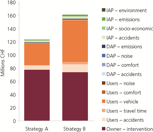
Total costs incurred for strategies A and B. DAP, directly affected public; IAP, indirectly affected public
Total costs incurred for strategies A and B. DAP, directly affected public; IAP, indirectly affected public
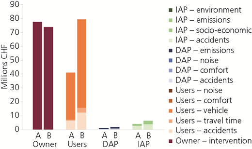
It can also be seen (Figure 3) that the owners and the users incur the most costs of the four stakeholder groups. The minor interventions executed on objects in state 3 in strategy A result in higher costs for the owner than strategy B but users having lower costs due to the road being in poor condition. Although the costs for the directly and indirectly affected public are much smaller than the cost for the owner and the users, they are also higher for strategy B than strategy A.
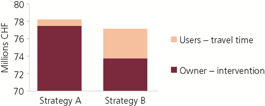
The effect of using this complete service definition can be seen by looking at the intervention strategy that would be selected if only intervention costs and travel time costs were considered (Figure 4). In this case, it can be seen that strategy A results in 77·5 million CHF of intervention costs and 0·7 million CHF of additional travel time costs, whereas strategy B results in 73 million CHF of intervention costs and 3·4 million of additional travel time costs. As strategy B has lower overall costs, it would be selected over strategy A, which is contrary to the choice made if all costs were considered.
Conclusion
In this paper, a definition of road service based on how all relevant stakeholders are affected by the use of the road and the activities to enable the use of the road, in quantifiable units per unit time, is presented (see the section headed ‘Impacts’). This definition of service can be used in consistently and transparently making decisions that affect how infrastructure provides service, such as the determination of optimal intervention strategies for specific assets, optimal intervention programmes for entire networks and the optimal way for interventions to be conducted once it is decided that they should be executed.
It can be seen in the results of the example (see the section headed ‘Example’) that each stakeholder is able to see how the impacts on them were estimated and, given the values placed on each unit, the costs that they are likely to incur if each strategy is followed. Once seeing the results, they might question as to whether they have placed the right values on the impacts per unit time, but they cannot question that their concerns have been adequately taken into consideration. If they do question the values that were placed on the impacts, then the values can be changed and any decisions made with them revaluated. It would be ideal if all road managers had such definitions of service as a basis to enable them to make consistent and transparent decisions in the best interest of all of the stakeholders of road infrastructure.
Although perhaps obvious, something else that is illustrated in the example is that optimal decisions are possible only if the impacts on all stakeholders are considered. The optimal intervention strategy is different if the impacts on all stakeholders are considered or if only intervention costs and travel time costs are considered. Even though the methodology is illustrated on a single example network with relatively homogeneous road characteristics, the methodology can be used to quantify the service on any possible road network – that is, rural roads, highways or mixed networks.
Future work in this area should be focused on the use of this definition in practice where there is interaction with real-world stakeholders of different backgrounds, levels of education and experiences. It is expected that this would involve
considerable discussion of the relationships between the identified costs and the proxies of service often used – for example, reliability
extensive work on the development of ways to obtain the information required to operationalise the definition – for example, how should data be collected to estimate the amount of noise experienced by the directly affected public
investigations into the appropriate ways to be used to place values on the impacts per unit time.
Additional work could be focused on using such a definition of service in the evaluation of road network development strategies, as a step towards uniting the worlds of maintenance and development.
Acknowledgement
The work presented here has received funding from Horizon 2020, the EU’s Framework Programme for Research and Innovation, under grand agreement number 769373.

