When deciding where to build new roads, it would be useful to obtain quickly and reliably an idea of the necessary characteristics of any potential bridges, using limited information and without considerable effort, as there is a considerable amount of information on built bridges in a standardised form, and there are robust algorithms for analysing these data. This study presents a methodology for estimating the likely bridge characteristics using the information available in a bridge database and Bayesian networks. The methodology is demonstrated by estimating the bridge characteristics of 1793 bridge records using nine situational characteristics – for example, the cross-section of the bridge superstructure and number of bridge spans. It is concluded that the methodology is a useful tool when estimating the characteristics of new bridges using only situational information. Compared with naïve-search databases queries, the prediction capability of all networks developed using the proposed methodology showed an estimated accuracy above 86.5%, which is considerably higher than that found when the methodology was not used – that is, 66.5%. Additionally, it is shown that Bayesian networks based on expert experience can obtain results similar to, and in many cases even better than, those of Bayesian networks based solely on learning algorithms.
Notation
- 𝟙
number of counts
- D
data set
- E
evidence
prediction error
cumulative distribution function (CDF) of the empirical CDF
CDF of the ideal CDF
- 𝒢
network structure
maximum a posteriori assignment of x
- K
total iterations of the K-fold validation
- k1
initial number of discretisation intervals of the Hartemink discretisation
- k1
final discretisation intervals of the Hartemink discretisation
- L1
Euclidian norm
- l
pair of adjacent intervals
pairwise mutual information of variable X i for k discretisation intervals
- n
total number of variables
- P
probability distribution
approximation of the probability distribution
- t
fraction of the elements of equal to zero in the critical threshold minimisation problem
fraction t that minimises L 1
- X
given set of random variables X i
- Xi
random variable i
- x
instance of the features of the test data
- x*
configuration of the variables in X that has the highest posterior probability
- y
instance of the response variable of the test data
- Θ
parameters of the network
set of parents of random variables i
Introduction
When deciding where a new road should be built, it is useful to have an idea of the costs of possible routes. To estimate such costs, it is necessary to have some idea about the characteristics of the bridges to be built. One way to do this is to have engineers develop preliminary designs for the bridges that would likely be included in each route. The developed preliminary design, then, stands as a basis for cost estimation and the later, more detailed design of the structure. The establishment of such a preliminary design would, of course, require a significant amount of time and effort. Moreover, such preliminary design cannot be done in the feasibility project initiation phase, when project information is very limited. For this reason, engineers/decision makers tend to use a similar past project as baselines to develop these estimates and evaluate bids or make proposals. However, another way to do this would be to exploit existing historical data of bridges already built in different situations using advanced models, such as Bayesian networks, for prediction. This study examined whether Bayesian networks can be developed to generate reliable and interpretable predictive models effectively for bridge characteristics during the feasibility project phase. The questions that bridge engineers and decision makers would be interested in are, for example, the following:
How many spans should be expected if the bridge is part of a district road and traverses above a train route?
What is the most probable type of a two-span bridge with a 15 m length?
What is the expected depth range of the superstructure given that the maximum length between its piers is 8 m?
What is the most probable combination of the bridge type, its cross-section type and its superstructure depth if it has a 20 m length, a span of 18 m and a 5 m pier height?
It is shown how this can be done using information from an anonymised road information database to estimate bridge characteristics, knowing only the values of a number of characteristics, such as the span to be covered, the functionality of the bridge and the bridge traverses. For that purpose, a methodology for building the optimal Bayesian network that best predicts these variables of interest is developed and examined. The remainder of the paper is structured as follows: The section headed ‘State of the art’ contains an overview of the most common methods used to make predictions in civil engineering and a short review of the state of the art in the prediction of bridge characteristics using these methods. The section headed ‘Methodology of constructing and validating a discrete Bayesian network’ describes the proposed methodology followed in this paper, with a more thorough presentation of Bayesian networks and the required steps to use them to predict bridge characteristics. The section headed ‘Using discrete Bayesian networks and databases’ explains how Bayesian networks and databases can be used to predict bridge characteristics. The section headed ‘Discussion’ contains the main results of this research, as well as a discussion of the limitations of the methodology suggestions for future research. The section headed ‘Conclusion’ contains the conclusions of this study.
State of the art
Methods for making estimates in civil engineering
The access to the structured information has always been an important premise for the civil engineering domain to analyse and synthesise problems and solutions. Specifically, for solving challenging engineering problems, it is necessary to have information related to the past events and initial conditions, such as earthquakes, typhoons, sun intensity profiles, weather profiles and geological conditions. Statistical and probabilistic approaches have been the basis for the development of building safety and reliability codes and standards. The main use cases include, for example, risk and decision analysis, life-cycle analysis, structural reliability and safety factors (Faber et al., 2011).
However, in recent years, there have also been a substantial number of studies focused on exploiting data to make predictions in civil engineering regarding design, material quantities and costs. Researchers make predictions in civil engineering using either stand-alone methods or a combination of them as hybrid models (García de Soto et al., 2017). Some of the most used stand-alone tools for prediction in civil engineering are regression analyses, neural networks, case-based reasoning and Bayesian networks. By using these methods and data, researchers focus on developing decision support systems for predicting values and phenomena, which have high levels of uncertainty and are otherwise very difficult to predict accurately. Some examples of these values and phenomena include project costs at the early project stages, project design at the early stages, delays, safety, project design, road accidents, structural condition and failure of infrastructure systems.
Regression analysis, which has been used to make cost predictions in civil engineering projects since the 1970s, is a statistical method used to reveal relationships between several items. Regression analysis has been used by researchers to predict construction costs in civil engineering projects both directly (Kim et al., 2004; Tam and Fang, 1999) and indirectly by predicting material quantities (Kim et al., 2004). Regression analysis cannot, however, describe effectively non-linear relationships between items and cannot model problems consisting of multiple outputs (Kim et al., 2004).
Researchers have also investigated the application of other methods for making estimates, which can describe non-linear relationships between variables, such as neural networks. Neural networks are mathematical models inspired by the structure of the human brain. Their ability to model non-linear relationships between variables have led the research community to study their use in areas such as the estimation of the cost of infrastructure projects (Hegazy and Ayed, 1998; Kim et al., 2004), infrastructure failure and structural health (Kerwin et al., 2019, 2020). Despite their strong predictive capabilities, artificial neural networks cannot handle noisy data sets, which may cause them to become trapped in local minima (Hegazy et al., 1994). Furthermore, non-experts have difficulty in understanding how they work and often consider them black boxes (Hegazy et al., 1994).
Case-based reasoning, which also originated in the 1970s, is an artificial intelligence (AI) method that makes predictions by reusing and retrieving data from past cases and experiences. For the selection of similar previous cases, statistical measures are used. Building cost estimation (García de Soto and Adey, 2015; Kim et al., 2004) and early-stage building design (García de Soto et al., 2020) are example areas where case-based reasoning has been used. The main weakness of using case-based reasoning is that the success of a prediction is based on the suitability of the solutions found in the retrieved cases (García de Soto et al., 2020). Additionally, there is a possibility that similar past cases may not exist, which means that there will be either poor predictions or no predictions at all.
Bayesian networks are directed acyclic graphs of uncertain quantities that describe probabilistic relationships between variables within a set of variables. Bayesian networks are a powerful tool for decision making under uncertainty. They have been used in research in a wide range of engineering applications, such as the prediction of road accidents (Deublein et al., 2013), the estimation of bridge condition (Rafiq et al., 2015), the estimation of engineering risk (Delgado-Hernández et al., 2014), the estimation of schedule risk (Luu et al., 2009) and the estimation of project budget risk (Khodakarami and Abdi, 2014). Some of the advantages of Bayesian networks (Luu et al., 2009) include the fact that there are no specific input and output variables. In contrast to other methods such as neural networks and regression analysis, the model is updated, and inference is performed when a new value of a variable is available. Additionally, the model can be updated when new information is available and does not need reconstruction, and due to the graphical display, the relationships between variables can be understood by non-experts. Table 1 gives an overview of the tools mentioned earlier and the weaknesses in using these tools to make estimates pertaining to civil engineering structures.
Examples of the most common prediction tools in civil engineering
| Tool | Prediction | Reference | Weakness |
|---|---|---|---|
| Regression analysis | Concrete cost estimation | Tam and Fang (1999) | Inappropriate when describing non-linear relationships, consisting of multiple inputs and multiple outputs (Tam and Fang, 1999) |
| Material quantity estimation | García de Soto et al. (2014) | ||
| Building cost estimation | Kim et al. (2004) | ||
| Neural networks | Road accidents | García de Soto et al. (2018) | Lose their effectiveness when the patterns are very complicated or noisy, the problem representation and problem structuring are ill defined and training may be trapped in local minima; long computational time (Hegazy et al., 1994); model needs to be retrained when new information is available (Hong et al., 2002) |
| Cost estimation of projects | Hegazy and Ayed (1998), Kim et al. (2004) | ||
| Pipe failure prediction | Kerwin et al. (2019) | ||
| Structural health monitoring | Neves et al. (2017) | ||
| Case-based reasoning | Building cost estimation | García de Soto and Adey (2015, 2016), Kim et al. (2004) | Limitations to reflect suitable search criteria to index and match depending on previous experience without validating them in a new situation |
| Building design | García de Soto et al. (2020) | ||
| Bayesian networks | Occurrence of road accidents | Deublein et al. (2015, 2013) | Difficulty in developing a Bayesian network with both discrete and continuous variables (Deublein et al., 2013). Current Bayesian network applications handle mostly discrete variables (Hu and Mahadevan, 2018). A vast amount of data may be needed for the learning of the network (Delgado-Hernández et al., 2014) |
| Project cost risk analysis | Khodakarami and Abdi (2014) | ||
| Bridge condition modelling | Rafiq et al. (2015) | ||
| Risk assessment | Delgado-Hernández et al. (2014) | ||
| Quantifying schedule risk | Luu et al. (2009) |
Preliminary bridge design estimates
Although some researchers have been exploiting data and have used statistical, machine learning and AI techniques to make predictions in civil engineering, little research has been conducted regarding preliminary bridge design and prediction of bridge characteristics using these tools in recent years. Reich (1996) presented several advancements for the conceptual and preliminary design of bridges, using mostly expert systems, but since then, limited research has been conducted in this area. This probably happened because the developed expert systems did not reach their full potential (Boussabaine, 1996). In some cases, such as project cost estimation, this has led to case-based reasoning systems being used instead (Kim et al., 2004).
Table 2 provides an overview of previous investigations after 2000 related to predicting bridge design and/or specific bridge characteristics using the methods presented in Table 1. Specifically, Hong et al. (2002) applied multilevel neural networks for performing preliminary bridge design. Their research concluded that neural networks are suitable for modelling past experience for prediction of bridge elements in the preliminary design stage. Andrade et al. (2003) developed a model, framework and system that integrated case-based reasoning and neural networks for design and tested it successfully on highway bridge projects. They obtained the dimensions of bridge elements that were similar to actual values. However, Singer et al. (2016) outlined in their research that the process of a holistic preliminary bridge design is too complex to be represented with what-if rules. They attributed this to the fact that bridge design consists of several design elements, including the superstructure, substructure, foundation, abutments, bearings, bridge equipment, materials and construction methods, which are dependent on boundary conditions, such as the required bridge alignment, the traffic type to be carried and the existing terrain and soil conditions. They also pointed out that Bayesian networks may be the most suitable tool to be used to predict bridge characteristics based only on situational information. Jootoo and Lattanzi (2017) compared the use of Bayesian networks, decision trees and support vector machines for the prediction of bridge type using bridge characteristics, including the material type, average span length, deck structure and maximum span length. They obtained results that were similar to the actual bridge type and concluded, among other things, that Bayesian networks were a useful tool to predict both bridge type and conceptual bridge design.
Previous studies on preliminary bridge design and prediction of bridge characteristics using the tools in Table 1
| Author | Prediction | Tools | Result |
|---|---|---|---|
| Hong et al. (2002) | Preliminary structural design of cable-stayed bridges | Neural networks | Multilevel neural networks for preliminary structural design; initial input: bridge length, clear height, bridge width |
| Andrade et al. (2003) | Design of highway bridges | Case-based reasoning (CBR), neural networks | A model, a framework and an implemented system for design integrating CBR and machine learning tools such as neural networks; results similar to real values |
| Jootoo and Lattanzi (2017) | Bridge type classification | Bayesian networks | Artificial approaches can be used to predict bridge type in the preliminary design phases; four input variables: material type, average span length, deck structure type, maximum span length |
| Singer et al. (2016) | Bridge characteristics | Bayesian networks | Bayesian networks seem suitable for preliminary bridge design; no real data were utilised |
The suitability of Bayesian networks in representing well-posed problems, where the distribution of each parameter is known and their uncertainty can be quantified (Khodakarami and Abdi, 2014), as well as their potential to model causal relationships between the design parameters and situational characteristics (Matthews, 2008), makes their further use in bridge design worth exploring. As can be seen from Tables 1 and 2, although many people have used Bayesian networks in many civil engineering situations, no one has yet explored the possibility of developing and testing a methodology for predicting future bridge characteristics based only on situational ones, merely by exploiting information from existing bridge databases. With this in mind, the work presented in this paper is intended to fill this gap – that is, compare several learned network structures and logically constructed networks from expert experience and ultimately form a robust Bayesian network that makes accurate estimations in the early stages of a project for some bridge components (e.g. cross-section depth) using only the values of a number of other characteristics, such as the span to be covered, the functionality of the bridge or what the bridge traverses.
Methodology of constructing and validating a discrete Bayesian network
Bayesian networks are probabilistic graphical models that represent a set of random variables and their conditional dependencies by way of directed acyclic graphs. The arrows between two variables show the direct influence of a node A on node B, where a node represents a discrete or continuous random variable. A Bayesian network estimates the joint probability distribution (global distribution) of the random variables using the products of the conditional probability distributions of each variable (local distributions). In the case of discrete variables, the joint probability distribution P of n variables in total is given by the equation
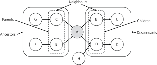
where (or Πi for the sake of clarity) is the set of the parents of Xi. The ancestors, parents, descendants and children of a node A in a Bayesian network are shown in Figure 1.
For a detailed description of the theory and the implementation of Bayesian networks, the reader is referred to the books by Koller and Friedman (2009), Nielsen and Jensen (2009) and Nagarajan et al. (2013).
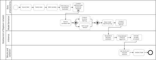
Figure 2 shows the methodology described in this section and followed in this research. The methodology consists of four main stages: data processing, model formation, inference and results/model validation.
Data preprocessing
As this methodology is entirely based on data, a sufficient and reliable data set with information about relevant problem variables needs to be acquired.
The model variables need to be determined. For the determination of the model variables, those that are the most likely to contribute the most to predictions are chosen.
The third step consists of the removal of incomplete observations – that is, observations that contain non-assigned values (‘N/A’) to provide a complete data set and without duplicate observations – that is, observations that are registered more than once to avoid undesired biases in the interdependencies of the data.
To overcome the obstacles imposed by the presence of continuous variables in the network and the fact that a variable distribution departs significantly from normality (e.g. skewness), one solution is to use discretisation and convert these variables into binomial or multinomial distributions. Researchers (Fayyad and Irani, 1993; Friedman and Goldszmidt, 2000) have discussed several methods in order to choose the interval of each state: marginal discretisation methods such as equidistant intervals or equiprobable intervals or other discretisation methods such as Hartemink’s discretisation (Hartemink, 2001) that balances accuracy and information preservation. Furthermore, merging of states (levels) of variables should be applied in case of a large number of states to reduce problems related to network modelling. The large number of states increases the total number of parameters of the network and, therefore, affects the complexity of the network and the correct estimation of the values of its parameters.
Model formation
In Bayesian networks, the directed graphical structure of the network model can be determined either by expert knowledge or by learning algorithms, which build (learn) the network model structure from the data. In any case, the final model should be compared with other candidate solutions.
Structure based on expert experience
Directed arcs in Bayesian networks simply denote the conditional independence relationship between variables, without any strict implications that the arcs should represent cause–effect relationships. However, it can be argued (Pearl, 2009) that a ‘good’ Bayesian network has to indicate the causal structure of the data it is describing. Such Bayesian networks are usually fairly sparse, and their interpretation is, at the same time, clear and meaningful. This is the reason why the formulation of a Bayesian network from expert knowledge is preferred, as it codifies in practice known and expected causal relationships for a given phenomenon. In general, it is not possible to identify a single ‘best’ causal Bayesian network but rather deduct a small set of likely causal Bayesian networks that best fit knowledge of the data.
Structure based on learning algorithms
To examine how well the proposed network complies with reality, it should be compared with other network structures, which can automatically be derived from the data. For learning the structure of a Bayesian discrete network, several algorithms can be deployed. These algorithms can be grouped into three broad categories: (a) constraint-based algorithms, (b) score-based algorithms and (c) hybrid algorithms. More information about these algorithms can be found in the paper by Puga et al. (2015).
Parameter learning
Since the network structure and its number of parameters are known, the values of these parameters can be estimated. There are two main approaches to estimate these parameters: (a) maximum likelihood estimation and (b) Bayesian estimation (Nagarajan et al., 2013). However, maximum likelihood estimation poses limitations. If the database is sparse or a multivariate problem is considered, the maximum likelihood estimate will be equal to zero and will result in a transition probability equal to zero, which may contradict knowledge in the field (Nielsen and Jensen, 2009). Thus, to overcome this limitation, Bayesian parameter estimation is used.
Model inference
Phase 3 concerns the Bayesian inference of the model. Bayesian inference deducts the state of a variable or a set of variables given as evidence of the state of others. The inference uses the network structure and the conditional probability tables for propagating the observed information of the evidence through the network to calculate the probability distribution of the response variables. Conditional to the network complexity, exact or approximate inference can be employed. While exact inference algorithms – like belief propagation or junction trees – combine repeated applications of Bayes’ theorem with local computations to obtain the exact value of the evidence-dependent variable state, for approximate inference, sequential Monte Carlo simulations to sample from the global distribution and thus estimate the posterior distribution can be deployed. The random samples, which are subjected to some conditions and are generated from this process, are also known as particles, and the algorithms that make use of them are known as particle filters. The most notable from them are logic sampling (Henrion, 1988) and likelihood weighting (Dagum and Luby, 1993).
As far as queries are concerned, this research focuses on maximum a posteriori (MAP) queries, also known as most probable explanation queries. These queries, which are provided in Equation 2, are concerned with finding the configuration of events that yields the highest posterior probability.
where x is a specific combination of one or more variables in X, E are the evidence variables, is the network model and Θ are the parameters of the model.
Model validation
One effective method to validate different machine learning models is cross-validation. By using cross-validation, the data set is divided into two subsets: train and test sets. The most powerful cross-validation method is K-fold cross-validation (Herlau et al., 2016). In K-fold cross-validation, the data set is split into K subsets of equal size. In the next step, the model is trained on K − 1 subsets and then tested on the remaining subset. The same procedure is repeated K times. Researchers have suggested that a number of folds K = 10 can provide accurate results (Kohavi, 1995).
For the quantification of a discrete Bayesian network model performance, the prediction error will be used as a metric. The prediction error , which is described in Equation 3, shows how well each network structure can predict the value of a variable of interest, given a particular instance of a subset of the remaining variables and a training set.
which is the probability, of all (x, y) pairs sampled from P, that the classifier selects the wrong label.
Using discrete Bayesian networks and databases
Data preprocessing
Data acquisition
The data were collected from a road-bridge database, which serves as the unique source for the network formation. In the back end, the database consists of a list of entries. Each of them represents a single bridge, for which several attributes are assigned. The data can be presumed as a two-dimensional matrix, in which each row i represents a single observation – namely, the bridge instance – and each column j corresponds to the bridge attribute (variable of interest) used to examine the bridge. The cell ci,j denotes the particular assignment of variable j for the ith bridge. The data set consists of 1793 instances with 17 different variables of interest, both categorical and numerical.
Determination of variables and state merging
To test the methodology, it was decided to create a simple model, containing only the variables of higher importance. Not all variables were considered helpful in modelling. The reasons for their removal were the following.
They play at most a minor role in the bridge design process. The variables with no role or only a minor role are bridge identity, bridge crossing angle, slope, transverse inclination, curvature and the maximum superstructure cross-section depth, as their difference with the respective minimum depth is – if not negligible – smaller than 40 cm in 90% of the cases. Their inclusion in the model would impose difficulties in the accurate estimation of the model parameters, given the limitations of the available data.
They do not have a sufficient number of entries. There were insufficient data for the construction process of the superstructure, for which only half of the bridges have values.
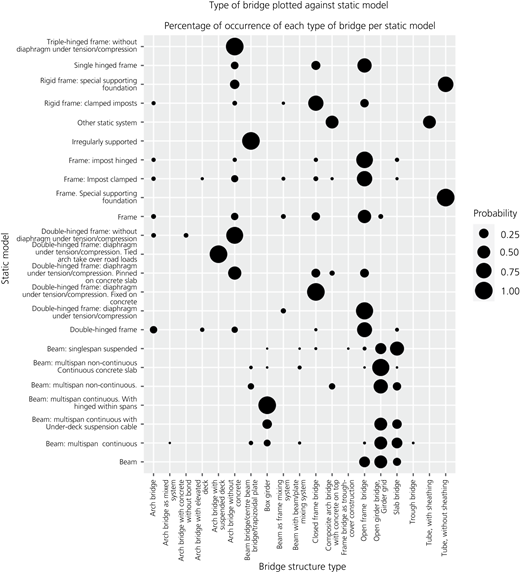
They are strongly – nearly one to one – correlated with other variables. For example, the variable static system was strongly correlated with bridge type. Bridges that are statically modelled as double-hinged arc frame and bar under tension or compression or arc frame clamped in its foundations or simple arc frame or single-hinged arc frame are all categorised as frame bridges in terms of their bridge type (see the Appendix (which also includes Figure 12) for more information).
Additionally, some categorical variables were removed to increase the statistical relevance of each remaining categorical variable. An example of such an occurrence shall be observed in a part of the initial levels of the superstructure cross-section type: the levels ‘single-celled hollow box’, ‘single-celled hollow box, walkable’, ‘single-celled hollow box, crawlable’, ‘single-celled hollow box, non-walkable, non-crawlable’ and ‘superstructure as a hollow box’ can all be assigned to the same level named ‘hollow’, as they are semantically equivalent to each other.
Discretisation of numerical variables
The steps used to determine the variable to be used in the model development variables were as follows:
Removing all entries with not assigned values. This resulted in almost 16% of all instances being removed (approximately 1500 instances).
Using Hartemink’s discretisation algorithm. Hartemink’s discretisation algorithm takes as input a data set of continuous variables = Xi, I = 1, … N, and yields a data set with N discrete variables, each with k2 levels, preserving as much mutual information between variables as possible. The algorithm is executed as in Table 3.
Hartemink’s discretisation algorithms
| Input | A data set D of continuous variables, k1 – that is, the initial (large) number of discretisation intervals – and k2, the final discretisation intervals |
| Output | A discrete data set of factor variables, each discretised in k2 levels in total |
| Initialisation | |
| Discretise each variable independently using quantile discretisation and a large number k1 of initial intervals | |
| Specify the desired number of states of the variables in the end k2 | |
| Fork = k1; k2 + 1; k = k − 1 do | |
| Fori ← 1 to Ndo | |
| Compute pairwise mutual information coefficients: | |
| Foreach pair l of adjascent intervals of Xido | |
| Collapse each pairlof adjacent intervals of Xi in a single interval, and from the resulting variable compute: | |
| End | |
| Set | |
| End | |
| End | |
After this step, nine of the original 17 variables remained for the development of the Bayesian network model (Table 4). The discrete states for each selected variables are also shown in Table 4.
Bridge attributes, their respective names for the modelling and their discrete states
| Bridge attribute | Variable name | Discrete states |
|---|---|---|
| Which operation does the bridge fulfil? | Operation | Autobahn (highway without a speed limit) |
| Federal highway | ||
| Other street | ||
| Cycling path | ||
| District road | ||
| State road | ||
| What is lying underneath the bridge? | Underneath | Highway |
| Typical street | ||
| River | ||
| Small intervention | ||
| Train | ||
| How long is the bridge in metres? | Bridge_length | [1.6; 4.28] |
| (4.28; 8.26] | ||
| (8.26; 14.5] | ||
| (14.5; 45.5] | ||
| (45.5; 1.02 × 10³] | ||
| How high is the highest bridge pier in metres? | Pier_height | [0; 1] |
| (1; 3] | ||
| (3; 4.6] | ||
| (4.6; 6.5] | ||
| (6.5; 78.6] | ||
| How many are the spans of the bridge? | Span_No | 1 span |
| 2 spans | ||
| >2 spans | ||
| Which is the structure type of the bridge? | Bridge_type | Beam bridge |
| Arch bridge | ||
| Frame bridge | ||
| Plate girder | ||
| How long is the maximum span length in metres between consecutive piers of one bridge? | Max_span_length | [0.7; 3.4] |
| [0.7; 3.4] | ||
| (7.78; 13] | ||
| (13; 22.9] | ||
| (22.9; 171] | ||
| Which is the cross-section type of the superstructure? | Cross_section_type | Single girder |
| Hollow | ||
| Other | ||
| Multiple girders | ||
| Which is the minimum depth in metres of the superstructure cross-section (typically in the bridge middle)? | Cross_section_depth | (0.1; 0.49] |
| (0.49; 0.6] | ||
| (0.6; 0.9] | ||
| (0.9; 1.42] | ||
| (1.42; 7.25] |
Model formation
The model formulation consists of two parts, (a) the model structure and (b) the parameters. To determine the optimal model structure, expert opinion, based on the bridge design process, was first used (see the section headed ‘Model structure based on expert experience’) and then compared with the results of the model structure determined using seven structure-learning algorithms (see the section headed ‘Model structure based on learning algorithms’).
Model structure based on expert experience
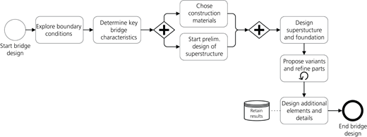
The structure of the Bayesian network was determined based on expertise, using the proposed concept for preliminary bridge design developed by Singer (2014) (Figure 3) and the variables and correlations identified in the section headed ‘Data preprocessing’.
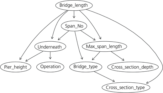
The exact interactions between the model variables are shown in the proposed model in Figure 4, where the arcs denote the direct causal influences between the nodes. The nodes represent variables used in the bridge design process that are
external to the bridge design process – that is, ‘Operation’ and ‘Underneath’
dependent solely on the situational variables – that is, ‘Bridge_length’ and ‘Max_span_length’
dependent on both internal and external variables – that is, ‘Span_No’ and ‘Pier_height’
dependent on internal variables – that is, ‘Bridge_type’ ‘Underneath’, ‘Operation’, ‘Span_No’, ‘Cross_section_type’ and ‘Cross_section_depth’.
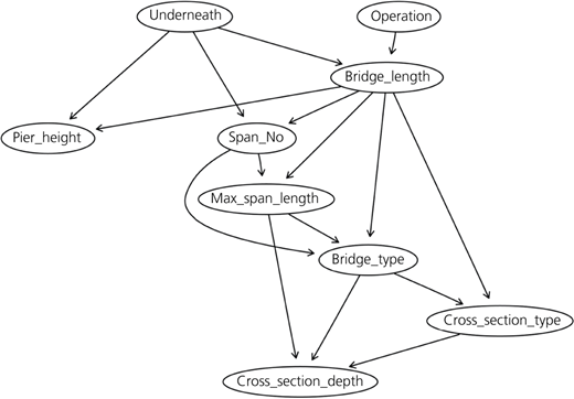
It is noted that other models are possible, meaning that the engineer or the project manager subjectively chooses the design steps of the structure based on engineering intuition. However, since the design of a structure, including bridge structures, is not a linear but an iterative process with many variables, similar models can be suggested. This constructed model, however, referred to herein as the ‘proposed model’, is based on key bridge design steps, derived from Singer’s research, and exploits the most significant conditional dependencies between the available variables. It could be argued that some variables such as bridge crossing angle and curvature could be in certain situations important; they introduce torsion, which affects the cross-section type and cross-bracing.
Model structure based on learning algorithms
To learn the structure of the network only based on the available data, seven structure-learning algorithms from the three categories were used:
constraint-based algorithms such as grow–shrink (Margaritis, 2003), incremental association (IAMB) (Tsamardinos et al., 2003), fast incremental association (fast-IAMB) (Margaritis, 2003) and interleaved incremental association (inter-IAMB) (Yaramakala and Margaritis, 2005)
score-based algorithms such as hill-climbing and Tabu search (Bouckaert, 1995)
hybrid algorithms such as max–min hill-climbing (MMHC) (Tsamardinos et al., 2006).
For computing the different network structures based on the aforementioned learning algorithms, the ‘bnlearn’ R package was used (Scutari, 2010).
Figure 5 shows the networks learned from the road database through constraint-based algorithms. Despite the validity and the robustness of these algorithms, the obtained results are far from satisfactory and are in complete contrast to the interdependencies based on the proposed network in Figure 4. All these learned structures show that there are variables that are independent of all the others in the network and therefore should be eliminated. This can be observed in Figure 5, as there are nodes in all cases that are not connected with the others.
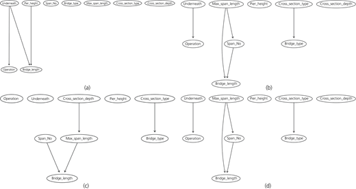
Learned networks through the constraint-based learning algorithms: (a) grow–shrink; (b) incremental association Markov blanket; (c) fast incremental association Markov blanket; (d) interleaved incremental association Markov blanket
Learned networks through the constraint-based learning algorithms: (a) grow–shrink; (b) incremental association Markov blanket; (c) fast incremental association Markov blanket; (d) interleaved incremental association Markov blanket
Figure 6 shows the learned network graphs based on the score-based algorithms: hill-climbing and Tabu search (Bouckaert, 1995). The obtained network graphs match better the graph structure of the proposed network, including interdependencies that are mostly reasonable. For instance, bridge length plays an important role in the estimation of almost all other variables in both these network structures. However, differences can still be observed. For instance, the variables ‘Operation’ and ‘Underneath’ are considered here to be dependent on one another in both graphs, a relationship that in the real world is non-sensical.
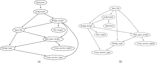
Learned networks through the score-based learning algorithms: (a) hill-climbing algorithm; (b) Tabu-search algorithm
Learned networks through the score-based learning algorithms: (a) hill-climbing algorithm; (b) Tabu-search algorithm
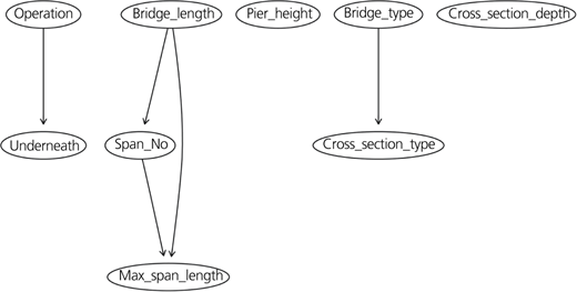
Figure 7 shows the learned network graph based on the applied hybrid algorithm max–min climbing. It can be seen that the variables ‘Pier_height’, ‘Operation’ and ‘Underneath’ are considered independent from all the other variables and are excluded from the learned network graph.
It is noted, though, that all the above-generated networks depend significantly on their initialisations and may be prone to ‘noise’ resulting from the unsystematic correlation within the data. It can be the case that the main relationships are going to be missed that way. To de-noise the learned networks and form a more stable one, it is also worth creating a model averaging network produced from multiple networks, as researchers have proved that it can result in a better predictive performance than choosing a single, high-scoring network (Claeskens and Hjort, 2008). The higher predictive accuracy of the averaged network can be explained from the consensus implemented between all the possible single networks.
The structure of this network is learned by repeating several times the hill-climbing structure-learning algorithm (bootstrapping resampling technique) with different initialisations. In this way, a larger number of network structures could be explored in an effort to reduce the impact of locally optimal (but globally suboptimal) networks on learning and subsequent inference. The averaged network structure was created using the arcs present in at least a specified ratio of the networks. The so-called strength of each arc measured by this proportion provides the means to establish its significance given a threshold.
The critical threshold was computed as a minimisation problem of the Euclidian norm (L1 norm) (Nagarajan et al., 2013):
where is the cumulative distribution function (CDF) of the computed arc strengths (empirical CDF) and is the CDF of the ideal network (ideal CDF), in which the t fraction of the elements of equals 0 and the rest equals 1. It is a measure of the fraction of non-significant edges. At the same time, t provides a threshold for separating the elements of . The identification of significant edges can be thought of as either a least absolute deviation estimation or an L1 approximation:
For the bridge network, the significance threshold equals 0.444, meaning that the averaged graph was created using the arcs present in at least 44.4% of all the networks generated.
Parameter learning
Bayesian estimation was used for parameter learning by assuming a uniform prior of the probabilities. Hyperparameter a of the prior was chosen equal to 1. An example of the conditional probabilities of the proposed network for the cross-section type variable is shown in Figure 9.
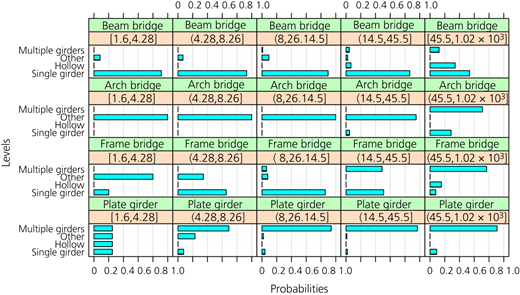
Conditional probability of the ‘Cross_section_type’ variable calculated through Bayesian estimation for the expert network. According to this, the parents of the ‘Cross_section_type’ are ‘Bridge_type’ and ‘Bridge_length’
Conditional probability of the ‘Cross_section_type’ variable calculated through Bayesian estimation for the expert network. According to this, the parents of the ‘Cross_section_type’ are ‘Bridge_type’ and ‘Bridge_length’
As described in the section headed ‘Model formation’, one additional imaginary observation is assumed for each state of the variables. The reason this is done is twofold: firstly, to avoid overfitting of the model on the data set, and secondly, for the estimation of parameters with no data, equal, non-zero parameters are assigned to each state. This is clearly highlighted in Figure 9: there are no instances in the data indicating a plate girder bridge with a length between 1.6 and 4.28 m. Instead of assigning null posterior probabilities to the states of the cross-section type, it is assumed to be a uniform prior distribution.
Model inference
From the available methods described in the section headed ‘Model inference’, logic sampling and likelihood-weighting approximate inference algorithms were used to infer the proposed network structure. The algorithms were examined regarding their accuracy with an increasing number of particles. Figures 10(a) and 10(b) show the estimated probability of the bridge type being a ‘plate girder’, given that the number of spans is greater than two, using increasing sample sizes (particles), where 20 simulations were run for each of sample size (ranging from 5000 to 100 000 particles in increments of 5000). Both inference methods converged to the same accurate result with increasing sample sizes – that is, a high number of particles. The likelihood-weighting algorithm, however, converged more rapidly to the solution, as it is close to the true value already from 5000 particles. The logic sampling algorithm exhibited a relatively large discrepancy of the iterations per number of particles, and their mean value initially deviated from the true value of the conditioned event. The likelihood-weighting algorithm was, therefore, used for all the subsequent calculations.
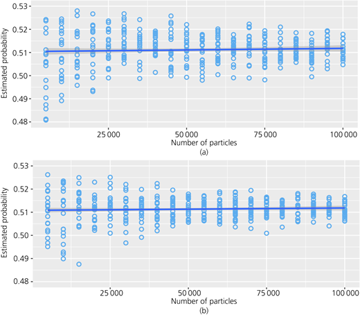
Probability of bridge type = ‘plate girder’ conditioned on evidence Span_No = ‘>2 spans’ (a) using logic sampling and (b) using likelihood weighting
Probability of bridge type = ‘plate girder’ conditioned on evidence Span_No = ‘>2 spans’ (a) using logic sampling and (b) using likelihood weighting
An example using the variables bridge type (‘Bridge_type’), cross-section type (‘Cross_section_type’) and superstructure depth (‘Cross_section_depth’), which are most often subjected to change during designing and dimensioning of the bridge, is given in Table 5. It shows the five most likely combinations for the specific set of evidence and their probability of occurrence. From Table 5, it can be seen that if the maximum span between the piers is between 18.2 and 22.9 m, the bridge length is between 14.5 and 45.5 m, the number of spans is 1 and the maximum pier height is between 4.6 and 6.5 m, the most likely bridge is a plate girder bridge with a multiple girder cross-section and a superstructure depth between 0.9 and 1.42 m with a probability of 54.98%. If the information in the network was sparse, then there would be observed a small correlation between the variables. This would yield to almost random transitions from one variable to another, resulting in several possible design combinations all having the same probability; this was not the case in the proposed network, as the assumptions of correlation and causation were satisfied. Thus, the obtained results from this MAP query were meaningful.
Best sampling results of the expert (proposed) network for maximum span length = (18.2; 22.9) (m), bridge length = (14.5; 45.5] (m), number of spans = 1 and maximum pier height = (4.6; 6.5] (m)
| ID | Bridge type | Cross-section type | Cross-section depth: m | Probability: % |
|---|---|---|---|---|
| 1 | Plate girder | Multiple girders | (0.9,1.42] | 54.98 |
| 2 | Beam bridge | Single girder | (0.9,1.42] | 9.98 |
| 3 | Plate girder | Multiple girders | (0.1,0.49] | 8.09 |
| 4 | Beam bridge | Single girder | (0.6,0.9] | 5.56 |
| 5 | Frame bridge | Single girder | (0.6,0.9] | 2.68 |
Model validation
To validate the proposed model, K-fold cross-validation was used as described in the section headed ‘Model validation’. A tenfold cross-validation was performed; after having split the data into ten equally sized random sets, the model was trained in each iteration on a subset of 90% of the instances and tested on the remaining 10% (≈150 instances). Ten such iterations were performed, and the prediction results were averaged. The results are shown in Figure 11, where the log-loss – that is, the negated expected log-likelihood – of the network is presented. The loss of the whole network is defined as the sum of the log-loss of each variable independently. The log-loss function is applied to the test set for the Bayesian network fitted from the training set. The objective is to minimise the log-likelihood, and this is best achieved for the averaged network. The two score-based algorithms follow with an almost identical loss between each other and slightly higher than that from the averaged network. The proposed network follows with a 4% higher loss relative to the averaged network. All the constraint-based and hybrid algorithms follow with significantly lower predictive capability. Their loss increase ranges from 23 to 42% when compared with the averaged network loss. It can be argued that the reason for their ill performance is the low degree of connectivity between variables, as Figures 5 and 7 indicate.
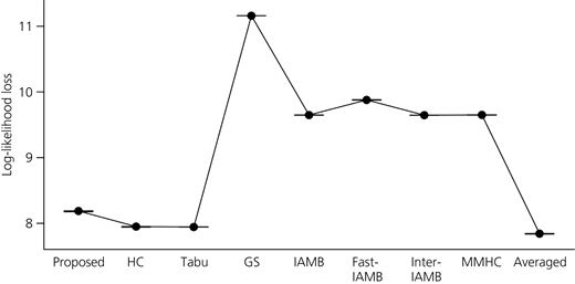
Tenfold cross-validation of learning algorithms. The figure shows the log-loss values for each network. HC, hill-climbing; GS, grow-shrink
Tenfold cross-validation of learning algorithms. The figure shows the log-loss values for each network. HC, hill-climbing; GS, grow-shrink
However, the inference of some variables is more interesting than those of others; therefore, one may want to examine the predictive performance for these variables of interest specifically. For example, it only makes sense to estimate the cross-section depth of a bridge based on situational characteristics such as the object underneath, the height of the piers or the purpose that the bridge fulfils, rather than the opposite. Table 6 shows the mean posterior classification error for predicting the variables ‘Bridge_type’, ‘Cross_section_type’ and ‘Cross_section_depth’ among the proposed network and the best learned networks (Tabu search, hill-climbing, model averaging) by deploying tenfold cross-validation. The results in Table 6 show that the proposed network has the lowest classification error among the network structures shown for predicting all three variables. This comparison strengthens the authors’ assumption that the proposed network is not only more sensible in its construction but also demonstrates superior behaviour compared with the other learned networks.
Posterior classification error in percentage for the variables ‘Bridge_type’, ‘Cross_section_type’ and ‘Cross_section_depth’ among the generated networks
| Network | Bridge type | Cross-section type | Cross-section depth |
|---|---|---|---|
| Proposed | 22.7 | 14.0 | 36.1 |
| Hill-climbing | 24.1 | 15.5 | 40.2 |
| Tabu search | 24.3 | 15.5 | 40.2 |
| Averaged | 24.4 | 15.8 | 40.2 |
Furthermore, the prediction error from the different networks was also compared with a naïve predictive model, which used only the database as a predicting tool. The naïve predictive model had no graphical representation of the variables and merely classified the variable of interest using only the database by the elimination of all non-matching cases, according to the equation
For instance, the ‘Cross_section_type’ variable was predicted according to the level that yielded the highest probability in the database for a specific combination of the levels of all the possible evidence. To compare this naïve model with the aforementioned ones, tenfold cross-validation was conducted to calculate the prediction error only for the ‘Cross_section_type’ variable. The naïve model resulted in a prediction error for the same variable equal to 35.9%. This means that if one would try predicting the type of the cross-section only by using the data set and eliminating the instances for which the evidence does not match exactly, then one would have 35.9% wrong classifications on average. This error rate is significantly higher than the result yielded from most of the graph structures. Specifically, the predictive capability of this model is 64.1% accurate for the variable ‘Cross_section_type’, whereas all the other Bayesian network models showed an increased accuracy up to 86.0% for the same variable of interest.
Discussion
Contribution to research and practice
The use of Bayesian networks as a support tool to determine the bridge characteristics during the early phases of a project has proven to be feasible and can provide useful results with little effort by exploiting existing data. Nevertheless, the best way to interpret the above results is by observing not only the best candidate options but also how the set of the boundary conditions (evidence) excludes some antagonistic solutions. The Bayesian inference indicates the most possible set of solutions – for instance, bridge type or depth of the superstructure cross-section for a specific set of evidence – acting as a decision support tool. Engineers should, however, not take these sets of solutions for granted but should focus their attention on why the inference showed these results and excluded others.
Another advantage of using of the proposed approach is that it drastically increases the engineers’/designers’ ability to find probable solutions in short periods of time. Although the engineer might not end up choosing the exact solution proposed by the Bayesian network, it is most likely that it will be one close to those indicated. When, for example, a contractor submits a proposal or a bid or public authorities evaluate a proposal or bid, there is little information and time to perform a preliminary bridge design or to evaluate the correctness of the proposed design, particularly for larger road projects including multiple bridges. Decision support systems, such as this, could have a large impact on the amount of work conducted by structural engineers who currently use a rule of thumb and make estimates mostly based on knowledge acquired by own experience rather than historical data (Gainsburg et al., 2010). Thus, the effectiveness of the model is that it quickly generates some proposed bridge characteristics, which can later be used as a basis for cost estimation in the feasibility stage of the project.
Furthermore, it was shown that Bayesian networks, whose structure is based on expert knowledge, can provide adequate results for predicting bridge characteristics, outperforming most learned networks as an overall performance and all learned networks for the particular variables of interest. Besides, the results of all the networks are much better than naïve queries on the database.
Limitations
One of the main limitations of this study was the inability to form Bayesian networks containing both discrete and continuous (numerical variables). The difficulty lies in combining inherently discrete nominal variables with numeric ones, and in the case of continuous parents for discrete nodes, no good solution has yet been found. It should be acknowledged that the proposed discrete Bayesian network lacks the precision that continuous variables provide. Moreover, the intrinsic difference between nominal and ordinal categorical variables was also not possible to be taken into consideration.
Additionally, some attributes that play a significant role in bridge design were not considered in this research. For instance, the construction method, the material type, the geotechnical profile in the vicinity of the bridge, the terrain, the pier cross-sections, their connections with the superstructure and even data about the reliability and availability of the bridge might impose drastic changes to the predictive power of the network. This is accentuated when one considers the possibility that some of these variables, which are not present in the model, might act as confounding factors and lead to false judgements on its dependencies.
Another limitation of this study is that although Bayesian networks can consider uncertainty among variables, the results of this study still rely on the data available on the database used and the trends within it. Also similar to buildings, in bridge design, there are also some soft parameters such as bridge aesthetics, which play in some cases a major role due to constraints imposed by the client. These variables can also be included in an extended model, which can be developed by the decision maker. However, the challenge in this lies in the fact that there is no publicly available organised data regarding client constraints in such projects.
One could also argue that estimating bridge characteristics from such a model relies heavily on knowledge from the past, neglecting modern advances in engineering, changes in norms and standards and so on. Despite holding a merit of truth, this view disregards the – frequently observed – opposite phenomenon – that is, the loss or poor consideration of the accumulated and transferred knowledge. Therefore, the proposed model may capitalise on that by giving designers a good foundation for a new design without spending too much time on basic/start-from-scratch procedures but use their engineering expertise to improve or make more relevant the one(s) proposed by the model. This will, indirectly, allow designers to consider different alternatives without putting too much effort, hence allowing for an ‘indirect’ optimisation process. One could also argue that because of the time saving that designers achieve, they can use the extra time to be more creative in the proposed alternatives.
Future work
Future research should be focused on investigating and incorporating other candidate variables, such as the aforementioned construction method, material type, geological profile, pier cross-section, curvature and bridge angle, connection type with the superstructure or more information about construction and maintenance costs. It is suspected that these attributes, if available, could have a significant impact on the resulting information of the queried network, as they may reveal hidden (latent) relationships between nodes.
Furthermore, current trends in the industry, such as climate change adaptation and social sustainability, as well as soft parameters such as bridge aesthetics and client constraints, should be taken into consideration for future models. This presupposes, however, that construction companies, public authorities and institutions start to develop databases with a larger number of possible attributes considering also the aforementioned aspects in the first place. However, machine learning techniques are impossible to be employed on these aspects at the moment, as the few available historical bridge databases do not include these characteristics.
A further extension that could enhance the usefulness of this methodology would be the development of a tool that links the inference results with parametric building information modelling (BIM) software. In such a scenario, information about the bridge characteristics and their modification due to constraints imposed by the user would be visualised instantly without any explicit assignment from the side of the user. In other words, Bayesian networks can be used to develop rough bridge designs automatically whose characteristics could be refined over time.
Consideration should also be given to alternative approaches, such as artificial neural networks, which may suit better for the prediction of specific variables, in the case where input and output are defined explicitly. However, unlike Bayesian networks, which are more versatile in this manner, artificial neural networks cannot handle inference both ways (diagnostic and causal inference). However, they can overcome restrictions regarding the variable types that are imposed by Bayesian networks. Furthermore, the application of fuzzy set theory (Klir and Yuan, 1994), which has been demonstrated to be effective in parametric architectural design (Wang and Crolla, 2018), can also be tested in bridges.
The proposed methodology should also be tested on other bridge data sets, preferably from areas with different design standards and different topologies. Research should focus more on whether the Bayesian networks, whose structure is based on engineering experience rather than learning algorithms, systematically provide good results in most cases, better than most structure-learning algorithms. Apart from testing in a different data set, the potential applications of the described process should also be applied in other fields of engineering interest, such as railway networks and building design.
Conclusions
During the early design stages of civil engineering structures, it is convenient to be able to determine in a quick and reliable manner their main characteristics. Often it is so the case that previous studies and accomplished projects may deliver useful information about new ones. This gives the opportunity to automate processes, particularly the repeated and monotonous ones, and minimise costs in terms of engineering labour and computational resources. This may be accomplished with limited information and without considerable effort.
In this study, it is presented how it is possible to use prior knowledge (i.e. stored data) to estimate the design aspects of future bridges (e.g. bridge type, deck, number of pies and general dimensions) using Bayesian networks. That approach was chosen, as Bayesian networks deliver higher reliability and interpretability of the prediction system in relation to alternative machine learning methods (e.g. neural networks), particularly when data are not abundant. The proposed methodology was tested by using a portion of an existing national bridge database, preprocessing the entries and building different discrete Bayesian networks. Networks, from both structure-learning algorithms and engineering experience, were investigated and benchmarked with respect to unbiased criteria. As long as the structure was set and the parameters of the structure were learned, a general inference could be conducted for any attribute and observed variables.
Despite its simplicity, it was shown that the proposed model could provide accurate results that comply with engineering knowledge. Notwithstanding their dissimilarities, the proposed network structure, which represents the causal relationships, behaves very well, outperforming in all three cases (which represent the common variables of interest for the engineer or manager) the learned non-causal structures by a better prediction error in average. Finally, the prediction capability of the network reached an accuracy of up to 86% for the single variable regarding the cross-section type of the bridge, whereas naïve-search models resulted in 64.1% accuracy. The results seem confident enough to expand the methodology in other contexts
Public authorities, decision makers and engineers can develop and use such models to evaluate bids and proposals in the feasibility phase, when project information is limited. However, the barrier of the absence of organised information in the construction industry needs first to be overcome. Thus, this research can be used as a guide of what kind of data construction companies, consultants and public authorities may consider collecting. Possible development of data extraction tools from BIM models and open standard files would enhance this.