Towards resilient supply chains: a quantitative approach to risk and resilience

In today’s globalized economy, supply networks are crucial for smooth business processes. However, their efficiency and stability are increasingly threatened by unpredictable events such as cyber-attacks, political unrest or sudden logistics disruptions. These disruptions differ significantly from those traditionally addressed in supply chain management. Modern networks must be capable of reacting and adapting swiftly to such circumstances.

To address these challenges, the concept of comprehensive supply chain resilience has emerged, where resilience is understood in terms of value creation under deep uncertainties. As such, the focus shifts from restoring a supply chain’s stability and avoiding fluctuations to proactive adaptation and long-term performance. It becomes a key attribute ensuring the long-term viability of supply chains (Ivanov, 2023b). This change in perspective emphasizes designing networks that are structurally adaptable, with process flexibility and actively utilized redundancy. Structural adaptability means incorporating mechanisms that proactively protect against a wide range of risks. Such a resilient supply network is designed from the outset to minimize the impact of disruptions. This proactive design contrasts with reactive “firefighting” strategies and requires a detailed understanding of the components of risk and resilience, forming the basis for a quantitative framework (Ivanov and Dolgui, 2020).

Despite the urgency, resilience measures are often hindered by perceived cost barriers. Managers may hesitate to invest in risk mitigation, fearing negative effects on profitability (Chopra and Sodhi, 2014). Their reluctance leaves companies vulnerable to production downtimes and delivery delays, leading to financial losses and organizational strain.

In this paper, we propose a mathematical framework to quantitatively assess supply chain resilience and demonstrate its applicability using a simple system dynamics (SD) model. The strength of the framework lies in its integration of risk and resilience assessments in a unified model. By quantifying disruption impacts and the four Rs of resilience (robustness, redundancy, resourcefulness and rapidity) in a novel way, we offer a structured method to evaluate losses and the effects of resilience measures. This holistic approach enables risk managers to systematically identify vulnerabilities, prioritize mitigation measures and optimize the overall performance of the supply network. The framework is introduced and demonstrated in a simplified simulation environment to ensure generalizability and methodological transparency while paving the way for empirical application in future research.

To our knowledge, this is the first study to combine risk assessment and resilience measurement using the four Rs of resilience in a standardized framework and to analyze them using an SD model. This joint consideration of risk and resilience is essential for a comprehensive understanding of the supply network. Our approach unfolds in three steps:

1. we define core concepts such as resilience, risk, disruption, and interruption;

2. we quantify and compare risk sources and resilience indicators; and

3. we simulate a simple supply chain disruption scenario and evaluate losses and resilience metrics under different strategies.

The growing emphasis on efficiency and profitability drives globalization, which results in extended and complex supply chains (Bruckler et al., 2024). This increased complexity raises vulnerability to disruptions. To mitigate failures that arise from disruptions in supply networks, strategies to ensure the adaptability of supply systems and to manage vulnerabilities and the resulting risks are therefore essential. By quantifying the resilience of a supply chain in the wake of disruptive events, targeted measures can be derived to design networks to withstand a variety of risks.

Supply chain risk has been defined in multiple ways. Despite disciplinary differences, these definitions reflect diverse perspectives, yet they all highlight the uncertainty and impact of supply chain disruptions. Pettit et al. categorize various factors that can lead to potential interruptions (Pettit et al., 2010). An interruption can be caused, for example, by a fire, a cyberattack, an employee strike, a machine breakdown, an earthquake or similar events that affect the operation of the entire supply chain (Aggarwal et al., 2020). Peck et al. define supply chain risk as any disruption or impediment to the flow of information, materials or products from the original supplier to the delivery of the final product to the end consumer (Peck, 2006). Wagner and Bode describe supply chain risk as a negative deviation from the expected value of a specific performance indicator that has negative consequences for the company (Wagner and Bode, 2006). Rao and Goldsby explain supply chain risk as an exposure to a condition whose outcome is uncertain (Rao and Goldsby, 2009).

In the context of risk management, March and Shapira examine the decision-theoretical concepts of risk in the organizational environment. Their approach differs from traditional processes of choosing between alternative courses of action that focus on the mean (expected value) and variance (risk) of probability distributions. Instead, they often refer to the term “risk” in an organizational context as “hazard”, which focuses on the expected value of an outcome while neglecting consideration of the entire distribution of possible outcomes (March and Shapira, 1987).

Multiple approaches to measuring resilience have also been examined. To improve the resilience of a power system, Hossain et al. developed an analytical method for extracting the most important factors in an interdependent electrical infrastructure. They considered possible risks for the power supply system and its interdependent networks and then identified practical options for mitigating the consequences of a disruption (Hossain et al., 2019). Vugrin et al. present a model to quantify how disruptions affect system performance. Their approach also considers recovery costs, offering both quantitative and qualitative dimensions. By using a qualitative method to evaluate system properties, they derive methods to improve system performance. However, they do not deal with resilience explicitly in the context of supply networks, but rather in the economic system in general (Vugrin et al., 2010).

Li et al. simulate the ripple effect in supply networks using an agent-based model. Their findings highlight how disruption propagation differs by direction. However, their approach does not link mitigation strategies to quantitative outcomes (Li et al., 2021). Dolgui et al. also focus on the ripple effect in supply chains and analyze how disruptions propagate and affect supply chain performance and their impact on structural design and planning parameters, but focus more on ripple avoidance than on quantifying resilience measures (Dolgui et al., 2018). Similarly, Poornikoo and Qureshi address the challenge of mitigating the bullwhip effect by proposing a system-based approach using fuzzy logic within a system dynamics framework for a single-product supply chain. By integrating fuzzy logic modelling into the SD model, they demonstrate that using expert-defined parameters rather than traditional time-series forecasts significantly reduces the bullwhip effect, thereby enhancing supply chain performance (Poornikoo and Qureshi, 2019). Existing SD-based models (e.g. Poornikoo and Qureshi, Li et al.) do not integrate risk-adjusted loss metrics.

In their work, Sharma et al. collect and model possible influencing factors on supply chains in manufacturing companies. However, they specifically analyze the Indian manufacturing sector for vulnerabilities and do not go into the underlying mathematical framework that is necessary to quantify the damage. The focus in their modelling approach is on structuring rather than on the SD behaviour of the entire network (Sharma et al., 2024).

Ahmadian et al. present a quantitative approach to measuring the resilience of network components and the network itself. They quantify criticality, disruption frequency, disruption impact and recovery capability and introduce an optimization model to better assess the status of network resilience and take financial resources into account. However, this model only considers the cost aspect of resilience and not that of the disruption itself (Ahmadian et al., 2020).

Aldrighetti et al. integrate procurement and recovery capabilities into one framework and present a decision support model for optimizing the efficiency of a resilience portfolio. This portfolio includes various proactive and reactive resilience measures, such as the provision of replacement suppliers or multi-sourcing. Their model also considers shock events on the demand and supply sides through periodic scenario modelling. To cover disruption risks, they integrate periodic scenario modelling so that the dynamics of different periods can be included along with some specific scenarios (Aldrighetti et al., 2023).

Bruneau et al. investigate the resilience of communities in earthquake zones and present quantitative measures that can be used to improve resilience. Their focus is not only on the losses incurred, but also on measures and strategies to prevent losses and mitigate their effects. In doing so, they integrate the concept of resilience with the characteristics of robustness, redundancy, resourcefulness and rapidity. They frame these in three dimensions: technical, organizational, social and economic. As the various dimensions cannot be adequately measured at a single performance metric, and so, they divide performance into multiple measures to quantify resilience (Bruneau et al., 2003). However, Bruneau’s work does not aim to improve supply network resilience; it is limited to the special case of mitigating future earthquake damage in the USA.

Cimellaro et al. present a concept of disaster resilience for health facilities in earthquakes. They propose standardized terminology and the basis for a quantitative assessment based on analytical functions related to the change in productivity during a given period. This includes losses during the disaster and the recovery path (Cimellaro et al., 2010). They consider direct and indirect losses in the physical system. Although this approach is interesting in the context of supply networks, some assumptions need to be adapted to make it more applicable to the global economic context. While many studies address the measurement of resilience in physical infrastructure (e.g. Bruneau et al., Cimellaro et al.), few attempt to quantify resilience in supply networks.

Bruckler et al. highlight the significance of resilience in their comprehensive review and show the most important terms from literature. They present a concept of the resilience curve with its absorptive, adaptive and restorative capacities of supply chains. They structure the mostly used terms like robustness, vulnerability, recovery speed, sustainability and rapidity. Additionally, they propose a set of mathematical formulations for the metrics that are used in literature to assess the effect of resilience actions. Furthermore, they consider risk by proposing the inclusion of the probability of different disruption scenarios in the resilience metrics to achieve a risk-adjusted measure of resilience. They emphasize that forecasting future disruptions remains the greatest challenge, but do not incorporate this into the collected formulas (Bruckler et al., 2024). Thus, it is of additional importance to assess the measure of risk alongside the measurement of disruption and recovery. A merging of the concepts of resilience and risk is therefore unavoidable.

We see that although resilience and the analysis of vulnerabilities in supply networks is widely discussed in the literature, a mathematical foundation for assessing supply chain risk in its relation to resilience indicators is lacking. Researchers have tended to focus on specific aspects rather than taking a holistic view that considers resilience in the context of risks and the resulting losses. As such, an integrated framework that combines these dimensions remains underdeveloped. This paper addresses this gap by introducing a novel approach that integrates risk and resilience assessments in supply networks. Unlike previous methods that focus only on ripple or bullwhip effects, our model emphasizes resilience as a proactive strategy. This enables supply chain managers to identify targeted investments based on quantifiable benefits. We demonstrate the applicability of our mathematical framework using a simple SD model, calculate productivity losses and compare resilience strategies.

Despite extensive research on supply chain risk and resilience, three major gaps remain. Firstly, risk assessment and resilience measurement are often treated separately, resulting in fragmented models that either focus on disruption probability or recovery capability, but rarely on their joint dynamics. Secondly, quantitative integration of both perspectives is still limited, as most approaches rely on descriptive frameworks or scenario-based assessments without providing comparable, numerical indicators. Thirdly, existing models frequently depend on hypothetical or highly simplified supply chain settings, which limits their transferability and empirical relevance.

This study addresses these shortcomings by developing an integrated, data-driven framework that links risk exposure and resilience performance in a unified mathematical model. The proposed approach quantifies resilience through risk-adjusted loss metrics derived from system dynamics simulations, thereby providing a transparent basis for evaluating and comparing resilience strategies in supply networks.

There are various approaches that consider resilience measures of supply chains (Bruneau et al., 2003; Christopher and Peck, 2004; Cimellaro et al., 2010; Hosseini et al., 2019; Ivanov, 2023c; Scholten et al., 2014; Sun et al., 2022; Vugrin et al., 2010). Numerous articles in the literature provide an overview of resilience in supply chains and offer various definitions, models and approaches for recognizing and overcoming disruptions (Hosseini et al., 2019; Kamalahmadi and Parast, 2016; Pettit et al., 2010; Roberta Pereira et al., 2014), and there is no general agreement on the definition of resilience in supply chains (Ali et al., 2016; Pires Ribeiro and Barbosa-Povoa, 2018; Wieland and Durach, 2021). This diversity of approaches makes it necessary to first clarify how resilience is defined in the present context and which related terms are used.

Our understanding of resilience is based on the definitions of Hosseini et al., Pettit et al., Han et al. and Aldrighetti et al. (Aldrighetti et al., 2023; Han et al., 2020; Hosseini et al., 2019; Pettit et al., 2010) who capture the relevant elements and the dynamic interaction between different dimensions of resilience in a combined view: “Resilience refers to the ability of a system to recover quickly from disruptions, restore functionality and adapt to new conditions. In the context of supply chains, resilience refers to how well a network is able to cope with disruptions, recover and continue production or services, even in the face of unforeseen events. This includes the identification of vulnerabilities in the current supply chain and the use of adaptation and recovery capabilities to minimize the impact of interruptions and quickly return to the original operating level” (Hosseini et al., 2019).

This definition shows that resilience is closely tied to the system’s vulnerabilities and the risks it faces. It manifests through rapid adaptation and recovery. For a precise understanding of the terms involved, it is important to distinguish between “disruption” and “interruption”, as the literature often lacks a clear differentiation. We follow the terminology of Ivanov to differentiate clearly between these terms and to show their interrelationship (Ivanov, 2023a).

Uncertainty. Uncertainty can be applied to various aspects of a supply chain, including delivery times, quantities, costs, quality of supplies or the uncertainties of knowledge. Companies must therefore develop strategies to deal with uncertainty in a flexible and adaptable manner (Fera et al., 2017; Heckmann et al., 2015).

Risks. Risks, on the other hand, exist due to a certain probability of the occurrence of an event and the extent of resulting damage (Peck, 2006; Sheffi, 2005; Zsidisin, 2003).

Disruptions. Disruptions are defined as qualitative or quantitative deviations from the normal supply process caused by a triggering event (Svensson, 2002). If a disruption is serious, the corresponding deviations can lead to interruptions in the supply chain. If a supply chain is robust and resilient enough, disruptions do not occur, as risks can be managed and disruptions quickly overcome so that operational deviations, such as delivery failures and the resulting production stops, are avoided (Ivanov, 2023a).

Interruptions. Interruptions result from events that have caused severe disruptions in the supply process. An interruption can force changes to the supply chain and trigger substantial losses. Interruptions are observable in procedures, processes, plans, network structures, the pursuit of goals and the implementation of strategies. Interruptions cannot be avoided without a viable supply network (Ivanov, 2023a).

These concepts can be structured using a concentric model for supply chains. An interruption is a concrete event requiring immediate response, emerging from broader disruptions rooted in specific risks. These, in turn, are driven by fundamental uncertainties.

The terms vulnerability and capability also play a key role. Vulnerability describes the weaknesses in supply networks that increase susceptibility to disruptions and interruptions, often due to changing market conditions. Capabilities, by contrast, are resources and abilities of an organization to recover and adapt, ensuring continuity. They are typically shaped by management decisions (Pettit et al., 2010). The framework in the following section builds on these definitions and provides a basis for assessing and strengthening such capabilities to improve supply chain resilience.

Designing a supply network by incorporating resilience strategies can ensure that the network does not collapse from a disruption, as its productivity is safeguarded by pre-emptively implemented measures. To optimize the resilience of a supply chain, it is first necessary to quantify both risk and resilience given certain disruptions and to create a generalized framework for assessing them.

The productivity of a company can be described by the output it generates. A company receives inputs from various suppliers, which are processed into specific products that are ultimately sold. Our focus is on how disruptions affect productivity and how these disruptions relate to supply network risks. We only look at events that ultimately affect productivity.

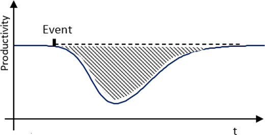
Figure 1 shows both the idealized course of a company’s productivity over time, assuming uninterrupted operations with a constant 100% productivity level, as well as a drop in productivity due to a disruptive event. The disruption occurs at a certain point in time and can be defined to last until productivity returns to its original level or higher. The shaded area in Figure 1 represents the resulting productivity loss.

To quantify this loss, we propose a mathematical model using two components:

1. a disruption function $D$⁠, which causes losses in the normal course of production; and

2. a recovery function $R$⁠, which describes the return to the initial productivity after the interruption.

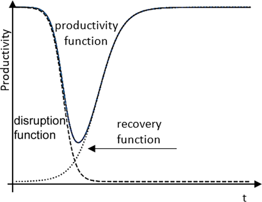
The two functions are represented by two sigmoidal curves, as shown in Figure 2. By adding and superimposing the sigmoidal curves of disruption and recovery, we obtain the desired productivity curve (Figure 3), which approximates the output function for the productivity shown in Figure 1.

Analogous to Cimellaro et al., we want to calculate the area of lost productivity (Cimellaro et al., 2010). However, we deviate from their approach in that we consider a new parameterization using the disruption and recovery functions.

We define $Dt,TOE,TRE$ with $0≤D≤1$ as the curve of the disruption over time $t$ given an event that occurred at time $TOE$ before countermeasures were taken and recovery began. The steepness and position of $D$ describes how strong the impact of the disruption is. For example, a scenario can occur in which the decrease of an interruption is so strong that productivity drops to zero. In this case, an even stronger recovery is required to boost productivity back to 100% in a timely manner.

We define a recovery function $Rt,TOE,TRE$with $0≤R≤1$⁠, which works against the reduced productivity and leads to a time-dependent recovery of productivity. $TRE$ describes the time at which productivity is fully restored. To limit the calculation to the time interval of the event, the Heaviside step function $H(t)$ is used, where $Ht=1$ if $t≥0$ and $Ht=0$ if $t<0$⁠. The resulting superimposed curve can therefore be described as:

where $Q(t)$ represents the total productivity at time t. It combines the disruption and recovery function and is derived from the superposition of sigmoidal curves. The functions $Q$⁠, $D$ and $R$ depend on a supply network (⁠$SN$⁠) and correspond to a single event $e$⁠, but we omit the dependency in the mathematical derivations for readability. To calculate the strength of the impact of a disruption, i.e. the loss, on a supply network $SN$ over the time of an event $e$⁠, we take the integral of $Q(t)$ over time:

Risks are always viewed as a loss, i.e. a given extent of damage, with a certain probability of occurrence. Here we assume that an event $e$ causes a disruption that leads to an interruption and thus causes a loss in a supply network $SN$ and therefore represents a risk. To calculate the risk $R SN| e)$of event e, we use the definition given by March and Shapira of risk as the product of the loss of the event $LSN|e)$ and its probability $P(e)$ (March and Shapira, 1987):

Using the approach of Cox (Cox, 2008), the probability of a risk can be calculated as the product of a threat $T(e)$and the firm’s vulnerability to that threat, $V(e)$⁠. Here, a threat is an event likely to cause an impact. Vulnerability, as explained in Section 2.1, is any weakness in a system that can be exploited. Assessing the vulnerability of a supply network to an event can be difficult. However, vulnerability can also be formulated differently, namely, as the robustness of the system after an event. We say a supply network is robust if an event has no impact on supply delivery. If an event has an impact on a delivery network, productivity drops and the delivery network is vulnerable. It follows that robustness and vulnerability are inversely proportional.

Finally, following Cox, the threats and vulnerabilities are multiplied by their loss functions to obtain the risk. With direct and indirect losses given by $L(e)$⁠, we arrive at the following formula:

To calculate the overall risk to a supply network, let Events be the set of all known events that could affect a company’s productivity. These are accumulated into a total network risk $SNR$⁠:

The overall risk can be used to check whether targeted measures towards an event can reduce the associated risk in a supply network without increasing the risk exposure to other events. This comprehensive calculation is more time-consuming, the more events are considered, but it enables an accurate assessment of the expected performance of a supply network configuration.

This mathematical approach provides a framework to assess vulnerabilities and their risks. It allows for optimizing a supply network by making adjustments to find a configuration that minimizes the total risk a company is exposed to given a set of possible events.

If measures are implemented in a supply network to restore full productivity quickly after an interruption, and options are set up to support the adaptability of supply networks, we speak of balanced resilience.

This emphasizes that risk, adaptability and resilience are inextricably linked, and it is their balance that determines supply chain resilience. Looking at the magnitude of an event’s risk, we can prioritize targeted measures for high-risk events over other measures. However, the risk magnitude itself does not give us any information on how to mitigate the risk most effectively given a certain event. To tackle this challenge, we close the gap between risk calculation and quantification of resilience indicators, which we derive from the disruption and recovery functions (Figure 3) in the following section. To demonstrate the applicability of the proposed mathematical framework, we apply it to a stylized simulation in the subsequent section. This simulation serves as an illustrative example for evaluating the productivity impact of disruptions and testing selected resilience strategies.

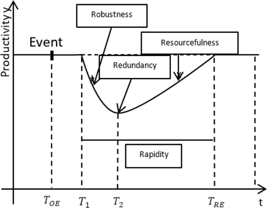
Balanced resilience can be expressed through four Rs of resilience to improve skills and resources. We propose a new mathematical derivation for the so-called four Rs of resilience, i.e. robustness, resourcefulness, redundancy and rapidity, such that each can be quantified and compared against other network configurations. For this purpose, we improve the approach of Cimellaro et al., who calculated earthquake disaster resilience (Cimellaro et al., 2010) and make it applicable to supply chain risk management, as illustrated in Figure 4. Based on this, the four Rs of resilience can be quantified as follows:

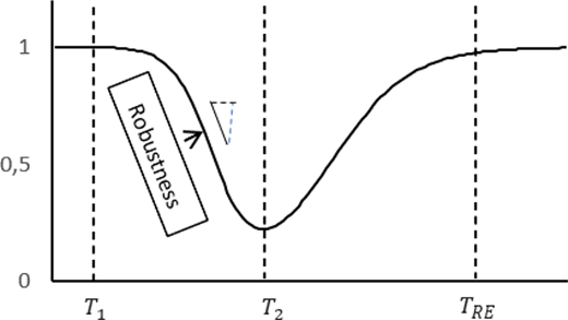
Robustness (Figure 4) is the ability of a system to withstand loads and stressful events while minimizing disruption (Bruneau et al., 2003; Minsker et al., 2015). The robustness of a system is directly proportional to its capacity to absorb initial disturbances, thereby enhancing its ability to withstand shock events and preventing an immediate decline of productivity. Consequently, the system’s robustness is manifested in the position of the inflection point of the disruption curve $D$ and its decline thereat. We argue that the weaker the decline and the later the disruption starts, the more robust a supply network is. Thus, Robustness is optimal if the slope divided by the time passed since the start of an event until the curve reaches its inflection point is minimal. This can be expressed mathematically as:

In the context of supply networks, it should be considered that productivity does not usually fall immediately after the occurrence of a shock event. Fischäder refers to the period between the occurrence of an event and the occurrence of interruptions as the buffer period (Schneider and Haupt, 2007). In mathematical terms, it is desirable if this duration is maximum, i.e. if $T1→TRE$⁠, as this reduces the loss of productivity with the optimal case being $T1=TRE$⁠.

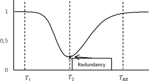
Redundancy (Figure 5) includes the ability to quickly switch to alternative resources (i.e. suppliers or materials) if the main resources are insufficient. It depends on the substitutability (Minsker et al., 2015). The rate at which the transition to an alternative resource occurs determines the point where the recovery curve $r$ overtakes the disruption curve $d$⁠. Consequently, we utilize the intersection of the two s-curves since at this point, the loss of productivity is maximal and the recovery starts to kick in. This indicator of redundancy can be utilized to assess the magnitude of the disruption; the more effectively the disruption is mitigated, the more favourable the outcome. Thus, redundancy is at its optimum if the following formula is minimal:

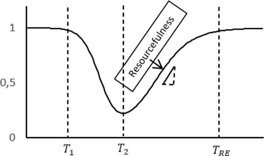
Resourcefulness (Figure 6) is the ability to identify problems, prioritize them and mobilize resources in response to disruptive elements (Bruneau et al., 2003). This is the rate and timespan at which the productivity returns to its original level. It quantifies how quickly countermeasures can be initiated, i.e. how flexibly the supply chain can adapt to stop the decline and return to the initial level, in other words, to recover. It corresponds to the position of the inflection point of the recovery curve, relative to the event start and its slope thereat. Resourcefulness is thus the counterpart of robustness and is at its optimum if the following formula is minimal:

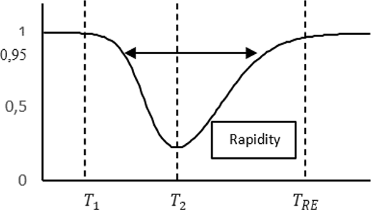
Rapidity (Figure 7) indicates how quickly the initial productivity can be reached again after the shock event (Minsker et al., 2015). The shorter this period, the better the loss can be limited. To quantify rapidity, the time passing between where the disruption starts, until the recovery is achieved, can be used. We suggest using the 95% disruption and recovery to mathematically represent the rapidity as:

We can see how closely Rapidity, Resourcefulness and Redundancy are linked and depend on each other. The more substitutes are available and the faster a company can access them, the shorter the time to return to the initial level. Rapidity, Resourcefulness and Redundancy therefore have a direct effect on the productivity function from Section 3.1. The more resilient the measures incorporated into a supply network, the more flexible that network is against disruptive events. This framework provides a better understanding of what and how measures can have a positive impact on a company’s productivity. We will demonstrate this localization in the next chapter using a simple case study based on a simulated supply network.

In the following section, the proposed mathematical framework is applied within a simplified simulation environment to illustrate its practical relevance. Rather than replicating a real-world case study, which would require extensive company-specific data, behavioural calibration and digital twin-level modelling, we demonstrate the conceptual functionality of the model through a stylized example and thus pave the way for future research on this matter. As such, this approach is consistent with resilience modelling practices that advocate simulation-based exploration before empirical implementation (Bruneau et al., 2003; Vugrin et al., 2010). It also reflects recent calls in the literature for transparent methodological foundations as a prerequisite to data-driven validation (Bruckler et al., 2024; Cimellaro et al., 2010; Ivanov, 2023b).

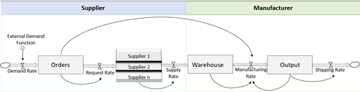
The SD model simulates a company’s simplified supply chain to illustrate how the system behaves in disruptive scenarios. The model relies on several assumed parameters (see  Appendix 2), carefully selected to reflect stylized yet plausible supply chain dynamics. Figure 8 illustrates the stock-and-flow diagram of the supply chain model. The box elements represent stocks (e.g. levels of orders, warehouse inventories), while flows are illustrated as triangular valves.

In the model, customer orders are generated based on a sinusoidally increasing rate and introduced as system demand. Production depends on the available warehouse inventory and is constrained by a maximum production capacity. As a result, orders are processed dynamically through the system. If a single source of supply is used, the company relies solely on that supplier, producing according to incoming orders and production limits. Finished goods are then transferred from supplier to company warehouse, which acts as a buffer or operates at minimal levels in just-in-time setups. The employee’s flexibility can be modulated and influences how quickly production can adjust to changing targets, with lower flexibility leading to longer adjustment time. All simulation parameters and their contextual interpretations are documented in  Appendix 2 to ensure a transparent assessment of the resilience measures applied and replicability of the results. Table A3 in  Appendix 2 presents the definition and assumptions for each parameter, including their operational interpretation.

The simulation aims to evaluate how selected resilience measures can influence supply chain recovery after a disruption. We define the company’s productivity as the rate of successfully fulfilled orders over time with:

As such, if the shipping rate corresponds to the demand rate, we assume ideal productivity. Therefore, any delays in production or material supply can lead to shipment delays and thus reduced productivity.

To demonstrate the impact of the disruption and the effectiveness of different mitigation strategies, a variety of scenarios are modelled without any resilience strategies and with the application of three specific strategies, buffer stock, dual sourcing and workforce flexibility, which are parameterized as follows:

1. For the buffer stock measure, inventory is increased from 0 to 10 units (refer to parameters in  Appendix 2).

2. In the dual sourcing scenario, an additional supplier covers 30% of orders.

3. To simulate employee flexibility, the parameter was adjusted from 0.1 (indicating no flexibility) to 0.9, representing full flexibility.

4. No resilience measures are applied (baseline).

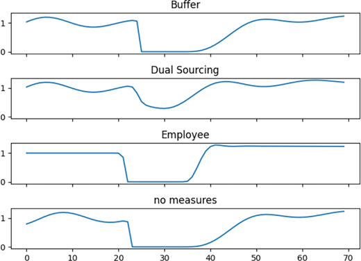
Figure 9 shows the resulting productivity curves, where a disruption is introduced at time step 100 in the form of a 15-day shortage of input material.

The four scenarios demonstrate distinct recovery behaviours, which are evaluated in terms of total production loss and associated risk. To evaluate the risk of an event, the related productivity loss is quantified in terms of lost production days. This is calculated as the integral under the productivity curve, assuming an idealized 100% productivity level. In the subsequent step, this loss is multiplied by the disruption probability to assess the associated risk. For illustrative purposes, a winter storm scenario with a 60% probability of occurrence (World Economic Forum, 2023) is assumed. Table 1 presents the evaluation of lost production days as well as the associated risk, which can subsequently be used to compare the magnitude of various events to variations in the supply network.

All examined measures reduce production loss to varying degrees, with dual sourcing showing the strongest effect. These patterns are analyzed in more detail in Table 2. Without mitigation, a 15-day disruption result in approximately 19 lost production days. By contrast, with a buffer stock of ten stored material units, the loss is reduced to approximately 16 days, as the production rate consists of approximately three items per day. The calculated risk serves as a reference point for comparing disruptions of varying likelihood.

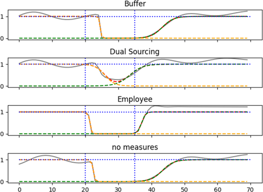
With the productivity curve, we can also compute both the disruption and recovery functions and the four Rs of resilience, which can give more insights into how resilience strategies can improve the productivity. This involves several steps: firstly, the productivity curve is decomposed into disruption and recovery components using sigmoidal functions. For this, we use the generalized logistic curve with the given mathematical formulation as follows:

The calculation could alternatively be conducted using other curves, such as the Gompertz curve ( Appendix 1). In this function, $a$ represents the limit value. We assume a limit value of $a=1$ to constrain the curve to 100% productivity. $b$represents the maximum slope and $c$ the temporal shift of the inflection point. The vertical offset $d$ is not relevant in this context, as the end point is $0$ and is therefore omitted.

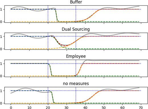
We use an optimization routine to iteratively adjust the parameters, so the resulting superposition fits the original productivity curve. Figure 10 presents the two Sigmoid curves (green and yellow) alongside the initial productivity curve (grey). For comparison, the corresponding results for the Gompertz curve are reported in  Appendix 1 (Figure A1), and the associated loss analysis in production days as well as its evaluation are summarized in  Appendix 1 (Table A1 and Table A2).

With the fitted sigmoidal curves at hand, we can now calculate the four Rs of resilience using the parameters $b$ and $c$⁠. Robustness uses the value of the maximal slope and the inflection point of the disruption curve, which for the logistic function are given by $-bd4$ and $cd$⁠. Redundancy is calculated using the value of $Q(t)$ at the intersection point. Resourcefulness is the counterpart of the Robustness, which is why it uses the slope and inflection point of the recovery function. We divide the resourcefulness by 1,000 for readability. Lastly, rapidity measures the duration of the interruption, i.e. the time until the recovery reaches 95% after the disruption first dropped below 95%. Thus, the mathematical formulations of the four Rs or resilience are:

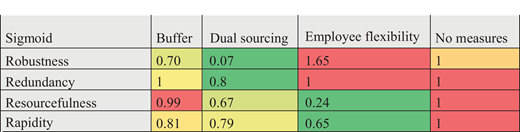
Table 2 presents a comparison of the resilience measures given the supply chain variations under the simulated event. The best values are highlighted in green, whereas the least favourable values are marked in red.

For robustness as well as redundancy, dual sourcing demonstrates the most effective outcome. These results suggest that dual sourcing primarily influences the disruption curve, whereas employee flexibility has a greater impact on the recovery curve. Buffer stock exhibits the least overall effect. However, it shows an improvement in Robustness even with the small change from a buffer stock of ten materials. We evaluated that upgrading to a buffer stock of 20 materials, the loss can even be reduced from 0.704 to 0.395.

These findings confirm previous observations in the literature while extending them through quantitative validation. For instance, Bruckler et al. emphasize the trade-offs associated with inventory-based resilience strategies, which our results support by showing the limited standalone effect of buffer stock (Bruckler et al., 2024). Similarly, Aldrighetti et al. highlight dual sourcing as a high-impact resilience investment a finding mirrored in our model, where this strategy shows the strongest effect on both robustness and total loss reduction (Aldrighetti et al., 2023). In contrast to approaches like Li et al. and Poornikoo and Qureshi, which simulate disruption dynamics without explicitly linking them to loss quantification, our framework allows direct evaluation of the economic effectiveness of specific strategies (Li et al., 2021; Poornikoo and Qureshi, 2019). This bridges the gap between theoretical resilience metrics and practical decision-making tools.

The proposed framework integrates risk and resilience assessments and offers a structured approach to evaluate the resilience of supply networks. By linking resilience indicators to productivity losses, organizations can compare the effectiveness of different strategies. These indicators and the associated loss in production days serve as a basis for prioritizing targeted measures and aligning them with risk exposure. Furthermore, through decomposing productivity into disruption and recovery functions, companies can apply the model using internal performance data to derive key resilience metrics. This enables both scenario-based planning and dynamic resilience monitoring. As such, this approach allows companies to proactively evaluate potential disruptions and optimize their strategic response by approximating their supply network with a system dynamics simulation model.

Simulations provide a framework for assessing the economic significance of disruption events and thus reducing ambiguity in resilience analysis. However, inaccurate determination of the relevant shock events and inadequate estimation of the probabilities of occurrence for various events can impair the effectiveness of the calculations. Given the complexity and uncertainty of real-world risks, exact probabilities of disruptive events are often difficult to estimate. These can be collected, for example, from World Economic Forum reports or by means of surveys (World Economic Forum, 2023). By simulating a wide range of potential disruptions and their associated risks, this approach can provide more comprehensive insights into supply chain vulnerabilities and enable optimization of resilience. Thus, simulation offers a good solution to explore various scenarios in a risk-free manner and to identify measures to strengthen supply chain resilience.

Moreover, the framework provides a structured basis that paves the way for evaluating trade-offs between cost and resilience. By translating productivity losses into monetary terms, managers can estimate the potential economic value of resilience investments and identify strategies that offer a favourable balance between additional cost and risk reduction. This quantitative view helps to advance resilience from a qualitative concept toward a decision-oriented and financially interpretable metric.

Realizing these insights in practice requires the development of models that can reflect actual supply chain configurations and their interdependencies. A validation of the risk-loss function and resilience indicators using a real-world company model is thus an open challenge for future research. Future work should thus focus on expanding the practical application and on how to adapt the simulated supply chain to represent the complexity and accuracy of the real world. While the current study demonstrates the applicability of the framework using a stylized simulation, the integration into a real-world scenario and applying the model to empirical company data would require detailed mapping of supplier networks, lead times, event probabilities and system-specific behaviour, an effort resembling the development of a digital twin and extending beyond the scope of this methodological contribution.

Nonetheless, the proposed framework already offers decision-makers a structured method to quantify and compare the effects of resilience strategies. By translating productivity losses into risk-adjusted performance indicators, the model supports scenario testing and evidence-based investment planning. To deliver tailored guidance for specific supply chain configurations, future research should focus on the empirical calibration of the risk loss function and resilience indicators using historical productivity and disruption data.

This study developed a mathematical framework to quantitatively assess supply chain risk and resilience through an integrated system dynamics approach. By combining risk modelling and resilience metrics within a unified structure, the framework enables a transparent quantification of productivity losses and provides a consistent basis for evaluating resilience-enhancing measures. The simulation results demonstrated how different strategies, such as buffer stock, dual sourcing and workforce flexibility affect disruption recovery and overall supply chain performance.

The proposed framework contributes to the growing body of resilience research by offering a mathematical formulation that connects risk exposure and resilience performance. In contrast to qualitative or scenario-based assessments, the approach translates resilience into measurable, risk-adjusted indicators and thereby supports the operationalization of resilience in quantitative modelling and simulation studies.

From a managerial perspective, the framework provides a structured basis for comparing the economic effectiveness of resilience strategies. By translating productivity losses into monetary terms, decision-makers can evaluate trade-offs between cost and resilience and identify measures with the highest marginal benefit in reducing expected losses. This enables a more transparent and data-driven approach to prioritizing resilience investments across alternative strategies and scenarios.

While this study focused on a stylized simulation environment, future research should extend the framework to multi-tier and empirically calibrated supply chains. Integrating stochastic demand patterns, correlated risk events and multiple simultaneous disruptions would further enhance its applicability. Moreover, coupling the model with real-world data or digital twin applications could provide stronger empirical validation and managerial usability.

$Gompertz curve = ae(-be)(-ct)+d, where a=-1 and d=1.$

The resulting formulas of the resilience indicators are:

We can see that depending on the function used, the results do not differ significantly.

The following table provides an overview of the parameter settings used in the simulation model, including a brief explanation of their role and interpretation within the supply chain context.