Beyond technology: how systemic coordination enables AI integration in manufacturing

Previous studies often treat the integration of AI in manufacturing as either a technical modeling task or an organizational change task. This study challenges this separation. In a nine-month case study at a heavy-duty vehicle manufacturer, we found that technical development and organizational adaptation are fundamentally interdependent and cannot be sequenced. Interdependencies between model performance, equipment control, and maintenance coordination emerged that no upfront plan could fully anticipate, but were essential to train and validate the model and make its output usable in practice. The resulting AI model achieved 12–37% better anomaly detection than traditional methods, with the largest gains on subtle defects.

This study introduces the concept of “systemic coordination” as a defining characteristic of AI integration, where technical and organizational changes only become visible during integration itself. We extend socio-technical systems theory by showing how interdependencies emerge dynamically and by developing dual iterative learning cycles that coordinate technical development and organizational adaptation.

Treating AI as a “build first and deploy later” project risks failure regardless of model quality. Manufacturing companies should conduct parallel technical and organizational activities using dual iterative learning cycles, supported by cross-functional workshops, feedback loops, physics-based validation, and customized interfaces for operators, maintenance, quality and engineering teams.

Production systems generate large amounts of data but despite much progress in data analytics adoption, manufacturing companies still rely heavily on manual methods for quality control (Fragapane et al., 2023), limiting the potential of data-driven insights and proactive quality control. To remain competitive, manufacturing companies must adopt automated data processing methods (ElMaraghy et al., 2021).

Traditional Statistical Process Control (SPC) methods (Shewhart, 1931; Montgomery, 2017) face significant limitations in detecting subtle deviations in complex multivariate data (Chu et al., 2024). This is particularly true when high-mix production and dynamic testing conditions create non-linear patterns that exceed the capabilities of established statistical techniques (Chhetri, 2024).

AI-based anomaly detection addresses these limitations by adapting to changing data distributions and learning complex patterns from operational data (Chhetri, 2024). Through real-time data collection and analysis, AI systems provide consistent process monitoring, enabling early detection of emerging issues and supporting higher quality control standards (Fährmann et al., 2024; Leberruyer et al., 2023).

Despite these advantages, the adoption of AI-based systems in the manufacturing sector remains heterogeneous and far from universal. First, it faces significant technical challenges such as manual feature engineering, imbalanced datasets, and limited model interpretability (Ismail et al., 2020; Xie et al., 2025; Elía and Pagola, 2025; Moosavi et al., 2024). Variational Autoencoders (VAEs) can address these gaps by learning patterns from nominal data to quantify deviations (Kim and Kim, 2023; Hiranaka and Tsujino, 2024). However, most studies remain at the proof-of-concept stage. The challenge is moving beyond local applications to system-level integration, where AI is embedded into multi-stage decision-making workflows (Arinez et al., 2020; Bokrantz et al., 2024).

Technical performance alone does not guarantee successful AI integration. Unlike conventional manufacturing technologies available as off-the-shelf solutions, AI requires extensive customization and continuous adaptation (Arinez et al., 2020; Plathottam et al., 2023; Peretz-Andersson et al., 2024). These challenges highlight that successful AI integration is not merely a technical exercise but a transformation that requires systemic coordination to prevent technical silos. Because AI performance is sensitive to physical process changes, there is an acute need for coordination between those managing the algorithm and those managing the production hardware to ensure long-term model reliability (Powell, 2024).

Existing frameworks address technical development and organizational adaptation separately, leaving critical gaps. While implementation often treats AI as a sequential technical activity followed by organizational deployment, this study examines integration as a process of systemic coordination. This approach recognizes that AI technology cannot be developed apart from the organizational context, requiring a coordinated development where technical design and organizational adaptation are adjusted in response to one another.

Recent work recognizes that AI requires developing technical and organizational capabilities together, but provides limited guidance on managing this coordination during development.

Therefore, this study analyzes how technical development and organizational adaptation are coordinated during AI integration in manufacturing quality control. A nine-month case study was conducted at a heavy-duty vehicle manufacturing company facing transmission noise challenges caused by subtle manufacturing deviations. A VAE model was developed and validated using quantitative metrics for performance analysis and qualitative stakeholder feedback. The study focuses on the development and initial deployment phase, examining how coordination during this period builds capabilities for sustained AI integration.

This study makes three interconnected contributions. First, we demonstrate that AI development creates systemic coordination requirements where technical and organizational dimensions are interdependent and cannot be sequenced; this approach addresses the need for systemic coordination between departments. Second, we introduce dual Plan-Do-Check-Act (PDCA) cycles for coordinating technical development and organizational adaptation; this mechanism bridges the gap between technical frameworks (CRISP-DM, MLOps) and organizational frameworks (TOE, DOI). Third, we identify human-AI interface design principles: graduated severity scoring, familiar visualizations, and multi-layered explainability. These principles show that preserving human agency requires joint consideration during development, not post-hoc adjustments.

For this study, we examine AI integration within the context of anomaly detection in manufacturing quality control. This technical context presents specific coordination challenges that help to identify integration dynamics applicable to broader AI applications.

As manufacturing processes grow in complexity, traditional quality control methods, like those initiated by Shewhart and Taguchi, face significant limitations with today's high-mix and high-precision demands (Shewhart, 1931; Montgomery, 2017; Taguchi et al., 2005). While statistical outlier methods provide a foundational framework (Hawkins, 1980; Barnett and Lewis, 1994), they struggle to identify subtle deviations from process drift or unexpected events. This is particularly noticeable in industries like automotive and aerospace, where products are tested under dynamic conditions and generate complex multivariate signals (Chu et al., 2024).

AI-based anomaly detection addresses this gap by analyzing complex inter-dependencies in multivariate data more easily than statistical methods (Zeiser et al., 2023). This method can identify subtle deviations before they become failures, as demonstrated in semiconductor production, machine tool monitoring, and component inspection (Gorman et al., 2022; Pota et al., 2023; Liu et al., 2023).

However, implementing AI-based anomaly detection faces three critical technical challenges. First, transforming raw signals into meaningful features is laborious and depends on expert domain knowledge. Traditional methods rely on handcrafted features such as RMS, kurtosis, or peak-to-peak amplitude selected based on expert knowledge to simplify data before model training. However, this process is highly dependent on engineers’ expertise and can be ineffective for subtle or previously unseen defect types, as relevant features may be unknown in advance, leading to crucial information being discarded (Ismail et al., 2020; Li et al., 2018). This challenge is made more difficult by skill gaps between defect physics domain experts and feature extraction data scientists.

Second, defect rates below 1% create highly imbalanced datasets (Xie et al., 2025). Although many anomaly detection models can learn from normal data, they still require some anomaly examples for performance evaluation and threshold selection. Researchers have explored generating synthetic data through techniques including noise addition, Synthetic Minority Over-sampling Technique (SMOTE), and generative AI models (Fernández et al., 2018; Niu et al., 2020). However, synthetic defects often fail to capture intricate physical characteristics of real-world defects, leading to models narrowly focused on synthetic patterns that prove less effective in actual production (Ekwaro-Osire et al., 2025).

Third, many AI models operate as “black boxes” that cannot explain their predictions, creating significant acceptance barriers. Trust often precedes technical performance in AI adoption (Xiong et al., 2024). Quality engineers need to understand the reasoning behind anomaly predictions before disrupting production. While post-hoc explanation methods provide insights after the model is trained, they rely on engineered features whose relevance to defect characteristics is not guaranteed in advance.

This challenge is particularly pronounced in vibration-based gear monitoring, where subtle defect indicators have various causes, making detailed reasoning from the AI model essential but difficult to obtain (Chu et al., 2024; Moosavi et al., 2024; Elía and Pagola, 2025; Gorman et al., 2022).

VAEs address these challenges by learning complex patterns from nominal data and quantifying deviations (Kim and Kim, 2023; Hiranaka and Tsujino, 2024). A VAE is a type of neural network consisting of two components: an encoder that compresses normal operational data into a lower-dimensional latent representation, and a decoder that attempts to reconstruct the original data from this compressed form. During training, the VAE learns what “normal” looks like by minimizing reconstruction error on nominal samples. When presented with new data, larger reconstruction errors indicate deviations from learned normal patterns, serving as anomaly indicators (Kingma and Welling, 2013). This architecture directly addresses the three technical challenges previously identified.

First, automatic feature discovery eliminates the need for manual preprocessing and handcrafted features (Ismail et al., 2020). Second, training exclusively on normal data handles imbalanced datasets without requiring defect examples for model development (Kim and Kim, 2023). Third, the interpretable latent space addresses the black-box problem by providing uncertainty quantification while revealing meaningful patterns that quality engineers can examine (Usmani et al., 2024; Jakubowski et al., 2021; Elía and Pagola, 2025; Ghobakhloo et al., 2024).

While standard autoencoders address feature engineering and imbalanced datasets, VAEs provide additional capabilities critical for manufacturing integration. The probabilistic latent space enables uncertainty quantification, helping quality engineers assess confidence in anomaly scores (Usmani et al., 2024). The regularized latent space creates an interpretable structure where similar products cluster naturally, supporting root cause investigation (Elía and Pagola, 2025). Finally, the generative capability enables synthetic sample creation for validation testing when real defect data are scarce (Kim and Kim, 2023). These VAE-specific characteristics address both technical performance requirements and organizational acceptance challenges in manufacturing environments.

Despite these technical advantages, VAEs are not widely used in manufacturing, and questions remain about their integration in real-world quality control applications (Elía and Pagola, 2025; Jakubowski et al., 2021). These questions extend beyond technical performance to include organizational challenges.

Unlike traditional manufacturing technologies available as off-the-shelf solutions, AI cannot simply be purchased and directly integrated into existing systems (Chatterjee et al., 2021; Maroufkhani et al., 2023). AI requires extensive customization and continuous adaptation, creating distinctive coordination requirements during deployment.

AI integration extends socio-technical systems (STS) theory, shifting focus from local technical implementation to the systemic coordination of organizational change (Makarius et al., 2020; Benbya et al., 2021). However, literature often uses “implementation” and “integration” interchangeably. We distinguish these terms based on temporal and systemic requirements. Traditional technology implementation follows sequential development then deployment, while AI integration requires parallel technical design and organizational adaptation through active coordination (Cherns, 1976; Baxter and Sommerville, 2011). This operationalizes STS theory's joint optimization principle (Pasmore et al., 1982). Table 1 summarizes this distinction.

STS theory (Trist and Bamforth, 1951) emphasizes that effective organizational systems emerge from the alignment of technical capabilities with social structures and human needs. The “social” subsystem includes people, their relationships, organizational culture, values, communication patterns, and work-related processes and structures. The “technical” subsystem includes tools, technology, processes, and methods. This theory recognizes that optimizing one subsystem at the expense of the other leads to overall degradation. Instead, it recommends that both are designed and managed through mutual adjustment for optimal system performance (Cherns, 1976).

Beyond technical performance, integration requires fundamental workflow changes, raising questions about decision authority and organizational resistance. Manufacturing companies must manage three distinctive changes during AI integration: working with probabilistic outputs rather than deterministic rules (Maged and Xie, 2022), establishing collaboration between manufacturing engineers and AI specialists to encode domain knowledge (Cannas et al., 2024), and maintaining continuous model updates as production conditions evolve (Arinez et al., 2020; Plathottam et al., 2023). These changes require proper change management practices such as training, communication, and participatory design. Without these practices, integration efforts fail due to inadequate workflow integration, insufficient data infrastructure, or organizational resistance due to limited AI understanding (Peretz-Andersson et al., 2024; Arinez et al., 2020; Chu et al., 2024; Elía and Pagola, 2025).

While technical frameworks, such as Cross-industry standard process for data mining (CRISP-DM) or Machine Learning Operations (MLOps) guide data science workflows (Wirth and Hipp, 2000; Kreuzberger et al., 2023) and organizational frameworks, such as Technology-Organization-Environment (TOE) or Diffusion of Innovation (DOI) explain adoption factors (Tornatzky et al., 1990; Rogers, 2003), these frameworks address technical development and organizational adoption separately. Technical frameworks provide structured processes for AI model development but offer limited guidance on organizational integration. In contrast, organizational frameworks explain what factors influence adoption decisions but not how to manage the integration process itself (Peretz-Andersson et al., 2024).

Makarius et al. (2020) demonstrate that AI integration requires building organizational capabilities that enable employees and AI systems to collaborate effectively. Benbya et al. (2021) highlight that AI systems are embedded in broader sociotechnical contexts where social factors shape how AI works and what value it creates. These social factors include organizational practices, human capabilities, and institutional norms.

However, while STS theory identifies the need for parallel technical and organizational adaptation, it provides limited guidance on the operational mechanisms for managing the temporal coordination of these parallel processes during integration (Peretz-Andersson et al., 2024). This gap is particularly significant in manufacturing contexts where production stability requirements create tension with AI's need for experimentation and iteration.

This creates a critical gap: existing research either optimizes technical performance assuming organizational factors can be addressed later, or examines organizational adoption treating technical systems as fixed. How technical design and organizational adaptation can be coordinated during development remains unclear.

This study analyzes how systemic coordination is achieved during AI integration in manufacturing quality control. Given that AI integration is not a simple linear event but a multifaceted socio-technical process, we adopted a single case study design (Yin, 2018) to provide a deep, contextual, and longitudinal understanding of the complex interplay between technical development and organizational dynamics. Case study methodology has proven successful for investigating AI integration in manufacturing, where the complexity of integration processes requires detailed longitudinal observation that survey-based or experimental methods cannot provide (Peretz-Andersson et al., 2024; Bokrantz et al., 2024).

The research was conducted within a Collaborative Management Research (CMR) framework, where researchers and practitioners acted as co-investigators (Shani et al., 2008). This approach was essential because integrating AI required bridging the gap between advanced theory and the practical realities of the organization (Rami Shani et al., 2012). As an insider researcher, the lead author gained access to both formal data (measurements, documents) and informal data (daily observations, spontaneous discussions) over the nine-month period, facilitating trust-building and a deeper understanding of the organizational context (Shani et al., 2008; Rami Shani et al., 2012).

The case company was a heavy-duty vehicle manufacturer facing persistent transmission noise issues affecting a few axles but creating significant rework costs. With the industry's shift to quieter electric powertrains, resolving these noise issues became a critical business priority.

This case represents a critical case (Yin, 2018) where conventional quality improvement methods had failed. Despite extensive verification steps along the manufacturing line and inconclusive studies examining correlations between axle vibration levels and vehicle noise, the company could only mitigate the problem, never eliminate it completely. Design of Experiments was economically unfeasible given low production volumes and high product variety, while manual inspection lacked the sensitivity to detect subtle defects. Redesigning the powertrain was not economically justified given the issue's low frequency. This sustained failure created an opportunity where integration challenges became more visible than in contexts with multiple viable solution paths, making it an ideal environment to explore the nuanced challenges and success factors of integrating a novel AI solution. The case met key enabling conditions: availability of relevant sensor data, low defect rates, significant rework costs, cross-functional involvement that includes assembly, quality, maintenance, IT, and engineering, and an established continuous improvement culture.

While the findings of this study are based on a single case study, the research leverages a rich set of real-world operational data. This provides robust information on AI integration in manufacturing environments, enhancing the relevance and transferability of results. Importantly, the study goes beyond a purely technological perspective by considering organizational and process-related factors that influence successful AI integration in real-world production settings.

The integration followed an iterative Plan-Do-Check-Act (PDCA) cycle, a continuous improvement methodology routinely used by the company. Workshops followed the Check-Act-Plan pattern, reviewing progress, deciding corrective actions, and allocating responsibilities. The Do phase occurred between workshops as teams executed plans. Changes affecting only specific functions were managed through bilateral discussions, with outcomes communicated to other stakeholders.

The first workshop was initiated by management to address transmission noise issues affecting less than 1% of axles but representing significant waste. The goal was to integrate quality control at the cleaning cell of transmission axles where vibrations are measured while the axle’s shaft is rotated. Two parallel methods were decided: a conventional RMS-based threshold and an AI-based anomaly detection system. Given the unknown mechanism causing noise propagation and difficulty identifying relevant features for traditional machine learning, a neural network model was selected, with VAE chosen over standard autoencoders for its ability to generate synthetic samples and manipulate the latent space for model validation.

Initial analysis revealed that brake control was insufficient to ensure proper repeatability. The first major activity optimized Programmable Logic Controller (PLC) parameters across five controllers, a four-month process constrained by maintenance scheduling (half-day sessions every two weeks). A Master axle was introduced for bi-weekly repeatability verification.

A second workshop was held to review PLC improvements. Planned next steps consisted of parallel activities that included VAE development (three months), defining spectrogram calculations from raw vibration data, test cycle corrections, user interface design, and introducing the Master + axle (increased torque to simulate defects).

A third workshop presented VAE and RMS comparison results. Planned outcomes established the phased threshold approach, and finalized deployment decisions.

This detailed process description illustrates how technical development activities and organizational coordination evolved in parallel, which is essential for understanding the sociotechnical dynamics of AI integration.

A custom dual-input VAE architecture was developed to simultaneously analyze time-series signals (rotation speed and torque) and vibration patterns. The architecture employs convolutional neural networks that encode mel-scale spectrograms of size 272 time steps by 256 frequency bins, reducing them to a 32 × 34 representation before entering a 16-dimensional latent space that captures essential vibration characteristics.

VAE development progressed through major architectural iterations, starting with an Artificial Neural Network before adopting a Convolutional Neural Network structure based on superior performance for pattern recognition in spectrograms. Multiple techniques for integrating time-series signals were tested. Model selection criteria combined quantitative performance metrics such as Mean Absolute Error (MAE) with qualitative visual assessment, prioritizing physically realistic reconstructed spectrograms showing plausible frequency patterns similar to originals.

The model was trained on approximately 500 axles using a standard 85/15 train-validation split, balanced across part numbers and test cells. Training optimized three loss components: MAE for both time-series and spectrogram reconstruction, as well as Kullback–Leibler divergence for latent space regularization.

For anomaly detection, the system uses MAE between original and reconstructed spectrograms as the anomaly criterion, where higher values indicate greater deviation from learned normal patterns.

The complete system was developed using Python with TensorFlow for the VAE model and Streamlit for the web-based user interface, with Claude 3.5 Sonnet supporting programming tasks.

The nine-month duration represented the initial integration phase: the system achieved function validation but limited production use.

Data collection was conducted over a nine-month period using a mixed-methods approach combining qualitative and quantitative data sources to ensure a comprehensive understanding of both technical performance and organizational dynamics during AI integration. Table 2 summarizes the data collection methods, sample sizes, and analytical purposes.

Qualitative data included semi-structured interviews, workshops, observations, and informal discussions.

Twenty semi-structured interviews were conducted with stakeholders representing diverse organizational functions: quality control (3), maintenance (2), manufacturing engineering (3), lean production (2), assembly operations (3), production management (2), information technology (3), and senior management (2). Participants were selected by purposive sampling based on their direct involvement in the quality issue under investigation or their operational responsibilities related to the transmission axle cleaning process. Interview duration ranged from 20 to 40 minutes, following a semi-structured interview guide organized around Rogers' five attributes of innovation adoption: relative advantage, compatibility, complexity, trialability, and observability (Rogers, 2003). This structure enabled systematic capture of stakeholders' experiences with AI integration while allowing flexibility to explore emergent themes and maintain consistency across interviews. Post-interview reflections were documented within 24 hours, and follow-up clarifications were conducted when necessary to ensure data integrity.

Three cross-functional workshops brought together stakeholders for structured problem-solving and solution design discussions. Each workshop followed a standardized agenda: (1) 20 minutes reviewing progress and identifying challenges, (2) 20 minutes discussing corrective actions and integration strategies, and (3) 20 minutes building consensus on next steps and responsibility allocation. Workshop sessions were documented through detailed notes by the lead researcher.

The lead researcher conducted observations and informal discussions by spending two days weekly at the manufacturing plant during the study period. This immersive presence facilitated the concurrent collection of formal data (via documentary analysis) and informal insights (via unstructured interviews with operators, engineers, and managers). Gemba walks were also used to understand the physical and social context of the production process.

Quantitative data consisted of testing measurements and operational performance metrics. Testing measurements included rotation speed, applied torque, and vibration data collected as axles rotated during the cleaning process. Two vibration sensors recorded data at 8,192 samples per second as each axle rotated in both forward and reverse directions during standardized 60-second test cycles. A total of 1,658 tests were used for model training. Raw vibration signals were processed into mel-scale spectrograms using Short-Time Fourier Transform, focusing on 50–1800 Hz where gear defects typically manifest.

For comparative analysis, Root Mean Square (RMS) values were calculated using traditional vibration analysis methods.

Additional quantitative data included production records, quality indicators and equipment maintenance data collected over six months to assess system performance.

Qualitative data were analyzed using thematic analysis (Braun and Clarke, 2006). The analysis process involved several iterative steps conducted manually by the research team. Initial open coding was performed on interview and workshop notes to identify preliminary concepts and patterns. These codes were then grouped into broader themes through constant comparative analysis. Emerging categories were continuously refined against new data.

Four main thematic categories emerged from this inductive process: understanding (how stakeholders comprehended the AI system), confidence (trust and acceptance levels), user experience (practical usability aspects), and integration enablers (factors enabling successful deployment). The analysis followed the principles of CMR, where interpretations were continuously validated through informal discussions with key practitioners to ensure alignment with operational reality (Shani et al., 2008). Hence, data collection and analysis proceeded iteratively until theoretical saturation was achieved, meaning no new insights emerged from additional data collection within the established categories. The themes identified represent stakeholder experiences during the initial deployment phase described in Section 3.2.1.

Quantitative analysis focused on comparing the performance of the AI model against the traditional Root Mean Square (RMS) vibration analysis method. The VAE model uses MAE between original and reconstructed spectrograms for both training optimization and operational anomaly detection score. Higher MAE values indicate greater deviation from learned normal patterns, suggesting potential anomalies.

The AI model performance evaluation used the Area Under the Receiver Operating Characteristic Curve (ROC AUC) metric, which measures the model's classification ability across different threshold settings. ROC AUC scores range from 0.5 (random performance) to 1.0 (perfect classification). To assess robustness, synthetic defects of varying severity levels were created using physics-based signal modifications, allowing controlled evaluation of detection sensitivity between different defect types and amplitudes. Model performance was evaluated on balanced datasets ranging from 768 to 1,568 samples.

The mixed-methods approach enabled triangulation between technical performance and organizational acceptance factors observed during integration. Qualitative data revealed how stakeholders' feedback shaped technical development: their needs for comprehensive visualization capabilities influenced system design, while concerns about visual interpretation informed model selection criteria toward physically realistic spectrograms that they could validate. Quantitative performance metrics were contextualized with qualitative observations, revealing whether technical results translated into practical value rather than representing technical excellence alone. This approach answered both the “can it work” (technical) and “will it be adopted” (organizational) questions, which is essential for evaluating AI integration.

Two techniques were tested to validate the AI model's ability to detect potential failures: physics-based signal modification and AI-based latent space manipulation. The physics-based technique proved to be the most valuable, allowing a direct comparison between traditional RMS-based anomaly criteria and AI-based reconstruction error on known failure modes with clearly understood characteristics. We attempted the AI-based technique, but it was not successful because of the VAE's inability to accurately reproduce measurement noise.

For the physics-based technique, vibration signals were altered through controlled perturbations in two ways: amplitude scaling (multiplying raw measurements by factors of 1.1x and 1.2x) and signal addition at frequencies corresponding to gear mesh frequency harmonics at different amplitudes (Table 3). These combinations were developed with company domain experts to create a realistic spectrum of issues from subtle early-stage defects to severe damage patterns, directly representing known failure mechanisms in transmission systems.

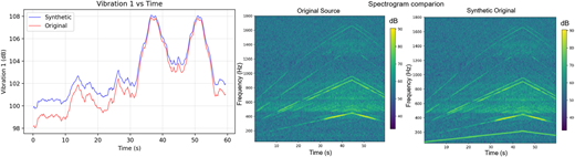
Figure 1 shows spectrograms when a signal at 0.5 times the gear mesh frequency was added with 0.08 m/s² amplitude, creating a high-severity defect visible in both RMS energy intensity and spectrogram patterns.

The VAE model was evaluated against the traditional RMS method on several synthetic physics-based defect severities. Using ROC AUC as the performance metric, each method was compared on identical balanced datasets ranging from 768 to 1568 samples. Balanced datasets contained equal numbers of normal and synthetic defect samples. Normal samples were randomly selected from the validation set, while defect samples were created by applying physics-based modifications (Table 3) to other samples from the validation set. Each baseline sample generated eight synthetic defect variants through different combinations of amplitude scaling and signal additions, enabling evaluation across multiple defect severities. To challenge the methods' detection capabilities, an additional set of defects was created using signal additions with amplitudes reduced by a factor of 10.

The VAE model outperformed the RMS method in all scenarios (Table 4), achieving ROC AUC scores of 0.881–0.941 versus 0.518 to 0.842 for RMS. The VAE model showed substantial performance advantages ranging from +12% to +37%, with the most pronounced improvements in challenging scenarios: amplitude reduction by a factor of 10 (+37%) and combined test cells datasets (+29%). First quartile (Q1) outperformed other statistical aggregations of the RMS signal.

The AI-based method demonstrated superior robustness by being less sensitive to equipment differences between test cells, which had different mounting configurations resulting in varying vibration amplitudes. The VAE model handled this without requiring equipment modifications, eliminating the need for costly individual standardization and calibration.

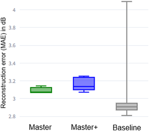
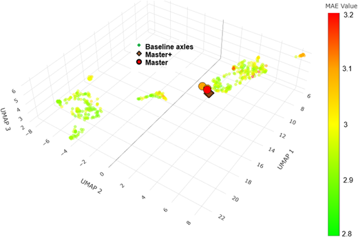
Initial deployment utilized a conservative operational threshold, to accommodate existing organizational constraints. This baseline calibration is intended to be iteratively refined, with plans to progressively tighten the detection boundaries (see Section 4.3.2). To further validate the system, an axle with a deliberately induced defect, called the “Master” axle, was dedicated for regular measurements to ensure repeatability. In addition, special test cycles called “Master+” were run. The Master + tests applied increased torque to create more severe vibrations, simulating worse defects. Torque readings were then normalized to standard test levels in post-processing, allowing the VAE to detect elevated vibrations under nominally normal operating conditions. Figure 2 shows reconstruction error (MAE) of the Master (normal test cycles), Master+ (increased torque cycles) and baseline axles (same size axles).

Both Master and Master + axles showed higher reconstruction errors than most baseline axles, confirming defect identification. All six Master + measurements clustered closely, demonstrating good repeatability. Baseline axles with errors above 3.5 dB resulted from testing issues rather than component defects.

Table 5 presents empirical evidence demonstrating how technical requirements and organizational adaptations were interdependent, requiring simultaneous coordination rather than sequential development.

These system-level interdependencies confirm AI is not a local add-on but a process-integrated capability. For example, achieving torque control required maintenance coordination, which influenced data collection timing, model training cycles, and ultimately stakeholder expectations.

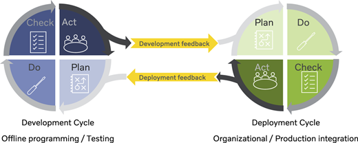
The core finding of this study is that AI integration requires systemic coordination, a process made possible by a dual PDCA framework that synchronized technical and organizational workstreams. The development cycle focused on offline technical work: VAE architecture development, synthetic defect validation, and user interface design. Simultaneously, the deployment cycle addressed organizational and process modifications: improving PLC control parameters, refining test protocols, and introducing the Master axle validation system.

Each cycle's outputs informed the other's planning phase through regular feedback loops, creating a coordination mechanism where technical and organizational dimensions progressed in parallel (Figure 3). This systemic approach was necessary because technical performance (model accuracy) was directly dependent on organizational stabilization (PLC control), demonstrating that these factors cannot be managed in isolation during AI integration. Master axle verification proves system-level integration, linking PLC control with AI.

This dual-cycle structure proved essential for managing AI's distinctive coordination requirements. User feedback on interface usability (deployment cycle) directly informed VAE presentation choices (development cycle), while synthetic defect validation results (development cycle) shaped stakeholder confidence and willingness to modify production processes (deployment cycle). When changes affected only specific functions, PDCA cycles were completed through bilateral discussions between relevant stakeholders, with other functions informed of outcomes, demonstrating the framework's flexibility in scaling from full cross-functional workshops to targeted coordination.

The parallel PDCA cycles reduced production risk by enabling technical validation offline before committing to process changes, addressing the fundamental tension between AI's need for experimentation and manufacturing's operational stability requirements. This structure enabled specialized expertise to address each domain separately while maintaining continuous alignment, which we characterize as managing “systemic coordination”.

Integration required extensive cross-functional collaboration between assembly, maintenance, manufacturing engineering, quality, and IT departments, revealing organizational and technical requirements extending beyond the AI model itself.

The primary challenge was achieving consistent torque regulation, essential for repeatable measurements. This required adjusting PLC parameters across five controllers and redesigning test cycles. Two additional actions improved quality: the Master axle was tested bi-weekly to verify measurement stability, and real-time data from the PLC verified correct execution of the testing process.

Using AI-assisted programming tools significantly accelerated development, enabling rapid prototyping of interface modifications and user-requested features. This allowed the development team to focus on coordinating requirements across departments and adapting technical concepts for different users. The resulting system with multiple specialized views demonstrates how cross-functional collaboration addressed diverse analytical needs.

The transparency-focused design proved essential for building trust, providing graduated severity scores rather than binary decisions, enabling quality engineers to prioritize inspections effectively.

Stakeholders' understanding developed through hands-on experience with familiar SPC chart interfaces, learning to interpret MAE as a measure of deviation from normal patterns.

The latent space visualization, a compressed mathematical representation of vibration patterns, proved particularly valuable by automatically discovering informative characteristics from raw vibration data rather than requiring manual feature selection. Company practitioners understood these latent dimensions as automatically discovered “vibration signatures”. The 3D visualization revealed that similar axles form naturally different clusters. This suggests potential for future root cause analysis where tracking reworked axles could reveal whether they move between clusters after corrective actions.

Cross-functional collaboration revealed that successful AI integration required bridging the gap between domain experts with knowledge of defect physics and data scientists who can ensure proper model validation.

Building confidence required multiple validation techniques. The physics-based synthetic defect validation proved most valuable for gaining technical credibility, enabling direct comparison between traditional RMS and AI-based methods on known failure modes.

As demonstrated in Section 4.1, the Master axle was tested bi-weekly, consistently showing elevated reconstruction error compared to baseline axles and confirming measurement repeatability. Additionally, the Master + configuration (same defective axle under increased torque) produced slightly higher MAE values than Master, with all six Master + measurements clustering tightly (Figure 2). This demonstrated both system reliability and sensitivity to testing conditions. Rather than implementing a fixed anomaly threshold immediately, stakeholders reached consensus on a phased approach. The initial threshold was selected by estimating production yield at different MAE values, ensuring the flagging rate remained manageable given available rework capacity. The first phase established process control through stricter protocols and new diagnostics. Axles exceeding the threshold undergo a two-step protocol: verify installation and retest; if MAE remains elevated, send to rework. The planned second phase involves progressively tightening thresholds as rework effectiveness data accumulates. The final phase will establish permanent thresholds once testing protocols are stabilized.

This phased approach builds organizational confidence by aligning detection sensitivity with business priorities, demonstrating how operational thresholds emerge from balancing technical capabilities (ROC analysis) with organizational constraints (yield targets, rework capacity).

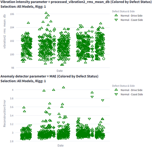
User interface design was critical for practical adoption. An interface inspired by SPC charts visualized AI outputs in familiar formats (Figure 4). Three legend modes support different user needs: “defect legend” for operators, “colored by group legend” for quality engineers investigating root causes, and “colored by sample type legend” for process engineers monitoring system performance.

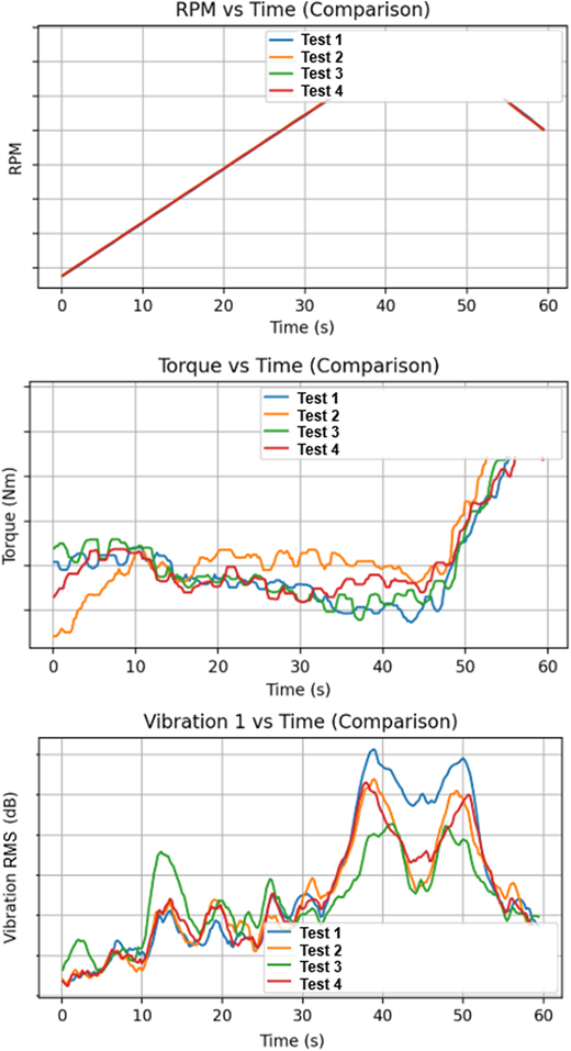
A measurement comparison view enables direct comparison between multiple measurements (Figure 5), helping manufacturing engineers to ensure proper test cycle completion.

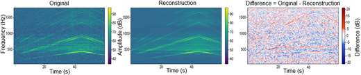
The spectrogram reconstruction view displays the original spectrogram, its reconstruction, and the difference (Figure 6), helping quality engineers understand MAE score by showing where measurements deviate from normal patterns.

The 3D latent space visualization (Figure 7) allows quality engineers to analyze how individual axles relate to others within the AI model's latent space.

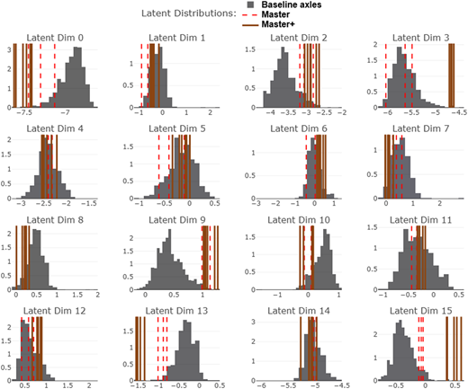
An additional view (Figure 8) shows how each axle's latent dimensions are positioned compared to similar axles, with some dimensions showing significant sensitivity to specific conditions. For example, latent dimensions 3, 13, and 15 were particularly impacted by the increased torque of the Master + axle, providing insights into which “vibration signatures” respond to specific testing conditions.

Together, these complementary views enable different stakeholders to understand AI outputs at multiple levels of detail, from high-level anomaly scores to detailed vibration patterns, supporting both operational decisions and root cause investigation.

This study demonstrates that AI development differs fundamentally from traditional technology implementation (Peretz-Andersson et al., 2024; Bokrantz et al., 2024). Successful AI integration requires building organizational capabilities through coordinated technical and organizational development. Unlike implementing standardized equipment sequentially (specify, purchase, install, adopt), AI development for manufacturing quality control requires to continuously balance technical feasibility and organizational viability. Our empirical evidence demonstrates this through specific interdependencies: model performance depends on data quality, which depends on PLC optimization, which requires maintenance collaboration, which affects production scheduling. These cannot be resolved through upfront planning alone.

The dual PDCA framework operationalizes this insight, providing a coordination mechanism that existing frameworks lack. Technical frameworks (CRISP-DM, MLOps) assume organizational context is given while organizational frameworks (TOE, DOI) assume technical solutions are fixed. Neither addresses coordination itself. The subsequent sections elaborate on these contributions: technical validation (5.1), operational mechanism (5.2), and design principles (5.3).

Despite extensive research demonstrating VAE technical capabilities (Kim and Kim, 2023; Usmani et al., 2024), empirical evidence on VAE performance in real-world manufacturing quality control remains limited (Elía and Pagola, 2025; Jakubowski et al., 2021). This study provides operational validation, demonstrating 12–37% improvement over the traditional RMS method with particular strength (37% improvement) in detecting subtle defects. The VAE model learned the specifics of each test cell and showed robust results across different test cell configurations without requiring equipment standardization. This solved a problem that comes up in real-world deployment situations where different test cells produce different signal characteristics.

Additionally, the study demonstrates that physics-based synthetic defect validation provides an effective technique for building practitioner confidence when ground truth labels are scarce (Xie et al., 2025; Ekwaro-Osire et al., 2025). This enabled direct comparison between AI and traditional methods on known failure modes, providing the technical credibility necessary for organizational acceptance.

While these technical results demonstrate VAE effectiveness, understanding their practical integration requires examining the organizational coordination mechanisms that enabled deployment.

This study identifies a critical need for systemic coordination during AI integration. While recent research (Makarius et al., 2020; Benbya et al., 2021) recognizes that AI requires integrating technical and social elements, our work provides the practical mechanism required to manage that interaction. Our findings suggest that successful integration is not a byproduct of technical excellence alone, but a result of active coordination between departments that are traditionally siloed.

Our dual PDCA cycles framework provides a practical mechanism for this coordination challenge. Unlike existing frameworks that focus on either technical development (CRISP-DM, MLOps) or organizational adoption (TOE, DOI), the dual PDCA cycles allow both to advance in parallel through structured feedback loops (Figure 3). This differs from sequential integration where technical work is performed first, followed by organizational changes. AI creates interdependencies where technical decisions depend on organizational readiness and vice versa. These interdependencies cannot be resolved through upfront planning alone but require continuous coordination during integration.

Traditional STS applications assume joint optimization happens through design decisions made before integration. Our findings reveal something different: AI systems create interdependencies that only become visible during integration itself. The torque regulation challenge illustrates this clearly. Successfully integrating the system required simultaneous changes across five functions. Maintenance adjustments affected model performance, which influenced quality decisions, which required process changes, which affected production flow. This happened not because of poor planning, but because AI inherently creates such interdependencies. We call this “systemic coordination.”

This findings-driven focus identifies how AI creates functional interdependencies between departments that must be managed as a system. It demonstrates that managing this coordination requires parallel process structures (dual PDCA cycles) rather than sequential milestones.

Recent research confirms that successful AI integration requires explicit cross-functional coordination (Bokrantz et al., 2024), resource orchestration (Peretz-Andersson et al., 2024), and human-AI collaboration mechanisms (Krause et al., 2024). Systemic coordination also addresses tensions between traditional quality practices and discovery-driven AI development (Giffen et al., 2025), requiring holistic alignment of people, processes, and technology (Agerskans, 2023).

Our contribution provides STS theory with an operational mechanism, showing how organizations can execute the joint optimization through parallel process structures with explicit feedback loops.

This study reveals specific design principles that enable effective human-AI collaboration in manufacturing quality control contexts.

Graduated severity scores preserve human agency. The MAE scoring method enabled quality engineers to maintain decision-making authority while leveraging AI capabilities for prioritization, contradicting assumptions that effective AI requires minimizing human involvement. Trust calibration, the ability to correctly distinguish when to trust versus distrust an AI system on a case-by-case basis, proves critical for effective collaboration (Zhang et al., 2020). Zhang et al. (2020) demonstrate that confidence scores can help calibrate people's trust in AI predictions, enabling them to appropriately rely on recommendations when certainty is high and exercise independent judgment when certainty is low. Mozannar and Sontag (2020) propose “learning to defer” frameworks where AI systems explicitly recognize limitations and defer to human judgment when confidence is low. Senoner et al. (2024) found that explainable AI with visual heatmaps improved task performance by 7.7% in manufacturing inspection tasks compared to black-box AI.

The latent space visualization enhanced this by enabling practitioners to examine cluster formations and latent space dimension distributions, providing insight into anomaly severity. This multi-layered explainability, combining graduated severity scoring with latent space interpretability, created a nuanced understanding of anomaly context. Krause et al. (2024) emphasize that effective manufacturing systems require integration of human oversight during operation when AI faces uncertainty, precisely the capability our approach provides through graduated MAE scores and visual analytics.

Unlike black-box models requiring post-hoc explainability methods (SHAP, LIME), the VAE model inherently provides both graduated severity scores through MAE reconstruction error and interpretability through its latent space structure. This demonstrates that effective AI collaboration in manufacturing can be achieved by selecting model architectures with built-in transparency that naturally support trust-building, rather than retrofitting explanations on top of black-box models (Kim et al., 2020). The combined mechanisms of MAE score and visual analytics of the latent space address automation bias by requiring human interpretation rather than encouraging automated reliance (Dellermann et al., 2019).

Familiar visualization formats accelerate adoption through cognitive anchoring. Presenting AI outputs in SPC chart formats enabled rapid comprehension by connecting to existing cognitive frameworks. Quality engineers immediately understood complex VAE outputs when presented in familiar formats, demonstrating that interfaces should prioritize cognitive compatibility over technical sophistication (Norman, 2013).

Sadeghi et al. (2024) confirm that workers' acceptance improves when interfaces align with familiar decision-making frameworks. Chong et al. (2022) demonstrate that human confidence in AI evolves as users develop mental models of AI capabilities, with familiar formats accelerating trust development. Bokrantz et al. (2024) provide a comprehensive framework emphasizing that AI interactive attributes, including visualization design, user interface elements, and feedback mechanisms, must align with human cognitive capabilities and existing work practices to ensure successful adoption in manufacturing environments.

These findings provide actionable design principles: (1) provide graduated severity scores rather than binary classifications, (2) combine multiple visualization layers enabling different investigation depths, and (3) anchor new AI outputs in familiar analytical formats to reduce cognitive load and accelerate adoption.

Manufacturing companies integrating AI-based anomaly detection should develop three organizational capabilities:

1. Systemic coordination mechanisms enabling cross-functional problem-solving. Organizations must establish formal coordination structures (workshops, cross-functional teams, regular feedback sessions) that bring together quality, IT, maintenance, and operations during integration, not just during requirements gathering, to enable the transition of AI from a local add-on to a system-level capability.

2. Dual-cycle project structures separating offline technical experimentation from production integration. This enables risk mitigation while maintaining momentum, allowing technical solutions and organizational readiness to develop in parallel before full deployment.

3. Interface designs preserving human agency through graduated severity scoring and familiar visualizations. AI systems should augment rather than replace human expertise, providing tools for prioritization and investigation rather than automated decision-making.

Supported by these capabilities, the phased threshold integration strategy offers a clear roadmap. It begins with severe deviations and gradually tightens the criteria to manage integration in production-critical environments. This approach addresses a fundamental challenge: unlike traditional manufacturing technologies, AI systems cannot be comprehensively validated before deployment (Lebovitz et al., 2021).

For companies with subtle quality issues that conventional methods cannot detect, this approach enables moving from reactive compliance toward proactive quality control (Leberruyer et al., 2023), but success depends on recognizing and managing AI's distinctive systemic coordination requirements.

This study examined capability-building during integration over nine months, capturing the development and initial deployment phase rather than long-term operational sustainability. The qualitative analysis of 20 interviews across seven functions identified core integration themes but represented early-stage rather than mature adoption dynamics. Critical questions about long-term maintenance remain unaddressed: model retraining schedules, performance degradation over time, staffing requirements for ongoing system maintenance, and organizational structures needed to sustain AI systems as production conditions evolve.

The single-case design at one manufacturing plant using one data type limits generalizability. While the systemic coordination construct and dual PDCA mechanism can likely apply across AI integrations, their specific characteristics may vary depending on the context. This study compared VAE performance only against traditional RMS methods, not against alternative AI models. The selection of the VAE model was based on a review of the literature rather than on a systematic empirical comparison in this context. Furthermore, evidence for collaboration-trust linkages remains primarily qualitative; quantitative measures of trust evolution were not used.

Future research should investigate how systemic coordination requirements vary across AI applications and organizational contexts. Comparative studies examining AI integration in different manufacturing sectors could identify which coordination patterns are generalized versus which are context-specific. Longitudinal studies tracking the full integration cycles beyond initial deployment could reveal whether coordination mechanisms remain stable or require adaptation over time (Lebovitz et al., 2021), and whether different governance structures emerge once systems transition from integration to steady-state operations. Controlled comparisons between multiple AI models would establish evidence-based selection criteria for manufacturing anomaly detection applications.

The evolution from anomaly detection to predictive classification represents another important direction. As organizations accumulate operational data, can AI systems progress from identifying deviations to predicting root causes?

Finally, the role of generative AI tools in accelerating integration needs deeper investigation, particularly regarding competency shifts from programming toward socio-technical translation capability (Dellermann et al., 2019).