


This paper examines how the production structure of country-economic complexity impacts gender inequality in Ghana.
Using time-series data spanning from 1995 to 2015, the paper employed the autoregressive distributed lag model as a method of estimation analysis.
The findings reveal a significant negative relationship between economic complexity and gender inequality in the long run, indicating that improvements in economic complexity reduce gender disparities over time. In contrast, the short-term analysis reveals a positive relationship between economic complexity and gender inequality. This suggests that improvements in economic complexity may initially worsen gender inequality, but eventually lead to its reduction.
While previous studies have measure gender inequality using individual indicators such as employment and income differentials, this study adopts a comprehensive measure of gender inequality index which encompasses reproductive health, empowerment (educational attainment and parliamentary representation) and labour market participation. This paper provides findings that are not easily deduced from global or regional panels. More precisely, it helps figure out if a rise in economic complexity leads to a decrease in gender inequality in Ghana given its distinct economic and institutional setting.
1. Introduction
Economic complexity reflects the amount of productive knowledge that a society holds and the combination of capabilities embedded in individuals, organizations and networks that enable the production of a diverse set of sophisticated products (Hidalgo and Hausmann, 2009). Productive capabilities are understood as non-tradable, complementary inputs, including skills, technologies, organizational know-how and institutional arrangements that must be jointly present for production to occur. Unlike individual human capital, which captures education or skills at the worker level, economic complexity captures the collective organization of knowledge at the economy-wide level.
Gender inequality has been a major focus of academic disciplines in various fields (Tovmasyan and Minasyan, 2019). Recently, the issue has gained renewed prominence due to the socioeconomic disruptions caused by the coronavirus pandemic. Some believed these changes really took away the progress previously made towards reducing gender disparities (Kristal and Yaish, 2020). Within the economics discipline, especially labour economics, promoting gender equality has become a significant concern where researchers believe that gender equality will have a positive effect on economic growth and other socio-economic outcomes. This relationship has been extensively examined by numerous scholars and has become a central theme in development and growth economics (Cuberes and Teignier, 2014).
There are empirical evidence showing that female education contributes immensely to economic growth, underlining the key role of women's human capital in enhancing economic performance (Barro, 2001; Dollar and Gatti, 1999; Schultz, 2002). But, Seguino (2000) presents an opposing view by suggesting that gender inequality, which leads to lower female wages, could actually improve a country's export competitiveness and so lead to economic growth. Some studies have been done on the economic impacts of inequality and economic outcomes (for example, Bertay et al., 2020; Schober and Winter-Ebmer, 2011; Seguino, 2000), but the results have not been definitive so far. So, a definitive conclusion is yet to be reached on what is the overall effect of gender inequality on economic development and other economic outcomes (Ndzabela and Lukman, 2023).
Economic complexity and gender inequality are intrinsically linked through the productive capabilities required to sustain increasingly sophisticated economic activities. As economies become more complex, production shifts from simple, low-productivity activities towards more diversified, knowledge-intensive and technologically sophisticated sectors (Hidalgo and Hausmann, 2009; Hidalgo, 2021). Such sectors require a highly skilled and adaptable workforce, thereby increasing the demand for human capital and specialized capabilities irrespective of gender (Hidalgo and Hausmann, 2009; Hausmann et al., 2014). Consequently, economic complexity creates incentives for broader investments in education, skills acquisition and labour force participation, which can contribute to reducing gender disparities in economic opportunities and outcomes. This structural transformation requires a skilled workforce capable of operating in more sophisticated industries.
However, cultural values can influence structural transformation by shaping attitudes towards education, innovation, entrepreneurship, work, gender roles and the adoption of new technologies. Since structural transformation involves the movement of resources from low-productivity sectors (such as traditional agriculture) to higher-productivity sectors (such as manufacturing and modern services), cultural norms can either facilitate or hinder this process. In less complex economies, women are frequently concentrated in low-productivity and vulnerable forms of employment, characterized by lower earnings, informality and limited opportunities for career advancement (Duflo, 2012). Consequently, the demand for educated and skilled labour expands, creating incentives for greater investment in human capital and broader participation in formal labour markets. Nguyen and Su (2021) argue that an increase in formal employment and productive women participation results in better economic complexity and women vulnerability to formal employment reduces economic complexity. These outcomes indicate a woman's labour market participation quality is a key determinant of a country's capacity to build productive capabilities and diversification into elaborate economic activities. Hartmann et al. (2017) argue similarly by demonstrating that complex economies have inclusive economic structures and relatively less inequality. While earlier studies, for example Nguyen and Su (2021), have focused mainly on how gender equality often means increased economic complexity, in contrast, this paper changes the viewpoint completely by examining the extent to which economic complexity has an impact on gender inequality in Ghana. This change of direction is in fact theoretically sound considering that the relationship can be two-way. For instance, while gender equality might lead to economic complexity through more effective utilization of human capital, economic complexity however can help in decreasing gender inequality by creating a higher demand for skilled labour, offering increased formal employment opportunities and developing more inclusive economic structures.
The few existing research on economic complexity and gender inequality focused on cross-country or regional panel data analyses. These kinds of studies generally measure the average effects across countries that have very different productive structures, institutional arrangements and levels of development. So, the estimates obtained might hide significant country-specific correlations and ignore the channels through which economic complexity affects gender outcomes in individual economies.
This paper focuses on Ghana for the following reasons; Ghana has seen major structural changes for the last 30 years (Baah-Boateng and Twum, 2018). One of the most notable changes is the gradual shift from agriculture as the main sector to services, industry and extractive activities like mining and oil production. Many of the changes in production patterns were reflected in the way the country's labour was allocated and Ghana's efforts to diversify its economy. However, there are still gender differences in work, pay and business opportunities despite these economic developments. Social norms, occupational segregation and restricted access to capital are some of the systemic obstacles that prevent women in Ghana from participating in high-value industries (Akotia and Anum, 2015; Baah-Boateng, 2007). It is essential to understand how economic complexity relates to these gendered economic structures to develop policies that support equitable opportunities and inclusive growth.
Again, although Ghana's constitution, in its article 17, states “equality of all citizens before the law, without distinction of origin, race, sex, opinion or religion”, inequality between the sexes still persists in the country. Comparative statistics on gender disparities in Ghana's labour market and business environment reveal that, women account for only 17.85% of paid employees compared to 31.15% of men, while female participation in business ownership stands at 31.6% compared to 68.4% for men (Ghana Statistical Service (GSS) 2024). These statistics demonstrate that women remain underrepresented in formal employment and entrepreneurial activities, which are often the primary channels through which the benefits of structural transformation and economic complexity are transmitted. In the light of this constitutional provision and the existing reality, gender inequality should be understood not only as a violation of human rights but also as a manifestation of social injustice and an economic constraint.
As presented in the World Economic Forum's Global Gender Gap Report (2022) report, Ghana is ranked 108th out of 146 countries, with a gender index score of 0.505. Ghana exhibits significant disparities between women and men compared to other countries on the continent. While Ghana's social dimension has a comparatively high score of 0.984, its economic dimension has a lower score of 0.662. Ghana's score of 0.197 in the empowerment and representation dimension is the most noticeable disparity (African Development Bank, 2023). The overall low gender index of the country is as a result of these discrepancies.
Similarly, Ghana with an Economic Index score of 0.662 means there is a noticeable disparity in economic participation between the sexes. For instance, in Ghana, women ownership to businesses is only 31.6% compared to 68.4% ownership by men (African Development Bank (AfDB), 2023). Furthermore, women only make up 17.85% of paid workers, compared to 31.15% of men (AfDB, 2024). According to the World Economic Forum's Global Gender Gap Report (2024), Ghana's gender parity difference in the economic dimension is 0.338, with a gender index of 0.984, men and women are socially nearly equal.
One of the contributing factors to gender disparity in Ghana is the high rates of educational completion differences between males and females. According to United Nations Educational, Scientific and Cultural Organization (UNESCO) (2023), men complete primary education at a rate of 87.1%, while women complete it at a rate of 89.3%. secondary completion rates are, 63.2% for women and 83.02% for men. Again, according to the Inter-Parliamentary Union (2022), women made up just 26.1% of parliamentarians worldwide. In Ghana, out of the 275 Members of Parliament (MPs) in 2020, only 40 (14.5%) were females, while 85.5% (235 PMs) were males. Similarly, out of the 276 parliamentarians in 2024 elections, only 40 (14.4%) where female while 236 (85.6%) were males. These statistics shows that the proportion of women in Ghana's parliament is still below the global average (26.1%) and the target of 30% female representation in decision-making roles set by the United Nations.
Finally, taking Ghana as a separate case unlike others studies, this paper provides findings that are not easily deduced from global or regional panels. More precisely, it helps figure out if a rise in economic complexity leads to a decrease in gender inequality in Ghana given its distinct economic and institutional setting. Besides, it also helps in identifying if the long-term and short-term relationships are different from those found in general cross-country studies. By doing so, the paper brings some local context-specific considerations to the new research about economic complexity and gender inequality and gives some useful suggestions for the ongoing structural transformation in Ghana.
The remaining section of the study is organized into literature review, method of analysis and conclusion of the study in successive sections.
2. Literature review
This section explains the theoretical and empirical relationships between economic complexity and inequality. This approach ensures that the study is grounded in a robust understanding of existing research. Consequently, the study progresses from theoretical foundations to a review of empirical literature in successive sections.
2.1 Theoretical review
The human capital theory introduced by Becker in 1964 forms that theoretical foundation of this paper. It offers a compelling argument that explain the complex relation between gender inequality and economic complexity. The theory submits that a worker's productivity and earnings are deeply predisposed by investments in skills, training and education. The theory argues that the difference in incomes in society stems from the productivity of labour as a worker is paid based on the marginal product. This standpoint offers a useful basis for evaluating the influence of economic complexity could have on gender inequality. As economies progress on the way to a more sophisticated industries, higher education, labour specialization and innovation becomes crucial, as emphasized by Hidalgo (2021). Whereas Afoakwah et al. (2023), Akotia and Anum (2015) suggest that Ghana's educational inequality has reduced, gender disparity in employment still impede women's participation in the labour market. The Ghana Statistical Service (2025) in attempt to explain the reasons for the persistent gender inequality suggest that women involvement in unpaid domestic work such as child care reduces their ability to earn higher income compare to male counterpart.
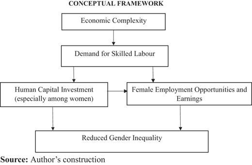
To enhance this theoretical understanding of the paper, the study provides a conceptual framework illustrating the transmission channels through which economic complexity affects gender inequality. The framework highlights that economic complexity promotes the expansion of sophisticated industries, increases demand for skilled labour, encourages investment in human capital and enhances female participation in high-productivity sectors, ultimately contributing to lower gender inequality.
2.2 Empirical review
Empirically, the paper offers strong arguments to support the link between economic complexity and inequality in two main perspectives: First, the paper argues on the relationship between economic complexity and income inequality. Secondly, the link between gender inequality and human capital.
Though, the number of empirical studies that explore the link between economic complexity and inequality is on the rise, most of them focus on income inequality as the primary outcome of distribution. The first major evidence of Hartmann et al. (2017) indicates that countries with more complex production structures tend to have lower levels of income inequality. The authors claim that economic complexity captures a profound change in productive capabilities, as economies diversify into advanced, knowledge-intensive sectors that require skilled labour and are usually linked to more inclusive institutional environments. Similar research on this topic using cross-country data has reinforced that economic complexity is a strong negative determinant of inequality, even when income levels, trade openness and institutional quality are taken into account (Hartmann et al., 2017), which implies that the structural transformation is an important factor affecting income distribution. Taken together, these results are consistent with the idea that reorienting a country's production system can bring a more equitable distribution of income through increased access to higher-productivity jobs.
However, more recent empirical studies suggest that the relationship between economic complexity and inequality is not uniform and may depend on context and level of aggregation. For instance, Nguyen and Su (2021) have demonstrated that the effect of economic complexity on inequality can be nonlinear: the complexity of the economy is related to greater inequality only during the initial phases of development, whereas at the level of highly complex economies it helps to reduce inequality. For this reason, the threshold effects of education, governance and economic openness are only present at higher levels of economic complexity. Additionally, Hartmann and Pinheiro (2024) point out that although economic complexity is correlated with lower inequality at the national level, it is at the same time capable of generating “winner-take-most” scenarios in regions where complex economic activities are concentrated in specific urban locations, leading to a rise in within-country spatial inequality. Such contrasting findings indicate that economic complexity may have distributional effects that depend on the level of institutional capacity and spatial structure; That's why, the complexity–inequality relationship should be considered as very much context-dependent rather than linear everywhere.
Empirical evidence on the relationship between economic complexity and gender inequality is still emerging but increasingly consistent in highlighting important structural linkages. Neagu's study (2021) is the principal and most extensive analysis of different countries' situations, revealing that gains in gender equality measured in employment education health, and political rights greatly lead to a rise in economic complexity, whereas gender gaps in labour market, in particular women being mainly in the vulnerable and informal sector, lessen the level of economic sophistication. This is indicative of a powerful two-way relationship where equality between genders fosters the structural change to production systems which are more complex.
Baah-Boateng and Twum (2018) contribute tremendously to the discussion of the nature, and extent of gender inequality in the Ghanaian labour market, by coming up with evidence revealing that the differences between men and women arising from employment-related issues are not only about the level of employment but also a lot occupational and sectoral segmentation. Their study shows that women in Ghana are mainly in informal, low-quality and vulnerable types of employment, whereas men are more in formal wage employment and higher-quality jobs. This occupational segregation is a reflection of the structural constraints in the labour market such as unequal access to productive resources, entry restriction into higher-paying occupations and the existence of gender-based barriers to job mobility and promotion. Besides, the authors demonstrate quite convincingly that gender inequality in Ghana is largely a matter of the employment structure and not a problem of individual characteristics only; this finding leads to the conclusion that achievement in labour market outcomes will only be possible through changes at the structural level. For economic complexity, these results have a lot of implications as a move towards more advanced and formal sectors might be a solution to this problem of labour market segmentation at least in part by allowing women access to jobs that are not only higher paying but also have better working conditions; This way, women will be more brought-in the concept of narrowing gender gaps in employment quality as well as economic outcomes.
From the forgone empirical discussions, there is paucity of empirical evidence on the link between economic complexity and gender inequality, especially in Ghanaian context. Based on research, the only study that comes close to this argument is Baah-Boateng and Twum (2018) which mainly focus on labour market outcomes. Thus, they explore whether increasing economic complexity leads to the creation of more jobs overall, better employment opportunities, in particular for women and young people. But this paper is concerned with gender disparities. In fact, gender inequality is a concept wider. It includes education, employment and social outcomes rather than employment alone.
3. Methodology
3.1 Data sources and measurement
The study used a time series data spanning from 1995 to 2015 for the analysis. The selection of the study period was determined by data availability. The paper also presents how economic complexity and gender inequality were measured, even though there is a unique measure of economic complexity in the literature. The relevance of economic complexity for labour economics lies in its ability to proxy for the complexity of labour demand. Economies with higher economic complexity tend to generate employment that is more skill-intensive, task-specific and complementary in nature. This has implications for occupational structure, wage inequality, informality and gender disparities in labour market outcomes.
3.2 Measure of economic complexity
Economic complexity index is a measure of the knowledge in a country that translates into the products it makes. To measure the economic complexity of a country is calculated using the revealed comparative advantage (RCA) method, and a discrete matrix is constructed Mcx. This matrix equals 1 if country c exhibits RCA in product x, and 0 otherwise. The matrix Mcx helps measure the range of different products a country exports, while ubiquity describes the number of countries that export a particular product. The economic complexity index (ECI) is computed using the eigenvector derived from the matrix corresponding to the second-largest eigenvalue, normalized by subtracting its mean and dividing by its standard deviation. The ECI typically ranges between −2.8 and +2.8. Higher values indicate a more diversified export structure and a more sophisticated economy, whereas lower values reflect a less complex and less diversified economy.
3.3 Measure of gender inequality
The paper used the gender inequality index (GII) which offers a comprehensive measure of structural gender disparities across various labour market dimensions. It captures gender disparities in three key areas-reproductive health (maternal mortality rate and adolescent birth rate), empowerment (female representation in parliament and educational attainment) and economic participation (labour force participation of men vs women). Given that the productive structure of a country influences sectorial composition and labour requirement, the GII provides a theoretically reliable and policy-relevant measure of gender inequality.
ECI data was sourced from the Atlas of economic complexity (Link to the website). Additionally, the GII, intensive and extensive margins were obtained from the International Monetary Bank (IMF). Labour freedom was obtained from the heritage foundation and trade openness, government expenditure and population were obtained from World Bank's development indicators (see Table 1).
Data sources and measurements
| Variable | Description | Source |
|---|---|---|
| Economic complexity (EC) | Economic complexity index (knowledge stock in production) | ECI |
| Gender inequality (GI) | Gender disparities in three key areas-reproductive health (maternal mortality rate and adolescent birth rate), empowerment (female representation in parliament and educational attainment) and economic participation (labour force participation of men vs women) | IMF |
| Intensive margin (IM) | The increase in work hours or wages of already employed women | IMF |
| Extensive (EM) | The number of new women entering the workforce | IMF |
| Labour Freedom (LF) | Highly flexible labour markets with low government intervention | The Heritage Foundation |
| Trade Openness (TO) | The sum of exports and imports (share of GDP) | WDI |
| Government expenditure (GE) | General government final consumption expenditure (share of GDP) | WDI |
| Population (Pop) | Population density (people per sq. km of land area) | WDI |
3.4 Unit root
The study starts the estimation by testing the stationarity of the data. Employing the augmented Dickey–Fuller test (ADF), the Phillips–Perron (PP) test, Kwiatkowski–Philips–Schmidt–Shin (KPSS) test, the study checked the stationarity of the variables. The unit root test holds that the series exhibit long-term trends or non-zero mean values. The ADF and PP hold the same null hypothesis of non-stationarity and an alternative hypothesis of stationarity. The KPSS holds the reverse hypothesis of ADF and PP. For ADF and PP, the general estimation equation is:
Where = difference of the series at time t, = constant, = slope coefficient, = coefficient of the lagged dependent variable , , …, = coefficient of lagged differences and = error term.
The unit root test assumes that the precision of the α parameter is uniform throughout the passage (i.e. α = β for all i), with the exception that the order of lag α can freely differ. By testing the null hypothesis α = 0 for all i against the alternative hypothesis α < 0 for all I, the unit root test determines whether it is possible to continue integrating the series data. If the null hypothesis is rejected, it indicates that the process of integrating time series data may be continued. In contrast, acceptance of the alternative hypothesis allows for individual series to be integrated. The unit root test is performed on the natural logarithm of a variable at level and on the first difference.
For the KPSS, the unit equation is much simpler, thus expressed below:
Where = the time series, = the deterministic trend and = the error term.
3.5 Estimation strategy
This paper uses the autoregressive distributed lag (ARDL) bounds testing structure first introduced by Pesaran and Shin (1996) and later extended by Pesaran et al. (2001) to explore the long-term relationship between economic complexity and gender inequality. The ARDL bounds testing method has an edge over the traditional cointegration methods like the residual-based method of Engle and Granger (1987) as well as the full maximum likelihood procedures introduced by Johansen (1988, 1991) and Johansen and Juselius (1994). One major benefit of ARDL method is that it does not necessitate all variables being integrated of the same order. Versus standard cointegration methods, ARDL is applicable when variables are integrated of order zero [I(0)], order one [I(1)] or even a mixture of both, as long as none of the variables is integrated of order two [I(2)]. This feature of ARDL model makes it a great choice for empirical work where variables have mixed orders of integration.
Furthermore, the ARDL approach offers several other benefits, the traditional cointegration techniques generally rely on estimating a long-run relation in a system of equations, while ARDL uses only one single reduced form equation. This makes the estimation process much easier (Pesaran and Shin, 1996). Also, the ARDL method is robust enough to generate long-run results and dependable t-statistics even when there are endogenous regressors (Odhiambo, 2010). Besides this, one of the major advantages of the ARDL approach is that it can work well with small sample sizes, whereas most traditional cointegration techniques, including the Johansen and Juselius (1994) method, tend to be very sensitive to the sample size. Because of these merits, the ARDL bounds testing method is mostly considered a reliable and adaptable way of investigating long-run relations among variables and has become very popular in empirical studies. Based on the literature review and data constraints, the paper sets out this double-log specification as follows:
The error term is denoted by , and the difference operator is represented by Δ. Changes in the short and long terms are denoted by the parameters ; i = 1, …,4 and ∂i; i = 1, …,4, respectively.
Equation (5)is subjected to the following error correction model (ECM) in the study to account for both short- and long-term estimates. The model is essentially an augmented production function estimated in a dynamic ARDL framework, where economic complexity serves as the key independent variable.
To estimate Equation (3), the literature raises endogeneity concern between gender inequality and economic growth. A key concern is reverse causality, economic development may reduce gender inequality, while greater gender equality can also promote development (Duflo, 2012; Stotsky, 2006; International Monetary Fund. Research Dept, 2013). One potential way to address these issues is through instrumental variable techniques, though identifying a valid instrument that affects growth solely through gender inequality remains a complex challenge. Bertay et al. (2025) suggest that an effective way to resolve this endogeneity problem is to instrument economic growth using the extensive and intensive margins of employment. On the extensive margin, improved gender equality expands the labour pool by increasing female labour force participation, leading to productivity gains from a more diverse and skilled workforce (Cuberes and Teignier, 2016; Kazandjian et al., 2019). On the intensive margin, it allows women to fully develop their career potential for example, through greater opportunities for advancement which also contributes to economic growth (Islam and Amin, 2016). Therefore, the paper instruments economic growth with both the intensive and extensive margins. As follows:
Where: the notation of (GI), (EC), (TO), (LF), (PoP), (GE), (IM) and (EM) denotes gender inequality, economic complexity, trade openness, labour freedom, government expenditure, population, intensive and extensive margins. The coefficient of the error correction term captures the existence of long-run causality, while the joint F-test on the coefficients of the first-differenced explanatory variables provides evidence of short-run causality. The symbol represents the first-difference operator. The term denotes the stationary error term in Equation (4). The parameter refers to the optimal lag length of the ARDL model, which corresponds to lags in the ECM. In an ARDL model, short-run causality is typically examined using a Wald test (F-test or Chi-square test) on the joint significance of the lagged differenced explanatory variables. Long-run causality is inferred from the significance of the error correction term (ECT).
Table 2 presents the descriptive statistics of the variables used in the analysis. The results show that Gender inequality (GI) variable has a mean value of 0.585, a standard deviation of 0.023 and ranges from 0.553 to 0.629. This indicates that, on average, the Ghana experienced a moderate to high level of gender inequality during the observed period. Suggesting there is significant disparities between men and women in terms of reproductive health and labour market participation. The standard deviation of 0.023 suggests that gender inequality remained fairly stable, with no major policy shifts or shocks that drastically changed the status of gender equality in the short term.
Descriptive statistics
| Variable | Obs | Mean | SD | Max | Min |
|---|---|---|---|---|---|
| GI | 21 | 0.585 | 0.023 | 0.629 | 0.553 |
| EC | 21 | −0.949 | 0.204 | −0.532 | −1.371 |
| PoP | 21 | 22.650 | 3.556 | 28.696 | 17.399 |
| LF | 21 | 54.409 | 5.252 | 62.9 | 45.3 |
| GE | 21 | 10.347 | 2.179 | 15.308 | 7.0694 |
| TO | 21 | 82.047 | 16.660 | 116.048 | 57.423 |
| IM | 21 | 4.107 | 0.199 | 4.589 | 3.704 |
| EM | 21 | 0.570 | 0.192 | 0.938 | 0.150 |
Again, the data reveal that over the study period, the economic complexity (EC) had a mean value of −0.949, indicating that the country's economy was relatively less complex. A negative EC suggests limited diversity and low sophistication in the country's export basket, often dominated by raw materials or low-technology goods (Hidalgo and Hausmann, 2009). The standard deviation of 0.204 shows moderate variability in economic complexity over time, implying that while some structural changes may have occurred, they were not substantial. The index ranged from −1.371 to −0.532, meaning that even at its most diversified point, the economy remained below the global complexity average. This persistent low complexity may reflect a continued reliance on a narrow range of exports, limited industrial transformation and underdevelopment of knowledge-intensive sectors.
4. Results and discussion
This section presents and analyses the empirical findings on the extent to which economic complexity impact of gender inequality in Ghana over the period 1995–2015. The discussion begins with an examination of the time-series characteristics of the variables and the results of the ARDL bounds test for cointegration. This is followed by the presentation of the long-run and short-run estimates, together with the relevant diagnostic and stability tests used to assess the robustness and reliability of the estimated model.
4.1 Unit root and cointegration test results
Since the validity of the ARDL approach rests on the consideration of the variables as integrated of order zero [I(0)], order one [I(1)] or a mixture of the two, it is absolutely imperative to check their stationarity features first. This initial step will prevent any one of the variables from being unknown integrated of order two [I(2)] or more, which would prohibit the use of the ARDL technique. As single unit root tests suffer from significant shortcomings, the present investigation uses a few unit root testing methods like the Phillips–Perron (PP) test crafted by Phillips and Perron (1988). The null hypothesis of unit root could not be rejected in some cases. This suggests some variables are not stationary at levels. Since the divergence of the variable from its mean affect the long-run equilibrium condition, the series was purged of this trend through first differencing. The study further checked whether there is a long-run relationship between the variables. The result revealed that the variables are integrated on of other I(0) and I(1) as shown in Table 3 as follows.
Augmented Dickey–Fuller test for unit root
| Series | Order | ADF% | Test statistics |
|---|---|---|---|
| EC | Level | −3.000 | −2.464 |
| 1st Difference | −8.124*** | ||
| GI | Level | −3.000 | −0.679 |
| 1st Difference | −4.400*** | ||
| PoP | Level | −3.000 | −0.828 |
| 1st Difference | −4.489*** | ||
| LF | Level | −3.000 | −2.032 |
| 1st Difference | −4.466*** | ||
| GE | Level | −3.000 | −0.971 |
| 1st Difference | −4.936*** | ||
| IM | Level | −3.000 | −3.630** |
| 1st Difference | −1.515 | ||
| EM | Level | −3.000 | −1.260 |
| 1st Difference | −4.382*** | ||
| TO | Level | −3.000 | −3.122** |
| 1st Difference | −2.209 |
Note(s): *** and ** denoted a rejection of the null hypothesis of unit root at 1% and 5% respectively
4.2 The ARDL bound co-integration test
Using the bounds test co-integration technique (Pesaran et al., 2001), the study established that the F-statistics (24.646) is greater than the critical values of the upper bound (3.50). Therefore, the null hypothesis of no co-integration was rejected in favour of the alternative hypothesis, meaning there is a long-run relationship between the dependent and independent variables. The small sample size in this study makes the ARDL model more suitable for the analysis. Again, the ARDL co-integration model produces unbiased long-run estimates, which makes it more preferred.
From Table 3, the study conclude that all the variables used in the study cointegrated. That is, there is a long-run relationship between the entire variable in this study. Hence, the choice for the co-integrating-ARDL model (ARDL-ECM). This model presents both short-run and long-run results and minimizes biased results. Table 5 presents the co-integration equations. The Star (*) denoted the best lag order per the information criterion.
4.3 Lag length selection criteria
The study used an econometric approach for the optimum lag selection. From Table 4, the most dominant lag length was lag 2, as FPE, AIC and HQ suggested. Therefore, the study used a maximum lag of two. Based on the maximum lag selection criteria, the study specified the estimable model as ARDL (1 2 2 2 2 2).
The bounds test for co-integration
| Dependent variable | F-statistics | Co-integration | Model to estimate |
|---|---|---|---|
| EC | FEC 10.228 tEC = −3.062 | Yes | ECM |
| PoP | FPop = 9.117 tPoP = −4.269 | Yes | ECM |
| LF | FLF = 9.916 tLF = 5.73 | Yes | ECM |
| GE | FGE = 11.105 tGE = −4.323 | Yes | ECM |
| TO | FTO = 9.120 tTO = −3.621 | Yes | ECM |
| IM | FIM = 15.950 tIM = −5.579 | Yes | ECM |
| EM | FEM = 13.571 tEM = −5.209 | Yes | ECM |
| ARDL (1 0 1 1 0 1 1 0) K = 7 | F-statistics (24.646) | Upper bound I(1) (3.50) |
Note(s): EC = Economic complexity, PoP = population, LF = labour freedom, GE = government expenditure, TO = trade, IM = intensive margin, EM = extensive margin
AIC denotes Akaike information criterion; LR denotes Sequential modified test statistic, FPE denotes Final prediction error, HQ denotes Hannan Quinn information criterion, SC denotes Schwarz information criterion. The study choses the AIC because it gives the lowest value as shown in Table 5.
Co-integration: lag length criteria
| Lag | Ll | LR | P | FPE | AIC | HQ | SC |
|---|---|---|---|---|---|---|---|
| 0 | −3.26959 | 0.168395 | 1.02995 | 1.07088 | 1.32674* | ||
| 1 | −2.37889 | 1.7814 | 0.182 | 0.173327 | 1.0421 | 1.08984 | 1.38836 |
| 2 | −0.727721 | 3.3023 | 0.069 | 0.16505* | 0.969747* | 1.02431* | 1.36547 |
| 3 | 0.130734 | 1.7169 | 0.190 | 0.173116 | 0.985474 | 1.04686 | 1.43066 |
| 4 | 0.132311 | 0.00315 | 0.955 | 0.201934 | 1.09641 | 1.16462 | 1.59106 |
4.4 Estimated results of the ARDL model
The long-run estimates reveal a negative and statistically significant relationship between economic complexity and gender inequality. The coefficient of −0.145 means that a one-unit increase in economic complexity leads to a 0.145-unit reduction in gender inequality, all else being equal. In practical terms, the coefficient means that if everything else remains equal, a one-point rise in the ECI results in a decrease of 0.145 points in the GII. Given that the GII is an index where higher levels indicate more inequality and lower levels indicate more equality, the negative coefficient suggests that the higher productive sophistication of Ghana is linked to the improvements in women's conditions compared to men. The coefficient of −0.145 generally shows that, besides being a driver of economic growth, economic complexity also is key in reducing gender inequality in Ghana. It indicates that as Ghana moves into a more advanced and varied economy, it will likely open up a whole range of opportunities for women, empower them more and help close the gender gap.
The economic significance of the finding largely depends on what economic complexity stands for. In simple terms, economic complexity refers to how much an economy is equipped with the kind of productive knowledge, technological capabilities and institutional capacity that are necessary to manufacture advanced goods and services. At the same time as Ghana is gradually shifting from dependence on primary commodities like cocoa, gold and crude oil to the development of diversified manufacturing and knowledge-intensive sectors, the demand for equipped workforce grows. Such a transformation opens up chances for females to get education, build skills, engage in formal employment and move into better-paying positions. Because of this, economic complexity might ease the traditional constraints that limit women to time-consuming and low-result activities and increase their economic participation and role in decision-making.
This is clearly good news for women in Ghana. If structural transformation is to be seen only as another tool for achieving economic growth, it will be a great disservice to the women. A more diversified and sophisticated economy is going to lead to creation of more jobs in sectors like finance IT telecom, professional services, highly-technical manufacturing and other skill-intensive industries where the main drivers of success will be educational level and professional competence rather than conforming to traditional gender roles. Women's increased presence and involvement in these sectors will not only raise their earnings but also lessen their concentration in certain types of jobs, lead to their economic empowerment and give them the capacity to allocate resources not only for their own and their families health and education but also for other areas.
The result also extends to areas outside the labour market. Since the GII accounts for aspects like reproductive health, empowerment and labour market participation, a decline in gender inequality indicates a general upturn in women's welfare. With the rise of economic complexity, women could see more presence in top managerial posts, heightened political engagement, enhanced schooling results and greater access to economic resources. Because of this, the coefficient the paper has estimated indicates that policy measures focused on enlarging Ghana's productive capacities and export sophistication can, at the same time, drive the country's gender equality goals.
In contrast, the short-run coefficient shows a positive relationship economic complexity and gender inequality. For every unit increase in economic complexity, gender inequality increases by 0.077 units. This short-run effect is statistically significant at 5% level. It means that initial increases in economic complexity might actually lead to a short-term rise in gender inequality before the longer-term benefits materialize. The positive short-run coefficient reported in this paper could be attributed to transitional adjustment effect due to the reallocation of economic opportunities during the initial period of structural upgrading rather than as a proof that economic complexity will always lead to more gender inequality.
In particular, improvement in economic complexity is generally linked with an initial period of structural adjustment when the benefits of productive upgrading are not immediately and evenly spread among people. At the beginning of structural transformation, highly-developed sectors emerging mainly require specialized skills, technical knowledge and educational qualifications which may not be available to everyone. Considering that there are still differences between men and women in access to productive resources, formal jobs, training for skills and leadership positions in Ghana, women could encounter more difficulties at first in gaining access to the opportunities that come from the growth of the complex economic activities. That means, gender imbalances may be exacerbated temporarily as the economy moves to a more advanced productive structure before the gender benefits of the structural transformation become visible.
Accounting for the control variables, the findings show population density is one of the factors influencing gender inequality since it increases gender inequality but eventually reduces it soon. The positive short-term effect could be an indication of the initial challenges brought about by rapid population growth such as increased competition for scarce jobs, limited educational resources and public services that unconsciously end up affecting women more thereby, widening gender inequalities. Even so soon a higher population density can mean the spread of cities, the benefits of being close to one another, better familiarity with education, healthcare and other facilities as well as the labour market resulting in a decrease in gender inequality. The same way, labour freedom, trade openness, intensive margins and government expenditure do lessen gender inequality even in the short term. Based on this evidence, more flexibility in the labour market, a higher level of integration with international markets, the deepening of current export activities and government spending can open up fresh opportunities for women's employment and economic participation immediately. However, the significant and large coefficients of labour freedom, trade openness, and government expenditure soon indicate that the advantages of these variables are not equally shared automatically over time. In fact, without gender-sensitive policies, the liberalization of the labour market, the increase in trade and government spending could mainly benefit men, who are typically better positioned in the formal, high-paying and export-oriented sectors, this way leading to an increase in gender inequality over time. Besides, although the coefficient linked to intensive margins turns positive eventually, it still loses statistical significance, which implies that the growth of existing export activities is not a main driver of gender inequality in Ghana over time.
The differences between short-run and long-run coefficients found here are, from a theoretical point of view, one of the features of the dynamic adjustment process captured by the model. Over time, the variables like intensive Margin (IM), government expenditure (GE) and trade openness (TO) may have direct and sometimes distortionary effects on gender inequality most of the time due to factors like adjustment costs, sectoral reallocation and institutional rigidities. Such short-term impacts can be understood as hiatuses of labour market frictions, changes in consumption habits and public spending allocation that take place before the economy adjusts fully to changes in external and fiscal conditions.
However, the long-term coefficients indicate the final equilibrium-state relationships, after all the adjustments have been done. Here, the lack of significance or the flip of sign of IM over time (0.107) may be understood as the initial short-run effects fading away over time, pointing out that imports no longer maintain a separate and continuous influence on gender inequality after structural adjustments are made. This reasoning can be extended to GE and TO, where short-run effects could be interpreted as the immediate redistributive or sectoral dynamics, whereas long-run effects signify the stable institutional and structural states.
Also, the coefficient of the ECM is negative and significant in the model (−0.74). This value signifies that the economic complexity and gender inequality adjust to their equilibrium with a speed of 74%. This coefficient means that short-run deviations from the long-run equilibrium between economic complexity and gender inequality are corrected within one year. The change is fairly quick, which implies that even when the system is temporarily thrown out of balance or experiences a shock, it almost immediately goes back to its long-run equilibrium state.
In practical point of view, this finding means that variables like economic complexity or gender inequality can only be affected for the short term at most by a policy change, economic shocks from external source or a change in the structure of production in Ghana, for instance. In fact, the dynamics of the variables revert quite strongly to their long-run equilibrium path over a short period of time.
This finding is linked to a larger set of empirical papers on ARDL and ECMs in development economics, in which adjustment speeds are roughly 29%–99% per period, see (Menegaki, 2019) for examples. Factors like the country context, types of variables and model specification are known to determine the speed. So, the estimated coefficient of around 0.74 implies that adjustment occurs quite fast, which is in fact signalling strong harmonization over time between the variables in the Ghanaian economy.
4.4.1 Diagnostics test
The middle part of Table 6 presents the outcomes of the diagnostic tests for serial correlation, heteroskedasticity and normality. The findings indicate that the model does not suffer from issues related to serial correlation or heteroskedasticity. Additionally, the Jarque–Bera test confirms that the variables follow a normal distribution.
ARDL assessment results
| Test statistic | Value | Signif | 5% |
|---|---|---|---|
| F-bounds test | |||
| F-statistic | 24.646 | I(0) | 2.32 |
| I(1) | 3.50 | ||
| t-bounds test | |||
| t-statistic | −2.489 | I(0) | −2.86 |
| I(1) | −4.57 | ||
| Variable | Coefficient | SE | t-statistic |
|---|---|---|---|
| Long-run level relationship | |||
| EC | −0.1452** | 0 0.0506 | −2.87 |
| PoP | −0.1409*** | 0.0345 | −4.08 |
| LF | 0.0025** | 0.0011 | 2.11 |
| GE | 0.0087*** | 0.0028 | 3.10 |
| TO | 0.0027*** | 0.0006 | 4.42 |
| IM | 0.1067 | 0.0573 | 1.86 |
| EM | −0.3571*** | 0.0559 | −6.39 |
| Test | Value | p-value | Decision |
|---|---|---|---|
| Diagnostic tests outcomes | |||
| Heteroscedasticity | 1.041 | 0.4093 | Homoscedastic |
| Serial correlation | 2.0302 | 0.695 | No serial correlation |
| CUSUM | Not stable | ||
| CUSUM SQUARE | Stable | ||
| Variable | Coefficient | S.E. | t-statistic |
|---|---|---|---|
| Short-run ECM results | |||
| Cointeq(−1) | −0.7375*** | 0.0735 | −10.03 |
| EC | 0.0776** | 0.0270 | 2.88 |
| PoP | 0.0619*** | 0.0195 | 3.17 |
| LF | −0.0021** | 0.0009 | −2.38 |
| IM | −0.3632*** | 0.0582 | −6.23 |
| TO | −0.0138 | 0.0260 | −0.53 |
| GE | −0.0121 | 0.0296 | −0.41 |
Note(s): *** and ** denotes 1%, and 5% levels of significance respectively
The normality and stability tests show that the model is normal and stable. This suggests that the results discussed are not spurious, as evidenced in the Cusum-Square graph. While the CUSUM shows a deviation of the model from its long run, the Cusum-Square shows that any deviation from the equilibrium path will be corrected towards long-run equilibrium. The results indicate that the model coefficients remain structurally stable over time.
The CUSUMSQ test as presented (Figure 1) explains whether or not the estimated coefficients changed over time during the 20-year analysis period. The CUSUMSQ statistic does not get beyond the 5% critical bounds, showing that variance of the regression errors as well as the estimated model parameters are not subjected to substantial structural changes. Combining evidence from the test, the model estimated is structurally stable for the 20 years with no indication of major regime changes, parameter instabilities or structural breaks that would be detrimental to the reliability of the estimated relationships. This stability is even more crucial since the study period is marked by many major economic, institutional and policy adjustments; and the results show that these changes did not essentially change the estimated relationships among the variables. That means, the coefficient estimates can be regarded as capturing the relatively persistent patterns over the study period rather than the patterns specific to a particular sub-period.
 The line graph presents the Cusum-Square test over a period from 1995 to 2015. The x-axis represents the years, ranging from 1995 to 2015, while the y-axis represents the Cusum-Square values, ranging from negative 0.5 to 1.5. The graph includes four lines: a blue line representing the Cusum-Square values, a green line representing the upper critical bound, an orange line representing the mean, and a red line representing the lower critical bound. The blue line starts below zero around 2000, rises above zero around 2005, and continues to increase with some fluctuations, reaching above 1 by 2015. The green line shows a steady upward trend, the orange line shows a moderate upward trend, and the red line shows a steady upward trend but at a slower rate compared to the green line. All values are approximated.
Cusum-Square test. Source: Author's own work
The line graph presents the Cusum-Square test over a period from 1995 to 2015. The x-axis represents the years, ranging from 1995 to 2015, while the y-axis represents the Cusum-Square values, ranging from negative 0.5 to 1.5. The graph includes four lines: a blue line representing the Cusum-Square values, a green line representing the upper critical bound, an orange line representing the mean, and a red line representing the lower critical bound. The blue line starts below zero around 2000, rises above zero around 2005, and continues to increase with some fluctuations, reaching above 1 by 2015. The green line shows a steady upward trend, the orange line shows a moderate upward trend, and the red line shows a steady upward trend but at a slower rate compared to the green line. All values are approximated.Cusum-Square test. Source: Author's own work
5. Conclusion and policy recommendations
This paper explains the how economic complexity affects gender inequality in Ghana. Gender inequality was measured using GII and the ECI is used as a measured of economic complexity. Utilizing annual data from 1995 to 2015 and applying the ARDL approach appropriate due to the mixed stationarity of variables, the paper evaluates the characteristics of the data by examining the long-run relationship between economic complexity and gender inequality. The ARDL bounds test confirmed a long-term association among the variables. The result reveals a negative effect of economic complexity on gender inequality, suggesting that improvements in the productive structure of Ghana can contribute meaningfully to reducing gender inequality in the long-run, contrary to the short-run positive effect. The positive short-run coefficient reported in this paper could be attributed to transitional adjustment effect due to the reallocation of economic opportunities during the initial period of structural upgrading rather than as a proof that economic complexity will always lead to more gender inequality. The study therefore concludes that economic complexity has the potential to bridge these gaps by fostering inclusive economic systems that support women's involvement in high-productivity sectors, but targeted interventions may be needed in the short term to ensure that women can access and benefit from opportunities created by complex economic activities. Based on these findings, the study recommends that policymakers design and implement policies that improve the level of economic complexity, thereby accelerating the long-run gender equality gains associated with economic complexity in Ghana.

