


Increased fiscal autonomy is often identified in studies as leading to improved financial health in local governments, while research finds those depending heavily on funding from other levels of government suffer a decline in financial health.
We analyze financial information from municipalities in nine different countries to gain a more nuanced understanding of this relationship.
Our analysis reveals a more complex picture, in which greater fiscal autonomy may benefit long-term solvency but challenge short-term liquidity and budget stability, potentially impacting overall financial health.
Our research reveals that there is no linear relationships between financial autonomy and financial health.
Introduction
Studies show that local government (LG) systems around the world vary in the way they approach public governance (Kuhlmann and Wollmann, 2019) and financing of their activities (Maher and Deller, 2011). These studies show that these varying approaches significantly impact LG financial performance (Geissler et al., 2019; Geissler and Wegrich, 2021). Broadly, the existing literature suggests that LGs with greater fiscal autonomy are more financially healthy, while greater dependency on other levels of government for funding is associated with increased financial distress (Hendrick, 2011; McDonald and Maher, 2020).
However, most of these studies focus on a single country (Citro et al., 2018; De Matteis and Preite, 2018; Hruza, 2015; Padovani et al., 2018) and take a narrow approach to measuring financial health. Many studies overlook that financial health is multifaceted, with various factors interacting, suggesting a nuanced complexity to the relationship between fiscal autonomy and financial well-being (Clark, 2015). This study aims to fill these two abovementioned gaps by taking a multi-country perspective to explore the ways in which fiscal autonomy impacts various dimensions of financial health. Using comparable financial information from municipalities in six European countries (Bosnia and Herzegovina, the Czech Republic, France, Italy, Portugal, and Spain) and two US states (Colorado and Virginia), the analysis tests the relationship between fiscal autonomy and financial health across countries incorporating a range of factors. These countries are chosen because they represent diverse LG systems (Kuhlmann and Wollmann, 2019), they enjoy local autonomy (Ladner et al., 2023), and comparable financial data is available (Padovani et al., 2018).
This research contributes to the debate on the financial viability of LGs, emphasizing the role of fiscal autonomy. Fiscal autonomy, defined as the ability to set self-rules for managing one’s own financial affairs, is rooted in the conviction that devolution and decentralization can shift the focus from bureaucratic procedures to managerial initiatives (Pollitt, 1993; Dunleavy and Hood, 1994; Ferlie et al., 1996). This shift is a cornerstone of the New Public Management (NPM) paradigm (Hood, 1991, 1995). Ideas developed under NPM theory highlight that fiscal autonomy is essential to substantiate the demand for responsibility by LGs (Mussari, 1996). Thus, fiscal autonomy becomes a critical element of NPM, facilitating the implementation of managerial principles and enhancing the efficacy and accountability of local governance. This NPM idea is grounded in antecedent theories of fiscal federalism, decentralization theory, and agency theory. Fiscal federalism examines how decentralizing fiscal responsibilities can lead to more efficient and responsive governance (Oates, 1972). Decentralization theory argues that delegating fiscal responsibilities results in improved governance outcomes by making governments more accountable and responsive to local needs (Tiebout, 1956). Agency theory explores the relationship between principals (citizens) and agents (government officials), focusing on how fiscal autonomy can align the interests of government officials with those of citizens (Laffont and Martimort, 2002). These foundational theories collectively underpin the NPM emphasis on fiscal autonomy as a means to enhance local governance.
Despite the substantial body of literature on the topic, there remains a gap in comparative studies that ascertain whether the positive impact of fiscal autonomy on the management of public resources holds true across countries. Our analysis centers on periods of economic stability, drawing on the pertinent literature within this context. For insights into financial instability, shocks, and crises, reference should be made to works such as Martell and Moldogaziev (2023). This study undertakes a cross-country analysis and moves beyond a focus on administrative and accounting traditions to understand how the nuances of the relationship between fiscal autonomy and financial health emerge at an international level (Jones and Walker, 2007; Gomez et al., 2024). It introduces an innovative method to compare LGs across countries by reclassifying financial information from different accounting systems, addressing the absence of widely accepted and uniform international standards. Thus, it also contributes at a practical level, offering a tool to assess fiscal conditions at the local level, complementing ratings from international agencies that mainly cover national and regional governments (Johnson and Kriz, 2005; Peppe and Unal, 2022).
Literature review
Financial health in LGs encompasses both positive stability and sustainability, contrasting with financial distress, which signifies a struggle to meet financial obligations (Gardini and Grossi, 2018). Termed alternatively as fiscal health, financial position, fiscal stress, or fiscal crisis (Cabaleiro et al., 2013), its definitions vary from the inability to meet obligations to broader criteria including taxation levels, service provision capabilities, and short- and long-term financial perspectives (Lin and Raman, 1998; Carmeli and Cohen, 2001; Kloha et al., 2005; Wang et al., 2007; Jones and Walker, 2007; Zafra-Gomez et al., 2009). In our study, financial health is defined as the municipality’s ability to balance its budget and meet current and future obligations. The concept of financial health in LGs remains complex and multifaceted, encompassing a dynamic interaction of various dimensions (Cabaleiro et al., 2013). While literature often focuses on specific aspects such as debt repayment (Jones and Walker, 2007; Maher and Deller, 2011; Bastida et al., 2014; McDonald and Maher, 2020; Martell, 2008) or annual budget commitments (Carmeli and Cohen, 2001; Chapman, 1988; Kloha et al., 2005), comprehensive measurement across multiple dimensions is less common (Clark, 2015). Widely recognized dimensions of LGs’ financial health (Groves et al., 2003; Hendrick, 2011; Jacob and Hendrick, 2012) include cash solvency – assessing liquidity and effective cash management to meet immediate liabilities crucial for avoiding payment delays and service disruptions, budget solvency – evaluating whether annual revenues cover expenditures without resorting to borrowing or reserves, long-run solvency – the impact of long-term obligations both in terms of impact on current budget (debt capacity) or future level of taxation or services (affordability) (Kriz and Wang, 2013), and service-level solvency – the LG capacity to deliver necessary public services influencing service quality and quantity.
The above review depicts a scenario where there is no agreement about the measures of financial health across countries (Gomez et al., 2024). Moreover, despite Pollitt’s (2008) seminal work highlighting the critical role of time-related factors, subsequent studies have largely overlooked these aspects when examining the effects of fiscal autonomy on the financial viability of LGs and focused mainly on one of these dimensions. Even studies that have adopted a multifaceted perspective on financial health—such as Martell and Moldogaziev (2023), which examined LG ability to meet current expenditures, capital expenditures, and debt obligations—did not focus on intertemporal relationships in their analyses. This gap represents a substantial issue in the literature about fiscal federalism, decentralization, and agency theories. Our study aims to address this gap by integrating a temporal perspective into the analysis of fiscal autonomy and its implications for LG financial health. Hence, we follow the extant literature and adopted three broad indicators of financial health available across countries (Kloha et al., 2005; Gardini and Grossi, 2018) to appreciate the trends of financial behavior. Specifically, we consider cash solvency, which looks at the very short-term ability to pay liabilities; budget solvency, which relates to the capacity to balance revenues and expenditures within an annual period; and long-run solvency, which focuses on the impact of debt on the current budget and the government’s debt capacity. We focused on dimensions of financial health that are purely financial, as service-level solvency information is neither available nor comparable across countries due to the challenges in assessing and standardizing service-level performance internationally (Padovani and Scorsone, 2009).
Measuring financial health in local governments across countries
A consistent body of literature focuses on the metrics and determinants of LG financial health depending on the definitions used, ranging from a set of purely financial indicators (Wang et al., 2007; Rivenbark et al., 2010) to indicators of financial conditions, social and economic characteristics, and quality of services provided. These include both external and internal factors (Zafra-Gomez et al., 2009). The literature suggests that various indicators have been used, each tailored to the specific context and purpose of measuring financial health (Justice and Scorsone, 2012). Regardless of how indicators are defined, studies identify revenue-generating capacity or fiscal autonomy as one of the strongest impacts on LG financial health (e.g. Jones and Walker, 2007). This measure has been used either as a component of LG financial health or as a determinant (Bisogno et al., 2017). Furthermore, the practice of deconstructing financial health into its components and examining how certain components relate to others has already been widely implemented (e.g. Bisogno et al., 2019).
Adding the cross-country dimension
In the public sector, including at the LG level, financial information is presented in different ways in different countries. Research contrasts government financial reporting with government statistics, which have different aims and scopes (e.g. Jorge et al., 2014; Dasì et al., 2016). Also discussed is the dichotomy between cash-based and accrual accounting systems and their effective use (e.g. Lapsley et al., 2009; Caruana et al., 2019). While accrual accounting has been more widely adopted, traditional accounting systems coexist and may be more useful in certain situations (Padovani et al., 2018; Padovani and Iacuzzi, 2021).
Moreover, a vast literature explores various techniques and approaches beyond accounting for measuring LG financial health (Padovani and Scorsone, 2011). Recent research has reclassified financial data from official reports, combining hybrid approaches and accounting systems, to compare LG financial health in large cities (Padovani et al., 2018; Heichlinger et al., 2021a), but not for all LGs.
From a practitioner perspective, credit agencies compare the financial health of public entities to establish creditworthiness. Credit ratings synthesize LG financial health by assessing financial, debt, economic, and administrative conditions (Johnson and Kriz, 2005; Levy and Pauzner, 2014) from a qualitative perspective (Park, 2004; Landry and McCarty, 2007). As these assessments are expensive undertakings, they are mostly available for national and regional governments and only a few large LGs (Peppe and Unal, 2022).
Factors determining financial health
While this paper focuses on fiscal autonomy, the literature identifies numerous determinants of LG financial health, which can be broadly categorized into two groups: (1) external determinants, such as national institutions, service demand and economic wealth, and (2) internal, such as fiscal autonomy. Therefore, our objective is to explore these dimensions to assess the relative importance of fiscal autonomy within the broader framework of financial health.
National institutions
Several external factors ‒ those outside the local environment and thus outside the LG management domain ‒ affect LGs’ financial health. First, LG financial health can be influenced by national context, in terms of each country’s institutional framework, fiscal rules, and administrative and cultural traditions. New institutional theory suggests that cultural beliefs and rules influence decision making (Lounsbury, 2008). Institutional factors and fiscal rules, including bankruptcy and bailouts procedures, legal debt burden limits, accounting systems, and auditing/supervision procedures, can impact financial health at the local level (Canuto and Liu, 2013; Padovani and Scorsone, 2011). Central governments have developed various insolvency procedures with different levels of effectiveness (Person, 2021). Legal debt burden limits and other fiscal rules are also commonly determined at the central level (Allers and de Natris, 2021; Sutherland et al., 2018).
The accounting system adopted determines the perception of LG financial health and the adoption of global accounting standards like accrual and the International Public Sector Accounting Standards (IPSAS) has led to similar outcomes across national boundaries (Polzer et al., 2021), yet there are no international universal standards; even in the European Union there are different levels of maturity for accrual standards (European Commission, 2020). Auditing and supervision activities also vary significantly across countries (Geissler and Wegrich, 2021). Different administrative traditions and structures may indeed influence LGs’ financial health. Kuhlmann and Wollmann (2019) identify three profiles with structural models of administration: a functional profile, a territorial profile, and a political profile. Other authors identify vertical coordination patterns as a mean to evaluate types of reforms (Pollitt and Bouckaert, 2017). The context, hence, shapes the intergovernmental relationships, the structure, and the set of fiscal rules.
In particular, to better understand the effects of central government policies on LG financial health (e.g. Geissler et al., 2019), the degree of decentralization and level of supervision and regulation by higher levels of government must be considered. Studies find that, in federal countries, states rather than central governments largely define the institutional context, adding another layer of subnational context (Wang and Scorsone, 2020).
Therefore, the national context is considered as a variable that qualitatively impacts financial health. This means that different national conditions will influence whether LGs enjoy more or less financial health. This is consistent with the argument that, regardless of global conditions, national administrative structures and traditions influence accounting practices and performance (Meyer and Hammerschmid, 2010; Nobes and Parker, 2016).
Service level
The functions attributed to or expected of LGs in each country matter, as certain functions, such as road maintenance, are a greater financial burden (Jones and Walker, 2007). Moreover, in many countries LGs enjoy local autonomy (e.g. Ladner et al., 2023) allowing them to adapt service levels to local needs and resources thereby responding more effectively to the preferences of their citizens (Padovani and Young, 2013; Heichlinger et al., 2021b). It is important to account for the service levels generated locally due to the unique regulations and provisions characterizing each municipality. However, several studies (e.g. Wang et al., 2007; Padovani et al., 2024) indicate that the capacity to expand services may lead to an imbalance between available resources and necessary expenditure. An increase in service levels, when not matched by adequate revenues can result in deficits, indebtedness, and ultimately, financial distress (Manes-Rossi et al., 2017).
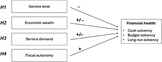
Therefore, a first hypothesis (H1) posits that service levels have a negative impact on financial health.
Economic wealth
The literature suggests local income is another external factor with a great impact. In their study of drivers for the financial condition of LG in Italy and Spain, Brusca et al. (2015) consider GDP and population size among others as “external determinants”.
Some scholars focus on trends in LGs’ tax base relative to their expenditures and commitments (Kloha et al., 2005), considering the gap between revenue capacity and expenditure as a cause of financial distress (Pagano and Moore, 1985; Inman, 1995). Local income per capita is an important indicator of the size of the tax base, which in turn has a positive effect on financial health (Capeci, 1991; Liu and Thakor, 1984). However, other studies find that while a strong tax base, often associated with a wealthier a community, can support financial health, it also relates with a higher demand for services (Bastida et al., 2013), which has a negative impact on financial health. Hence the second hypothesis (H2) is that economic wealth influences financial health positively/negatively.
Service demand
Demography is also an important factor outside a LG management domain, as population size is related to public service needs; on the one hand, the larger the LG, the greater is community demand (Capalbo and Grossi, 2014; Gardini and Grossi, 2018). On the other, larger cities, with higher resource levels, can optimize their organizational and management systems, leading to economies of scale and greater efficiency (Gomez et al., 2024). Hence, the third hypothesis (H3) posits that size may have either a positive or negative impact on financial health.
Fiscal autonomy
Gardini and Grossi (2018) identify several factors under LG control that affect financial health, such as local politics, mismanagement, culture, amalgamation strategies, budgetary practices, and transparency. Research finds that a higher capacity to generate revenue is associated with better financial health (Hendrick, 2011; McDonald and Maher, 2020) and that LGs face more financial risk when they rely on intergovernmental revenues because this causes uncertainty, as the decision-making power lies elsewhere (Chapman, 1988). Martell (2008) and Bastida et al. (2014) demonstrate that LGs having their own revenue have less debt, while other studies find a positive relationship between fiscal autonomy, defined as the proportion of revenues derived from locally generated resources, and financial health (Jones and Walker, 2007; Gomez et al., 2024), lowering the risk of default (Buendía-Carrillo et al., 2020). LG fiscal autonomy influences internal decision making, with Overmans and Timm-Arnold (2016) revealing that LGs’ level of control over their finances influences their reactions to financial crises; when LGs have greater control, they tend to use more fiscal leverage and cut expenditure less. Anessi-Pessina et al. (2012) find that fiscal autonomy negatively impacts capital expenses but not current expenditures. This aligns with the concept of cost stickiness, where resistance at the decision-making level hinders the reduction of current expenses despite decreasing demand or revenues (Cohen et al., 2017). Indeed, the proportion of own-source revenue may not fully capture fiscal autonomy (Ebel and Yilmaz, 2002). For instance, low own-source revenue does not necessarily distinguish between a LG that is heavily subsidized by the national government and one operating under a strong revenue-sharing or formula-based transfer system. In some cases, even when own-source revenues are low, LGs may still exercise significant discretion over expenditure decisions due to national regulations.
This reflects the broader and more complex debate on local autonomy, which encompasses multiple dimensions—including legal autonomy (formal status and powers), access (influence on higher-level decisions), policy scope (range of responsibilities), political discretion (decision-making authority), financial autonomy (control over revenues and expenditures), organizational autonomy (self-determination in structure and administration), and non-interference (freedom from higher-level oversight) (Ladner et al., 2023). Many of these aspects extend beyond the direct control of LGs, making the proportion of own revenues only one facet of the largest framework of fiscal autonomy.
Recognizing this limitation, this paper focuses exclusively on the internal factor of fiscal autonomy—measured as the proportion of revenues derived from locally generated resources. Accordingly, the fourth hypothesis (H4) posits that fiscal autonomy positively influences financial health, which serves as the central hypothesis of this study.
However, to maintain perspective and examine the relative importance of fiscal autonomy within the broader framework of the factors affecting financial health, Figure 1 provides all the four hypotheses outlined in the previous paragraphs. Regarding H2 and H3, the literature presents contrasting findings, with evidence supporting both positive and negative effects, reflecting its inherent ambiguity. In contrast, for H1 and H4, there is a consensus within the literature.
Methodology
To assess the influence of various factors on financial health, including the role of fiscal autonomy, a quantitative study was conducted using 2017 data from 269 municipalities in selected countries: Bosnia and Herzegovina, the Czech Republic, France, Italy, Portugal, Spain, plus Colorado and Virginia in the United States. These are countries with accrual or modified-accrual accounting to allow for data comparability. At the same time, they exhibit a medium to medium-high degree of local autonomy according to the Local Autonomy Index 2.0, which assesses the capacity of LGs to manage their affairs within a broader state framework independently (Ladner et al., 2023). Yet, these countries have diverse administrative systems, ranging from Napoleonic to Central European and Anglo-Saxon (Kuhlmann and Wollmann, 2019), which makes it useful for testing budget decisions in diverse settings, enhancing generalizability and suitable for hypothesis testing (Eisenhardt and Graebner, 2007; Seawright and Gerring, 2008). The diverse administrative systems selected ensure a variety of cultural and governance structures, aligning with previous comparative studies that aimed to analyze budget decision-making at the LG level (Padovani et al., 2024). Two US states are included as they have their own administrative structures, fiscal rules, and funding for LGs (Maher et al., 2023).
The largest municipalities in each country were selected. Each country had a minimum of 20 municipalities included, with the number expanded in cases where more data was available (see Appendix). The rationale for including the largest cities in each country is to ensure a certain level of comparability, as literature suggests that significant differences in public finance emerge between small and large cities (e.g. Czupich, 2020).
Data were collected by the Local Government Financial Sustainability Across Countries Group (LGFS-Across, 2025), a collaborative network aiming at standardizing financial information for cross-country comparison. The most recent comparable data available from official statistics is from accrual or modified-accrual accounting systems from 2017. LGs from countries with purely cash-based accounting standards could not be considered, as financial data would not have been comparable. Data from 2017 is interesting as it is sufficiently distant from the 2007–2008 global financial crisis and associated austerity programs (Geissler et al., 2019, 2021), but not yet affected by the 2020–2022 pandemic (WHO, 2023). Furthermore, World Bank reports (World Bank, 2018, 2019, 2020) indicate that 2017 was relatively stable economically and socially compared to 2018 and 2019. This stability allows for better control of factors that likely had a greater impact in 2018 and 2019.
Dependent and independent variables
Fiscal autonomy is the proportion of own revenues with respect to current revenues, while financial health is indexed through three main dependent variables, namely cash solvency, budget solvency and long-run solvency following the above literature. Cash solvency measures a LG liquidity and cash management, that is, its ability to pay off its short-term liabilities. In this study it is measured by the ratio between the cash ending balance and current expenditures. Hence, the higher the ratio, the more likely a LG can immediately pay off its short-term liabilities. Budget solvency refers to a LG ability to generate sufficient revenues to fund its current service levels, measured by dividing current revenues by current expenditures, in accrual terms and excluding depreciation. If it is below 1, there is a potentially dangerous imbalance. Long-run solvency refers to the impact of long-term obligations on current resources, that is a LG debt repayment capacity, calculated by dividing the year’s current revenues by the amount of long-term debt (loans) at the end of the year. The lower the ratio, the lower the risk that a LG would need to raise taxes or reduce services to pay its long-term debts or enter bankruptcy and risk state take-over proceedings.
As described in the literature review above, other variables that may influence financial health are the LG size, national context, level of economic wealth, and level of services offered. The main variables are outlined in Table 1.
Dependent and explanatory variables
| Variable type | Name | Description/formula |
|---|---|---|
| Dependent | Cash solvency | Cash ratio = cash ending balance/current expenditures |
| Budget solvency | Current balance = current revenues/current expenditures | |
| Long-run solvency | Debt repayment capacity = current revenues/non-current liabilities | |
| Main explanatory | Fiscal autonomy | % own revenues = own revenues/current revenues |
| Other explanatory | Size | Number of inhabitants |
| Economic wealth | Pro capita regional* gross local domestic product | |
| Service level | Pro capita current expenditures | |
| Dummies | Country | Nation with its rules and administrative traditions |
Regional = NUTS2, that is basic administrative areas for the application of regional policies that usually have between 800,000 and 3 million inhabitants
Analysis
The statistical analysis was carried out using different levels and types to ensure valid results (Greene, 2005). In the subsequent sections, univariate analysis will be used to describe various features of the data collected, while bivariate and multivariate analysis will be used to explore the relationship between fiscal autonomy and financial health. It is important to use various statistical tools to be able to extract complex and comprehensive messages from the data, which a single statistical technique may overlook or understate (Nielsen, 2018).
The analysis will be carried out in three phases.
An exploratory phase with descriptive univariate analysis of the data at hand to illustrate the main characteristics of the sampled LGs and bivariate analysis to verify correlations among the dependent and the independent variables.
A multivariate model with a multiple regression and a MANOVA to test the impact of fiscal autonomy on the three dependent variables (cash, budget, and long-run solvency), taking into consideration other explanatory variables.
A univariate model to verify the overall impact of fiscal autonomy on financial health through a simple linear regression model where financial health will be obtained through a principal component analysis of its three component variables.
This threefold approach provides insights from the data from different perspectives: first an overview about fiscal autonomy and financial health in the various municipalities across countries; then an investigation of the impact of fiscal autonomy on the three components of financial health, that is cash, budget, and long-term solvency; finally, an appreciation for the impact, if any, of fiscal autonomy on financial health as a single construct, acknowledging the role of other variables.
Findings
Phase 1 – fiscal autonomy and financial health: an overview
Table 2 shows the aggregate statistics for the sampled LGs, which range in size from a few thousand to a few million inhabitants, creating a heterogeneous sample that allows for effective assessment of the impact of population size on financial health. Fiscal autonomy varies greatly both across and within countries, as does average cash solvency. Conversely, average budget solvency is similar across most countries. Long-run solvency has the most variation across and within countries. The average service level by LGs is much lower in Bosnia and the Czech Republic and much higher in Virginia, and relatively similar across other countries but varies significantly within each country. The two US states have the most wealth, while Bosnia has the lowest. Between the two US states, Virginia has higher service levels and among European states, Bosnia has the lowest service level and economic wealth, while France’s is higher than that of Italy, Spain, and Portugal.
Descriptive results across countries
| BiH | CZ | FR | IT | PT | ES | CO | VA | Total | ||
|---|---|---|---|---|---|---|---|---|---|---|
| Sample size | 20 | 33 | 25 | 50 | 36 | 25 | 40 | 40 | 269 | |
| Size (inhabitants) | Mean | 38,305 | 74,748 | 330,295 | 292,792 | 97,485 | 510,662 | 94,193 | 69,351 | 181,9378 |
| Min. | 2,997 | 25,001 | 143,027 | 95,269 | 13,100 | 203,969 | 14,256 | 9,982 | 2,997 | |
| Max. | 199,191 | 382,405 | 2,265,886 | 2,856,133 | 508,209 | 3,223,334 | 717,632 | 459,470 | 3,223,334 | |
| Fiscal autonomy | Mean | 25.49% | 27.33% | 78.68% | 67.88% | 57.88% | 57.52% | 93.11% | 81.22% | 64.19% |
| Min. | 13.13% | 12.02% | 69.74% | 43.82% | 27.58% | 38.46% | 65.26% | 38.46% | 12.02% | |
| Max. | 43.17% | 50.64% | 86.81% | 94.31% | 81.44% | 70.67% | 100.00% | 93.41% | 100.00% | |
| Cash solvency | Mean | 8.41% | 84.23% | 11.00% | 25.45% | 27.41% | 25.85% | 56.96% | 35.82% | 36.50% |
| Min. | 0.45% | 9.49% | 1.39% | 0.00% | −7.86% | 3.26% | 13.53% | 3.52% | −7.86% | |
| Max. | 27.14% | 200.17% | 27.38% | 128.33% | 116.60% | 53.33% | 170.55% | 146.48% | 200.17% | |
| Budget solvency | Mean | 120.61% | 176.88% | 91.46% | 103.56% | 135.85% | 116.60% | 121.65% | 110.03% | 121.89% |
| Min. | 84.91% | 115.62% | 77.07% | 65.67% | 109.85% | 59.73% | 46.18% | 74.20% | 46.18% | |
| Max. | 152.68% | 268.37% | 121.19% | 123.01% | 185.44% | 138.59% | 243.28% | 138.68% | 268.37% | |
| Long-run solvency | Mean | 276.76% | 700.93% | 145.63% | 266.63% | 355.79% | 484.31% | 263.12% | 2078.05% | 618.77% |
| Min. | 61.13% | 69.21% | 48.51% | 29.80% | 66.30% | 103.81% | 40.73% | 443.71% | 29.80% | |
| Max. | 935.24% | 6326.24% | 486.41% | 2499.36% | 1442.39% | 3693.65% | 861.82% | 7645.56% | 7645.56% | |
| Service level € | Mean | 214.27 | 516.00 | 1210.64 | 1096.23 | 1011.53 | 899.61 | 902.84 | 1906.13 | 1032.17 |
| Min. | 128.84 | 355.93 | 776.89 | 584.29 | 292.06 | 628.62 | 294.18 | 440.52 | 128.84 | |
| Max. | 348.04 | 832.72 | 2061.77 | 2151.20 | 3210.42 | 1594.87 | 2554.05 | 4964.74 | 4964.74 | |
| Economic wealth € | Mean | 5,027* | 15,357 | 32,548 | 28,834 | 19,342 | 24,172 | 51,035** | 48,446** | 30,296 |
| Min. | – | 13,130 | 25,600 | 17,000 | 16,100 | 18,500 | – | – | 5,027 | |
| Max. | – | 17,157 | 58,100 | 45,000 | 31,400 | 34,100 | – | – | 58,100 |
Data not available as NUT2 not agreed upon; national data is used
Data are already based on the NUTS2 level
Source(s): Authors’ own work
The descriptive statistics reveal some counterintuitive findings. For instance, French LGs show high fiscal autonomy but the lowest debt repayment capacity, while Spanish LGs with lower fiscal autonomy exhibit better budget solvency and debt repayment. This implies that analyses should extend beyond national levels and that the relationship between fiscal autonomy and health may be more complex. Other variables may also play a significant role in explaining LG financial conditions, requiring further analysis.
Notably, the correlations among cash solvency, budget solvency, and long-run solvency are all positive and significant, supporting the assumption that they are positively related and the components of financial health (Table 3). The correlations among the three dependent variables and fiscal autonomy reveal that only budget solvency is significantly correlated with fiscal autonomy, while cash solvency and long-run solvency show no significant correlation, possibly even a negative one. Surprisingly, fiscal autonomy and budget solvency display a negative relationship, contradicting H4. This could suggest the presence of sticky costs (Cohen et al., 2017) or a higher focus on providing services for local development (Scutariu and Scutariu, 2015). These results require further analysis to explore the underlying relationship among the variables.
Bivariate correlation between dependent and main independent variables*
| Fiscal autonomy | Cash solvency | Budget solvency | Long-run solvency | ||
|---|---|---|---|---|---|
| Fiscal autonomy | Spearman’s ρ | – | |||
| Significance | – | ||||
| Cash solvency | Spearman’s ρ | 0.066 | – | ||
| Significance | 0.280 | – | |||
| Budget solvency | Spearman’s ρ | −0.383 | 0.426 | – | |
| Significance | <0.001 | <0.001 | – | ||
| Long-run solvency | Spearman’s ρ | −0.007 | 0.286 | 0.226 | – |
| Significance | 0.915 | <0.001 | <0.001 | – |
Significant relationships are italicized
Source(s): Authors’ own work
Phase 2 – the impact of fiscal autonomy on the components of financial health
A multivariate model was implemented with a multivariate multiple regression to estimate the impact of each explanatory variable on each dimension of financial health (Greene, 2005) and a MANOVA (multivariate analysis of variance) to assess the overall impact of different levels of fiscal autonomy on each dimension of financial health (Lipovetsky, 2015).
Multivariate multiple regression is used when two or more dependent variables are to be predicted from two or more independent variables, as in this case where the three components of financial health (cash solvency, budget solvency, and long-run solvency) need to be explained through fiscal autonomy, size, country, economic wealth, and service level.
The model was subjected to extensive diagnostic tests (Greene, 2005), and was found to satisfy basic regression model assumptions, particularly multicollinearity (strong correlation among independent variables) and heteroscedasticity (unequal variance). Multicollinearity was examined using variance inflation factors, which were found to be low for all explanatory variables in the model. The regression led to few significant results (shaded cells, Table 4):
Multivariate analysis – parameter estimates
| Dependent variable | Parameter | B | Std. error | t | Sig. |
|---|---|---|---|---|---|
| a. Cash solvency | Intercept | 0.153 | 0.072 | 2.128 | 0.034 |
| Fiscal autonomy | −0.175 | 0.152 | −1.148 | 0.252 | |
| Size | −3.467E−8 | 5.694E−8 | −0.609 | 0.543 | |
| Country | 0.071* | 0.009 | 8.353 | <0.001 | |
| Economic wealth | 2.248E−6 | 2.646E−6 | 0.849 | 0.397 | |
| Service level | 0.000 | 3.121E−5 | −3.854 | <0.001 | |
| b. Budget solvency | Intercept | 1.250 | 0.051 | 24.561 | <0.001 |
| Fiscal autonomy | −0.252 | 0.108 | −2.341 | 0.020 | |
| Size | 9.172E−9 | 4.032E−8 | 0.227 | 0.820 | |
| Country | 0.073* | 0.006 | 12.046 | <0.001 | |
| Economic wealth | −7.238E−6 | 1.874E−6 | −3.862 | <0.001 | |
| Service level | −4.941E−5 | 2.211E−5 | −2.235 | 0.026 | |
| c. Long-run solvency | Intercept | −2.714 | 2.172 | −1.250 | 0.213 |
| Fiscal autonomy | −5.672 | 4.596 | −1.234 | 0.218 | |
| Size | −2.409E−6 | 1.721E−6 | −1.400 | 0.163 | |
| Country | 1.033* | 0.258 | 4.002 | <0.001 | |
| Economic wealth | 0.000 | 8.000E−5 | 1.425 | 0.155 | |
| Service level | 0.004 | 0.001 | 4.097 | <0.001 |
Note(s): a. R Squared = 0.329 (Adjusted R Squared = 0.315)
b. R Squared = 0.542 (Adjusted R Squared = 0.533)
c. R Squared = 0.224 (Adjusted R Squared = 0.208)
Sign and value have no meaning
Source(s): Authors’ own work
The key variable influencing all three dependent variables is “country”, a dummy variable, supporting that the national context significantly affects financial health. As explained before, it is unimportant whether the effect is positive or negative, also because “country” is a nominal variable; what is relevant is that its effect is significant.
The second result indicates that service level negatively impacts budget solvency, confirming H1. Surprisingly, it positively affects long-run solvency, suggesting that offering more services pays off in the long term and aids debt repayment. Cash solvency is not significantly affected by the service level, likely due to contingencies. A third finding partly supports H2, as economic wealth negatively influences budget solvency, possibly due to increased demand for local public services (Bastida et al., 2013). The fourth outcome from the multivariate multiple regression analysis confirms the result of Phase 1 above and partly contradicts H4, as fiscal autonomy negatively impacts budget solvency. As mentioned before, this may be due to cost stickiness (Cohen et al., 2017) or greater pressure to provide services (Scutariu and Scutariu, 2015). LG size does not significantly impact any dimension of financial health, thus H3 is not supported as size does not have either a positive or negative impact on financial health.
The R-squared values indicating the model’s goodness of fit are low, particularly for cash and long-run solvency. While this is quite common in finance and accounting studies (Walker and Jones, 2006), it suggests the need for additional analysis to better explain these relationships. As some results appear controversial, a MANOVA (multivariate analysis of variance; Lipovetsky, 2015) was conducted with three subsamples of equal size for municipalities with low, middle, and high fiscal autonomy (Table 5).
Categorizing fiscal autonomy in three levels
| Fiscal autonomy | LGs | % | Cut off point for fiscal autonomy (own revenues/total current revenues) |
|---|---|---|---|
| Low | 90 | 33.5 | Lowest to 56.53% |
| Middle | 89 | 33.1 | 56.54–78.18% |
| High | 90 | 33.5 | 78.19% to highest |
| Total | 269 | 100.0 |
Source(s): Authors’ own work
The MANOVA (Table 6) shows whether there is statistical difference in the impact of levels of fiscal autonomy by LGs on their different solvency dimensions. For each couple of fiscal autonomy level, a significant result (cell marked in grey) would mean that the first level of fiscal autonomy has greater impact (whether negative or positive) on that solvency dimension with respect to the second level of fiscal autonomy. So, middle fiscal autonomy has a negative impact on cash and budget solvency with respect to low fiscal autonomy, but no significant effect on long-run solvency, while high fiscal autonomy has a negative impact on budget solvency with respect to low fiscal autonomy, but no significant impact on cash solvency and a positive effect on long-run solvency, and so on.
Multivariate analysis MANOVA ‒ contrast results (K matrix)
| Fiscal autonomy | Dependent variable | |||
|---|---|---|---|---|
| Cash solvency | Balance solvency | Long-run solvency | ||
| Middle vs. Low | Contrast estimate | −0.127 | −0.288 | −0.070 |
| Sig. | 0.017 | 0.001 | 0.962 | |
| High vs. Low | Contrast estimate | −0.032 | −0.317 | 4.355 |
| Sig. | 0.544 | 0.001 | 0.003 | |
| High vs. Middle | Contrast estimate | 0.095 | −0.028 | 4.425 |
| Sig. | 0.077 | 0.488 | 0.003 | |
Hence, first of all, results show that, contrary to H4 as for the regression analysis (Table 4), there is no significant linear relationship also between fiscal autonomy when grouped into levels and financial health, that is there is no common trend from low to middle to high fiscal autonomy which influences any of the three dimensions of financial health. Middle fiscal autonomy negatively impacts cash solvency more than low fiscal autonomy, suggesting that LGs with less autonomy are more cautious about their cash solvency, although this negative relationship is not significant for high vs. low fiscal autonomy. Moreover, low fiscal autonomy positively influences budget solvency more than middle or high autonomy, implying it is a better guarantor of balanced budgets. Lastly, high fiscal autonomy has a more positive impact on long-run solvency than low or middle autonomy, indicating that high autonomy helps pay off long-term liabilities. Overall, the MANOVA depicts a complex connection between fiscal autonomy and financial health.
Phase 3 – the impact of fiscal autonomy on financial health
The last phase of the analysis sought to verify whether fiscal autonomy has an overall impact on financial health (H4). To test this, we undertook principal component analysis on the three dependent variables, namely cash solvency, budget solvency, and long-run solvency, to investigate whether there is an underlying relationship among them and whether they can be brought back to a single variable, that is financial health.
The principal component analysis did extract only one component (Table 7), confirming one link underpinning the three variables. The Bartlett’s test of sphericity, the KMO measure of sampling adequacy, and the Cronbach’s Alpha coefficient of internal consistency confirm that the variables are related with some reliability, but there is a rather weak correlation with debt repayment capacity which does not really load with cash ratio and current balance, even though they are correlated two-by-two (Table 3). As the Cronbach’s Alpha coefficient was rather low (0.10) we first verified the coefficient without debt repayment capacity, which turned out to be 0.725, that is over the 0.7 threshold for consistency, and then we calculated the Average Variance Extracted (AVE) for convergent and discriminant validity and the composite reliability (CR) analysis for all three component values. Both were above the respective threshold of 0.5 and 0.7.
Principal component analysis ‒ component matrix
| Component | |
|---|---|
| Cash ratio | 0.885 |
| Current balance | 0.885 |
| Debt repayment capacity | 0.125 |
Note(s): Bartlett’s test of sphericity: approx. Chi-Square = 105.118, df = 3, sig. <0.001
Kaiser-Meyer-Olkin sampling adequacy = 0.502
Cronbach’s Alpha coefficient = 0.010, 0.725 without Debt repayment capacity
AVE = 0.527; CR = 0.717
The extracted component served as a single dependent variable in a univariate multiple regression with the same independent variables as in phase 2. Results in Table 8 show that multiple variables influence financial health, with a negative relationship between fiscal autonomy and financial health, contradicting H4. Service level significantly impacts financial health, but with no clear positive or negative direction. The regression R2 is around 50%, suggesting the model helps explain what influences financial health, but additional variables could provide a more comprehensive explanation.
Univariate linear regression – parameter estimates
| Parameter | B | Std. error | t | Sig. |
|---|---|---|---|---|
| Dependent = Financial health (component variable) | ||||
| Intercept | −0.339 | 0.175 | −1.934 | 0.054 |
| Fiscal autonomy | −0.787 | 0.371 | −2.120 | 0.035 |
| Size | −5.710E−8 | 1.390E−7 | −0.411 | 0.682 |
| Country | 0.256* | 0.021 | 12.264 | <0.001 |
| Economic wealth | −8.897E−6 | 6.460E−6 | −1.377 | 0.170 |
| Service level | 0.000 | 7.619E−5 | −3.294 | 0.001 |
Note(s): R Squared = 0.500 (Adjusted R Squared = 0.490), *Sign and value have no meaning
Discussion
This study explored the determinants of LG financial health, particularly the impact of LG fiscal autonomy on financial health. First, the analysis confirmed an underpinning relation among cash solvency, budget solvency, and long-run solvency, which are elements of financial health. Second, the analysis revealed the following in relation to the four hypotheses:
The service level has a negative impact on financial health: not corroborated.
Economic wealth influences financial health: partly corroborated.
Size influences financial health: not corroborated.
Fiscal autonomy positively influences financial health: partly corroborated.
The model did not really explore the characteristics of individual countries or whether the LGs of one country are more likely to be associated with cash solvency, budget solvency, and long-run solvency. The regression analysis simply revealed that national context is a key explanatory variable. As highlighted in the literature review, this may consist of factors such as institutional frameworks, fiscal rules, administrative and/or cultural traditions. Further studies would be needed to investigate which aspects of the national context influence financial health.
For H1 and H2, the analysis revealed that service level and economic wealth can influence financial health negatively because they may lead to unbalanced budgets. However, in the long run, they appear to positively influence financial health, likely due to a broader economic base for local taxes and fees (economic wealth). In fact, a higher level of expenditure may enhance the quality of public services, stimulating economic growth and generating higher public revenues. Additionally, domestic fiscal consolidation mechanisms may lead to higher service levels, which are more sustainable when municipalities maintain long-term financial health as a result (service level). However, municipalities with low economic wealth or low service levels may experience transient moments of financial health. Policymakers should be aware of this transience and consider providing sufficient structural support to ensure sustainable financial well-being.
Finally, concerning H4, we found that the relationship between LG fiscal autonomy and financial health is more complex than identified in previous studies that focus on long-term solvency or budget solvency in one country (Bastida et al., 2014; Carmeli and Cohen, 2001; Citro et al., 2018; De Matteis and Preite, 2018; Hruza, 2015; Kloha et al., 2005; McDonald and Maher, 2020; Martell, 2008; Padovani et al., 2018). Taking a multidimensional approach, our cross-national study found that the impact of fiscal autonomy on overall financial health is negative (Table 8), and particularly for cash solvency (Table 6) and budget solvency (Tables 3, 4 and 6). This is consistent with the outcome of H2 analysis (economic wealth positively influences financial health only in the long run), as there may be an interactive effect between economic wealth and fiscal autonomy, as greater community wealth could enable or encourage LGs to exercise higher levels of fiscal autonomy (Chapman, 1999).
Our analysis suggests that the complexity stems from the interaction between factors and contexts. First, fiscal autonomy positively influences short-term solvency only if it is low (Table 6) because lower fiscal autonomy corresponds to a reliance on resources provided by other public administrations (central, state, regional), more control from higher levels of government, and alleviation from the burden of local revenue collection. On the contrary, higher fiscal autonomy could be exploited by short-term interests, e.g. electoral support, which favor spending over meeting short-term obligations (Kloha et al., 2005). Second, fiscal autonomy needs to remain low not to have a negative effect on budget solvency (Tables 4, 6 and 8), because it brings an increased responsibility; if the level of fiscal autonomy crosses a certain threshold, LGs may struggle to efficiently allocate resources, resulting in an adverse impact on the delivery of essential services, increased expenditures, and undermining budget solvency (Jimenez, 2020). Third, there is an optimal high level of fiscal autonomy associated with long-term solvency (Table 6); a high level of fiscal autonomy generates greater accountability in the medium to long term so LGs relying on their own resources have greater responsibility for financial health in the long term.
Hence, our study extends the existing literature in finding that, while a high level of fiscal autonomy appears to be beneficial for long-term solvency, it can pose challenges for short-term solvency and budget stability, generating a possible negative impact on overall financial health. Our analysis reveals that prior research on the impact of fiscal autonomy on the financial viability of LGs has often taken a too narrow view and has significantly underestimated the importance of temporal dynamics in public policymaking and management. This is in line with Martell and Moldogaziev (2023), who emphasized that LGs have to make choices in how they use their resources, and thus there are trade-offs in funding current, capital, and debt servicing expenditures, with different implications in the short and long run. The concept of financial health is not independent of time; rather, it is a multidimensional concept with short, middle, and long-term dimensions, that is, cash solvency, budget solvency, and long-run solvency, respectively.
Therefore, while NPM emphasizes fiscal autonomy as a means to enhance the management of public resources (Hood, 1991, 1995; Pollitt, 1993; Dunleavy and Hood, 1994; Ferlie et al., 1996; Mussari, 1996), our study reveals that the situation is more complex. The components of financial health may serve different, sometimes competing, purposes, with a time-oriented perspective being crucial. For instance, long-term solvency provides LGs the flexibility to invest in new infrastructure without jeopardizing short-term financial stability. A strong budget solvency enables LGs to absorb unexpected shocks, such as revenue declines from economic downturns, cost increases from inflation, or the need to ramp up services during crises like natural disasters. Similarly, good cash solvency ensures timely payments, preventing service interruptions and avoiding costs associated with delayed payments. National policymakers and local officials must carefully balance financial autonomy with the need to maintain immediate financial health, ensuring sustainable growth, addressing current community needs, and preserving long-term fiscal resilience. When a LG has a high level of fiscal autonomy, there should be a greater focus on short-term solvency and budget solvency, while when an LG relies on subsidies received from other entities, emphasis should be placed on long-run solvency. Nevertheless, policymakers and local officials should consider the broader concept of fiscal autonomy (Ebel and Yilmaz, 2002) and in general local autonomy (Ladner et al., 2023), where the share of own revenues represents just one lever.
Conclusions
This study adds to the debate on local finances at a cross-country level by investigating the relationship between fiscal autonomy and financial health, finding that the relationship is more complex than the linear and positive relationship identified by previous literature (Hendrick, 2011; McDonald and Maher, 2020). Our research contributes to the literature in two further ways. First, it introduces a method that compares LGs across countries through a reclassification of financial information produced by different accounting systems, overcoming the absence of widely accepted and uniform international standards. Second, undertaking a cross-country analysis reveals that despite diversity across national contexts, some global patterns have emerged with the promotion of global accounting standards like accrual and IPSAS (Polzer et al., 2021). The main finding is that there are no linear relationships between fiscal autonomy and financial health. Fiscal autonomy correlates positively with financial health in the long-term, but negatively in the short-term, considering either cash or budget solvency. This might be due to the imposition of controls by higher levels of government that may cause a better governance of local public finances than self-government mechanisms (Sutherland et al., 2018). Thus, decision makers at national as well as local level should take these intertemporal relationships and trade-offs into consideration in their efforts to enhance local governance and financial health. For policy makers, the study highlights the need for targeted interventions and tailored policies that account for the varying temporal impacts of fiscal autonomy. Training programs, institutional reforms, and financial and administrative support mechanisms can mitigate the short-term risks while enabling LGs to realize the long-term benefits of fiscal autonomy. On the supranational policy side, our findings suggest that promoting international standards such as accrual accounting and IPSAS could foster comparability and transparency across LGs, supporting better governance and accountability practices.
Our study, therefore, has benefited from a more comprehensive approach to financial health by introducing a temporal perspective and emphasizing its crucial role in determining the effects of fiscal autonomy. Using more than one statistical technique has made it possible to obtain more robust results and to explore some nuances that any analysis carried out in isolation might not have revealed. However, as with any statistical analysis, causal relationships and empirical analysis do not provide definitive evidence, answers, or explanations. Further analysis should be carried out on a larger sample, including more LGs and more countries, and over a longer period to verify our findings. Also, the research could cover only LGs in countries with accrual or modified-accrual accounting standards. LGs in countries with a purely cash-based system had to be excluded from our sample so that separate research could be conducted for them. Moreover, there could be additional factors to consider, which future research may explore, potentially rooted in individual countries’ cultural or political context, such as the broader concept of fiscal and local autonomy—factors that go beyond strictly financial dimensions and are not captured by financial data alone yet are operationalizable across countries. These aspects remain critical for understanding the broader implications of fiscal autonomy on LG.
We acknowledge the valuable contributions of the country experts involved in the Local Government Financial Sustainability Across Countries (LGFS-Across) Group, a collaborative network dedicated to standardizing financial information for cross-country comparison, who provided us with the financial dataset used in this study (https://site.unibo.it/LGFS-Across).
Appendix
LGs by country
| Bosnia and Herzegovina | Czech Republic | France | Italy | Portugal | Spain | Colorado, USA | Virginia, USA |
|---|---|---|---|---|---|---|---|
| Banja Luka | Tábor | Aix en provence | Torino | Almada | Madrid | Denver | Alexandria |
| Prijedor | Cheb | D’angers | Novara | Amadora | Barcelona | Colorado Springs | Blacksburg |
| Foča | Karlovy Vary | Bordeaux | Genova | Aveiro | Valencia | Aurora | Bristol |
| Nevesinje | Česká Lípa | Brest | Milano | Barcelos | Sevilla | Fort Collins | Charlottesville |
| Istočno Novo Sarajevo | Jablonec nad Nisou | Clermont Ferrand | Bergamo | Beja | Zaragoza | Lakewood | Chesapeake |
| Pale | Liberec | Dijon | Brescia | Braga | Málaga | Thornton | Christiansburg |
| Oštra luka | Most | Grenoble | Bolzano | Braganca | Murcia | Arvada | Colonial Heights |
| Novi grad | Hradec Králové | Le Havre | Trento | Cascais | Palma de Mallorca | Westminster | Culpeper |
| Kneževo | Pardubice | Lille | Verona | Castelo Branco | Las palmas | Pueblo | Danville |
| Kotor varoš | Trutnov | Lyon | Vicenza | Coimbra | Alicante | Greeley | Fairfax City |
| Čelinac | Zlín | Marseille | Venezia | Evora | Córdoba | Boulder | Falls Church |
| Ugljevik | Jihlava | Montpellier | Padova | Faro | Valladolid | Centennial | Fredericksburg |
| Bileća | Třebíč | Nantes | Udine | Funchal | Vigo | Longmont | Front Royal |
| Trebinje | Uherské Hradiště | Nice | Trieste | Gondomar | Gijón | Loveland | Hampton |
| Šipovo | Znojmo | Nimes | Piacenza | Guarda | Hospitalet de llobregat | Broomfield | Harrisonburg |
| Teslić | Frýdek-Místek | Reims | Parma | Guimaraes | Granada | Castle Rock | Herndon |
| Mrkonjić Grad | Třinec | Rennes | Reggio Emilia | Leiria | A coruña | Grand Junction | Hopewell |
| Laktaši | Havířov | Saint Denis | Modena | Lisboa | Elche | Commerce City | Leesburg |
| Šamac | Karviná | Saint Etienne | Bologna | Maia | Terrassa | Parker | Lynchburg |
| Bijeljina | Orlová | Strasbourg | Ferrara | Matosinhos | Badalona | Littleton | Manassas |
| Olomouc | Toulon toulouse | Ravenna | Odivelas | Oviedo | Brighton | Manassas Park | |
| Opava | Villeurbanne mans | Cesena | Oeiras | Cartagena | Northglenn | Martinsville | |
| Přerov | Paris | Forli’ | Ponta delgada | Sabadell | Englewood | Newport News | |
| Šumperk | Ancona | Portalegre | Móstoles | Windsor | Norfolk | ||
| Ostrava | Firenze | Porto | Santa Cruz De Tenerife | Wheat Ridge | Petersburg | ||
| Brno | Livorno | Santa Maria Da Feira | Erie | Poquoson | |||
| Arezzo | Santerem | Lafayette | Portsmouth | ||||
| Perugia | Seixal | Fountain | Purcellville | ||||
| Terni | Setubal | Evans | Radford | ||||
| Roma | Sintra | Louisville | Richmond City | ||||
| Latina | Viana Do Castelo | Montrose | Roanoke City | ||||
| Giugliano in Campania | Vila Franca De Xira | Golden | Salem | ||||
| Napoli | Vila Nova De Famalicao | Durango | Staunton | ||||
| Salerno | Vila Nova De Gaia | Johnstown | Suffolk | ||||
| Pescara | Vila Real | Canon City | Vienna | ||||
| Foggia | Viseu | Firestone | Virginia Beach | ||||
| Bari | Greenwood Village | Warrenton | |||||
| Taranto | Frederick | Waynesboro | |||||
| Lecce | Federal Heights | Williamsburg | |||||
| Reggio Calabria | Lone Tree | Winchester | |||||
| Palermo | |||||||
| Messina | |||||||
| Catania | |||||||
| Siracusa | |||||||
| Sassari | |||||||
| Cagliari | |||||||
| Rimini | |||||||
| Prato | |||||||
| Monza | |||||||
| Andria |
Source(s): Authors’ own work

