Assigning Eurozone sovereign credit ratings using CDS spreads

It became evident during the credit crisis of 2008 that there were several major issues with sovereign credit ratings issued by the Big 3 (S&P, Moody’s and Fitch). The main issues were a misuse of their position, as they control 95 per cent of the market (Klein, 2004; Eijffinger, 2012; Taylor et al., 2011), a conflict of interest (EC, 2013; Larosiere et al., 2009; Ozturk et al., 2016), not being transparent about the rating procedure (Iyengar, 2010; Katz et al., 2009; Benmelech and Duglosz, 2009) and a slow response to market changes (Eijffinger, 2012; Ozturk et al., 2016). Due to these issues, the sovereign credit ratings that were issued did not reflect the true credit risk faced by a sovereign adequately.

Take Iceland for example – prior to September 29, 2008 – was considered to be relatively credit worthy, as evidenced by the credit ratings issued by the Big 3 (Table I). According to these ratings, Iceland should have had enough liquidity to withstand a mild to severe crisis. However, within just three days, the three major banks of Iceland defaulted on $62bn dollars of external debt and were nationalized by the government (Amadeo, 2015). It is remarkable that the credit ratings for Iceland were positive just the day before the crisis started, as the external debt of Iceland in June 2008 was seven times the GDP of 2007 (Iceland Statistics, 2008). As a comparison, the ratio of debt (both internal and external) to GDP in the USA in 2013 was 1.045 (IMF, 2014). At that time, the USA was rated AAA by Moody’s (2013), which was just one step above the rating that was assigned by Moody’s for Iceland before the crisis. As a result of the chaos that occurred, the Króna lost 50 per cent of its value against the US dollar in just one week (Central Bank of Iceland, 2008), the stock market fell 95 per cent (Amadeo, 2015) and many businesses went bankrupt (Anderson, 2015). After nationalization, the credit ratings agencies had to downgrade Iceland to keep up with the current situation (as can be seen in the second column in Table I). This revision, however, came too late. This example highlights the relevance of sovereign credit ratings and the need for these to be issued in a rigorous manner.

In this paper, we propose a novel framework that uses credit default swap (CDS) spreads to estimate the probability that a sovereign will default. A CDS is essentially an insurance contract that the buyer of a bond (sovereign or corporate) purchases. The seller of the CDS agrees to pay to the buyer a portion of the bond’s face value in the event that the sovereign or corporate experiences a default event. In exchange for this insurance, the buyer makes a sequence of payments to the seller. This payment or premium is termed as the CDS spread and is usually expressed in basis points with reference to the nominal amount of the swap. The CDS market is a highly liquid market (Ang and Longstaff, 2013). Changes in the CDS spreads can therefore quickly signal changes in the creditworthiness of the corporate or sovereign underlying the bond.

Our framework uses the multi-factor affine model developed by Ang and Longstaff (2013) to study sovereign credit risk of Eurozone countries using CDS spreads. This model allows for both systemic and sovereign-specific credit shocks but is not forward looking and can only be used in a retrospective study. To be able to investigate the current situation, financial and macroeconomic data can serve as proxies for the current health of a sovereign’s economy and be used as indicators of future performance. As mentioned by Ang and Longstaff (2013), there is a certain relationship between sovereign credit risk and macro-economic and financial variables, which has to be explored. This is further explored in this paper. Our framework therefore retains the focus on systemic and sovereign-specific credit shocks of the Ang and Longstaff (2013) model and extends it by incorporating a regression model on indicative financial and macroeconomic variables. We calibrate the framework using data from 2007 to 2010 and test it during the peak of the sovereign debt crisis (2010 to 2013). Our framework results in a better estimation of the default risk as compared to the model by Ang and Longstaff (2013), as seen in Table IV. With the framework, we can estimate the probability that a sovereign will default on its debt. These default probabilities can then be used to assign credit ratings to sovereigns. We illustrate the framework on eight Eurozone countries and show that the ratings assigned by our framework are both accurate and responsive to market changes. In comparison to the ratings assigned by the Big 3 (Section 5), our framework is able to provide an early warning on the change in the creditworthiness of a sovereign, whereas the Big 3 are slow to respond to the market. Further-more, by using default probabilities to assign sovereign credit ratings, our framework provides transparency (in contrast to the ratings assigned by the Big 3). We emphasize that while the framework is presented in the context of the eight Eurozone countries, the framework itself is generic and can be easily applied to data from other countries with minor modifications. The accuracy and responsiveness of our framework further imply that when assessing the systemic and idiosyncratic risks of sovereigns, both macroeconomic and financial factors must be considered.

The paper continues with a brief literature review in Section 2. We provide an explanation of the data used in Section 3 and the model description in Section 4. The alternative ratings procedure and the comparison with the ratings issued by the Big 3 are explained in Chapter 5 and the paper concludes in Section 6.

Our work is primarily related to the literature on assessing sovereign credit risk. More specifically, we contribute to the literature on assessing sovereign credit risk using CDS spreads.

To address the shortcomings of the ratings issued by the Big 3, several models have been developed to assess sovereign credit risk. Much of the recent literature works on assessing sovereign credit risk have focused on European sovereigns, given the euro debt crisis which started in 2009, when Greece became the first European sovereign to face financial problems (Gibson et al., 2014). Other countries followed, such as Ireland, Portugal, Spain and Italy; these countries are collectively known as the PIIGS countries. The Eurozone continues to be volatile given recent political and economic conditions. As such, assessing the sovereign credit risk of countries in the Eurozone remains a priority. One approach to assessing sovereign credit risk is the development of a statistical model using historical default data to build an empirical distribution of the probability of default. Given the limited number of sovereign defaults in Europe to date (Reinhart and Rogoff, 2008) and differences between the definitions of default in each case, the potential of a statistical model using historical default data to assess sovereign credit risk is rather restricted.

Gibson et al. (2014) stated that there are two main alternatives that one can use to assess sovereign credit risk. The first alternative is the use of sovereign bond yields. If the yield increases, one would assume that the level of sovereign credit risk increases. The second alternative is to use the CDS spread, which reflects the implied market perception of sovereign credit risk. The CDS market is more liquid than the sovereign bond market (Pan and Singleton, 2008). Furthermore, the CDS spread is a direct measure of implied sovereign credit risk, whereas bond spreads are also subject to interest rate risk (Ang and Longstaff, 2013) and liquidity risk (Longstaff et al., 2005). Consequently, the usage of the CDS spreads to assess sovereign credit risk would better reflect the true credit risk of a sovereign. Kiesel and Spohnholtz (2017) also argued that CDS spreads are better indicators of credit risk and demonstrated the use of CDS data on corporate bonds to issue credit ratings for corporations.

Within the work so far conducted on using CDS models to assess sovereign credit risk, there is a classification into two different types of models. The first category consists of models that split the CDS spread into a default and risk premium part. The default part is the share of the spread that represents the implied default probability, whereas the risk premium part can be seen as the implied market value. The advantage of this model is that it is capable of deriving a clear implied sovereign credit risk default value, but not what the factors are that change this value. Examples of such models can be found in articles by Pan and Singleton (2008), Longstaff et al. (2011) and Duffie and Singleton (2003). The second category consists of models that split the CDS spread into a systemic risk part, which affects each borrower, and an idiosyncratic risk part, which is sovereign specific. This type of model provides a more in-depth analysis of what drives sovereign credit risk and more specifically, to what extent it is dependent on the status of other sovereigns. There are a limited number of articles available in this category, but an example of such a model can be found in Ang and Longstaff’s study (2013). As there is a lot of debate going on in Europe whether sovereign credit risk is mainly affected by other sovereigns and the second type of model is capable of splitting the implied sovereign credit risk into a systemic and idiosyncratic risk part, the second type of model is preferred to be used in the current economic condition.

The model that was tested by Ang and Longstaff (2013) (henceforth: AL-CDS model) is quite accurate when one looks back over the period till the euro debt crisis. The AL-CDS model has a backward looking design, and its performance for future prediction is not clear. It would be interesting to measure its performance on the data of the euro debt crisis. The model is solely based upon the CDS spread and does not take into account financial and/or macroeconomic data for the calculation. However, the authors investigate the relationship between systemic risk and financial factors, finding that there is a significant relationship. They also mention that more attention has to be paid to this relationship, since they test a limited set of financial variables and other financial variables could provide more insight. Furthermore, several researchers point out that one should include macroeconomic variables if one investigates the euro debt crisis (Gibson et al., 2014; Afonso et al., 2014; Bernoth et al., 2012; Hagen et al., 2011). As the model is retrospective in nature and does not include financial and/or macroeconomic data for the calculation, the question arises whether the model is accurate for future predictions and specifically when one tries to model the euro debt crisis. To provide an answer to this question, this research tries to identify whether the AL-CDS model can be used for future predictions and whether incorporating financial and/or macroeconomic date results into a more accurate model for future predictions. Based upon this model, a sovereign credit risk rating scale can be designed which can replace the current rating procedure used by the Big 3.

Our investigation covers the period from April 2007 to April 2013. We collect the CDS spreads, and financial and macroeconomic data over this time period for eight countries in the Eurozone. We split the six-year time span in to a calibration period and a testing period. The calibration period is set to 3.5 years, from April 2007 to September 2010. The model parameters obtained from the calibration are tested on the remaining 2.5 years of data. Below we discuss some characteristics of the collected data.

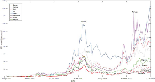
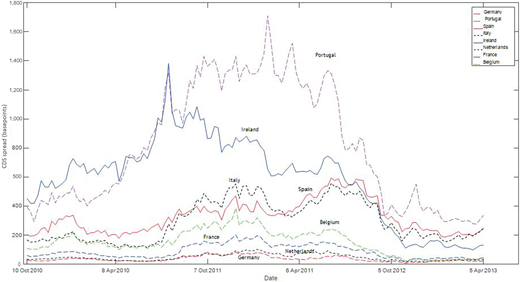
We collect the one- and three-year CDS spreads of eight sovereigns in the Eurozone from Bloomberg. The eight countries are Germany, Netherlands, France, Belgium, Italy, Spain, Ireland and Portugal. This choice allows us to perform an in-depth analysis in the Eurozone, as we cover sovereigns having less fluctuation in their CDS spread (such as Germany) and those that have a high fluctuation in their CDS spread (such as Portugal). We are also able to analyze the dependency of a sovereign’s credit risk on its own performance and macroeconomic variables, as well as other sovereigns. Greece has not been included in our data set as the CDS spread of both the three-year and five-year maturity is extremely high (over 30,000 basis points). The three-year maturity CDS spread for the calibration period can be seen in Figure 1 and for the testing period in Figure 2.

We would like to note certain observations regarding the data. There is no data available on Ireland’s CDS spreads before the first of January 2008, when they started to issue CDS contracts. Ireland has the highest CDS values for the calibration period (a mean of 143 basis points and a maximum of 470 basis points), whereas Portugal has the highest values for the testing period (a mean of 807 basis points and a maximum of 1,711 basis points). A high CDS value reflects a high level of sovereign credit risk. For all the European sovereigns, we see an increase in the CDS spread from 2010, which marks the start of the euro debt crisis. We also remark that among the eight countries under consideration, Portugal has the highest standard deviation due to the high fluctuation in its CDS spread. It is of interest to note that for both Portugal and Ireland, the 3-years CDS spread is higher than the 5-years CDS spread for about a third of the time span. This is why we do not include the 5-year spread in our calibration and testing.

During the testing period, the CDS spread is much higher compared to the calibration period for all sovereigns. Portugal and Ireland still show the reverse behavior with the three- and five-year maturity CDS spread. Germany continues to have the lowest CDS spreads and is thus perceived to have the lowest level of implied sovereign credit risk. We see that for all the countries, the highest CDS spread was in 2011 which marks the peak of the euro debt crisis. From 2012, a downward trend in the CDS spreads is observed for all the sovereigns, implying that the level of sovereign credit risk starts to diminish.

The systemic risk component of the sovereign risk is calibrated with many financial factors. Many articles show, as well as point, the need to establish this relationship, such as those of Wegener et al. (2016), Rösch (2003), Ang and Longstaff (2013), Jakubík (2006), Hamerle and Liebig (2003), Koopman et al. (2012) and Virolainen (2004). These articles provide us a comprehensive list of financial variables to use. In addition, we use corporate financial data as they are highly correlated with the performance of the country and also because limited information is available on the factors for sovereigns. The following variables were collected from Bloomberg:

• FX rates (Euro-Dollar ratio, Euro-Pound ratio, Euro-Yen ratio, Euro-RMB ratio);

• Stock indices (NASDAQ index, S&P500 index, Eurostoxx index);

• VIX indix (EU VIX Eurostoxx);

• Commodities (Brent Oil price per barrel in Euro, Gold price per ounce in Euro);

• Bond prices (one-, three- and five-year Euro-bond bid prices);

• Swap rates (one-, three- and five-year swap rates); and

• Interest rates (one-, three- and six-month Euribor, ECB interest rate, Euro-Dollar deposit interest rate, TED Spread, LIBOR-OIS spread).

The FX rates are the ones used in the IMF basket of the Special Drawing Rights valuation. The US stock indices are included as the USA is the biggest economy in the world and the biggest trading partner of the European Union (Directorate General for Trade, 2016). The VIX index has been included as it is a strong indicator for systemic risk, as mentioned by Ang and Longstaff (2013). The oil price has been included since it has been shown by Wegener et al. (2016) that positive oil price shocks lead to lower sovereign CDS spreads. The bond prices, swap rates and interest rates have been selected using a combination of several frameworks (Rösch, 2003; Ang and Longstaff, 2013; Jakubík, 2006; Hamerle and Liebig, 2003; Koopman et al., 2012; Virolainen, 2004).

A selection of 14 financial and macroeconomic variables has been made to assess the idiosyncratic (or non-systemic) sovereign credit risk. We chose these variables as they are valid indicators of idiosyncratic risk for sovereigns, as well as corporate institutions, as mentioned by Koopman et al. (2012), Rösch (2005), Jakubík (2006) Hilscher and Nosbusch (2010) and Gestel et al. (2006). The data are collected from Bloomberg, ECB and Eurostat at a sovereign level. The variables collected are:

• finance (10-year treasury bond bid price, stock index, interest rate on deposits, long-term interest rate, inflation ratio);

• unemployment ratios (total unemployment, unemployment over 25 years, unemployment under 25 years);

• industry indices (production index construction, manufacturing turnover index); and

• balances (real effective exchange rate, international trade ratio, index of deflated turnover), economic indices (Generic economic situation over the next year of customers, financial situation over the last year of customers).

No data are available for the production index construction for both Ireland and Spain.

In this section, we first explain the backward looking model developed by Ang and Longstaff (2013), which forms the base of our framework and model. We calibrate it using data from 2007 to 2010 and test its performance on data from 2010 to 2013. Seeing the deficiencies in the AL-CDS model’s performance, we develop an alternative model, explained in Section 4.2.

The AL-CDS model is based on the classical framework presented by Duffie and Singleton (2003)[¹]. The model assumes two kinds of shocks – a systemic shock that affects every sovereign and a non-systemic shock (or idiosyncratic shock) that only affects the default probability of an individual sovereign. The systemic and non-systemic shocks are assumed to be independent of each other. The idiosyncratic shock is the same as the underlying standard reduced-form credit models used by (Pan and Singleton, 2008; Duffie and Singleton, 1999). In the AL-CDS model, the idiosyncratic default is triggered by “the first jump of a sovereign-specific Poisson process” (Ang and Longstaff, 2013). This intensity process follows a standard square-root process for sovereign i:

where a_i, b_i and c_i are constants and Z_i,t is a standard Brownian motion, all sovereign specific. The constants a_i, b_i and c_i denote the slope and curvature of the idiosyncratic part of the CDS term structure (or a_i represents the mean, b_i the rate of adjustment towards the mean and c_i the volatility), whereas the values of ζ_i,t reflect the idiosyncratic risk level of the CDS spread of a sovereign. This setting allows for mean reversion and conditional heteroskedasticity in the intensity process and guarantees that the intensity process never becomes negative. It has to be noted that there is no restriction placed on the correlation between the Brownian motions across sovereigns, as this is partially taken into account by the systemic risk intensity process (except for Germany, which we assume has no idiosyncratic risk).

Systemic risk affects every sovereign, but each sovereign experiences its impact differently. This impact is modeled by the parameter γ_i which is sovereign specific and is assumed to be constant. The intensity process for systemic risk is also modeled as a Poisson intensity process, which follows a standard square-root process:

where α, β and σ are constants and Z_λ,t is the Brownian motion of the systemic risk intensity process in equation (2). The constants α, β and σ denote the slope and curvature of the systemic risk part of the CDS term structure (or α represents the mean, β the rate of adjustment toward the mean and σ the volatility), whereas the value of λ_t reflects the systemic risk level. The Brownian motion for systemic risk and the Brownian motions driving the idiosyncratic risk are uncorrelated. Similar to the idiosyncratic risk intensity process, the systemic risk intensity process can never become negative. The probability that there is no default of sovereign i by time t can be expressed as follows:

The total default intensity is the sum of the idiosyncratic shock intensity ζ_i,t and the systemic risk intensity λ_t multiplied by the exposure (or impact) γ_i. Sovereign credit risk thus depends on the two intensity processes and the exposure. These values can be derived from the CDS spread (s_i,t,τ) of sovereign i and maturity τ using the following formula:

where ω is the recovery rate and D(t, τ) is the value of a risk-free zero-coupon bond with maturity τ at time t. The formulas for A(λ, t), B(ζ_i, t), C(ζ_i, t), F (λ, t) can be found in the appendix and have been derived by Ang and Longstaff (2013). The value of ω has been set at 50 per cent, which is in line with Duffie and Singleton (2003) and Ang and Longstaff (2013). The recovery rates are usually in the range of 30 to 75 per cent, as shown in Sturzenegger and Zettelmeyer’s study (2008). The value of ω will have little effect on the estimates of the systemic and idiosyncratic components since it is applied to both legs of the CDS contract in the estimation process. If this rate varies over time, it can have an impact on the spreads without a big movement in the systemic risk component. Therefore we also assume here that the recovery rates are constant over the time period in consideration[²].

A sovereign default event is assumed to occur upon the first arrival of either of the two Poisson processes, but in reality a default is triggered by credit events described in the CDS contracts. The precise legal definition of a sovereign default is thus not fully captured by the model. We work with the risk-neutral measure, since there are almost no historical cases of sovereign defaults. We take the country with the lowest CDS spread to be the comparison country - and its default depends only on systemic risk. In this paper, Germany is set as the comparison country since it has the lowest CDS spread, in addition to being the biggest economy in the Eurozone.

The constants and the intensity processes have been estimated using the one- and three-year CDS spread over the calibration period. We chose to exclude the five-year CDS spreads as there were many instances when the five-year spread was lower than the three-year spread. The values for the zero coupon bonds D(t) have been bootstrapped using the one-, three- and six-month Euribor rates and the one-, three and five-year swap rates, collected from Bloomberg. The cubic spline interpolation algorithm (Longstaff et al., 2005) has been used to calculate these values. The recovery rate is set to ω = 0.5, which is in line with Ang and Longstaff (2013) and Lando (1998). The parameters are estimated using the nonlinear least squares method:

where s_i,t,τ denotes the CDS spread of issuer i of maturity τ at time t, and sˆ_i,t,τ is the estimated CDS spread calculated using equation (4) where λ, ζ₁, …ζ_N represent the systemic and idiosyncratic risk intensities and θ represents the vector of the estimated parameters α, β, σ, a_i, b_i, c_i and γ_i.

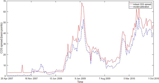
As Germany is the country that represents systemic risk in the Eurozone, the systemic risk constants α, β, σ and the systemic risk intensity values λ_t have been estimated first, over data of Germany. Note that γ_Germany = 1 as Germany is the base for systemic risk. The second step is to estimate the constants a_i, b_i, c_i, γ_i and the idiosyncratic risk intensity process ζ_i,t for each of the seven sovereigns. Further details of the calibration steps can be seen in Ang and Longstaff’s study (2013). The outcome of the calibration of the parameters can be found in Table II, in which the standard error is listed within brackets and the RMSE is denoted in basis points. As can be seen, the model has a good fit to the term structure of the CDS spreads. The RMSE values for each country are between 6 and 21 basis points, a small percentage of their absolute CDS spreads. To illustrate the fit, the outcome of the calibration for France for the one-year maturity in shown in Figure 3.

The AL-CDS model was designed for backward calculation and does not perform well for future prediction (see Section 4.3). It needs to be re-calibrated every time the default probability needs to be calculated. To improve on the predictive power, we present a regression-based model – referred to as Reg-model hereafter. A reliable estimation for λ and ζ is important since they are the key components to calculate the survival probability, as can be seen in equation (3). Based upon these two intensity process values, the default probability can be estimated for each sovereign. Given the intensity process values λ and ζ, a regression analysis of the relevant financial and macroeconomic variables has taken place to reveal the relationship. Given that there are a high number of explanatory variables, a factor analysis has been executed to identify which variables are independent and able to explain the major share of the variance. These variables are used as input for the regression model. The model’s performance is observed over the testing period and the results can be seen in Section 4.3. Note that the number of independent variables, n and m, in the regression outcome may vary by sovereign:

For each of the sovereigns, we conduct a factor analysis using an orthogonal rotation technique (Varimax). A factor analysis reveals what factors explain the major share of the variance, while keeping in mind that the factors are not correlated to eliminate multicollinearity. The outcome of the factor analysis is reported in the  Appendix and reveals what variables can be used as input for a regression analysis. Based upon the several explanatory variables that are independent, different models for each country have been tested using lagged time series. The model with the highest R-square value has been selected as the final model for each sovereign. Note that each sovereign has a different model, given that the Reg-model allows a differentiation on sovereign level. A summary of the outcome can be seen in Table III, whereas more detailed information is reported in the  Appendix (with lags, t-stats, etc.).

As can be seen, the R-squared values are between 0.662 and 0.845, which indicates that a significant portion of both the systemic risk and the idiosyncratic risk intensity process can be explained by financial and macroeconomic data. More information about the outcome of the regression analysis can be found in the Appendix (such as the lag on a variable, t-statistics, etc.), in which is also shown that all variables are significant at a 99 per cent level. Based upon the estimate for each explanatory variable, the values of λ and ζ can be estimated for the testing period. These estimated values are used as input for the default probability calculation.

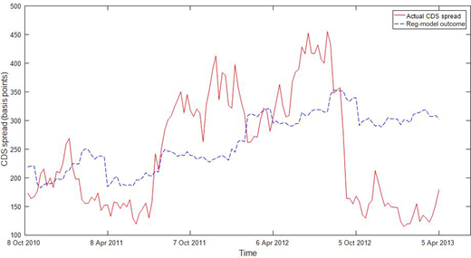
Based upon the settings for the AL-CDS model and the Reg-model, the CDS spreads of both the one-year and three-year maturity have been simulated for the testing time period. Note that the actual data of the macroeconomic variables over the testing period have been used, in which the estimated λ and ζ values are used as input for the CDS spread calculation. The RMSE between the actual and the estimated CDS spread from the models is shown in Table IV. We can conclude that the Reg-model does better than the AL-CDS model (it has a lower RMSE), as it incorporates the financial and macroeconomic data. The smallest RMSE values can be found for the country with the lowest CDS values, which is Germany with a RMSE value of 14 basis points. The highest RMSE values are for Portugal and Ireland, the countries with the highest CDS spread. Thus, the Reg-model can be used for forecasting, which is necessary to assign a credit rating for a sovereign.

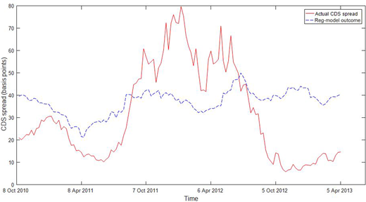
The outcome for two different countries for the one-year maturity is shown in Figures 4 and 5. As can be seen in these figures, the Reg-model yields an accurate fit for the first two years, while it does not incorporate the decrease of the CDS values in the last half year. This is due to the fact that there is no significant change in the macroeconomic data for the last half year, whereas the macroeconomic data do incorporate the changes for the first two years.

It is important to note here that our testing period is quite long (2.5 years). In practice, models are usually re-calibrated every six months to a year. The purpose of our test is to showcase that it is possible to predict the CDS spread for a short amount of time in the future with good accuracy. This enables us to quantify the future default probability and adapt the rating of the sovereign bonds. This process is outlined in the next section. Since the start of the crisis, stress testing is required by the financial authorities (BBC, 2009) and reveals the impact of a negative scenario on the outcome of the model. One of the types of stress testing that can be applied is to test the vulnerability of a sovereign to a macroeconomic shock (Wong et al., 2008). The Reg-model is capable of including the possibility of a macro economic shock. The stress tests can be done by using either stressed macroeconomic forecasts or standard forecast and then multiplying the constants λ and ζ by a stress factor.

To be able to compare the outcome of the forecasting model with the ratings assigned by the Big 3, a classification scale has to be designed to assign a rating based upon the estimated default probability. However, there are a couple of issues to notice. First, the Big 3 do not release information regarding what default probability is assigned to a credit rating. There is a qualitative definition for each rating, but no quantitative expression in terms of default rates or default probability over time. As the rating procedures used by the Big 3 are different, different ratings are issued for the same sovereign. Furthermore, data from S&P [Standard & Poor’s (S&P), 2012] and Moody’s (Moody’s, 2008) show a discrepancy between the sovereign credit rating assigned by a credit rating agency and the default rate that is observed over time by the credit rating agency. One would assume that a higher rating would result into a lower default rate, but the opposite situation can be seen. These observations show that is it not clear what the quantitative impact is of a rating in terms of the observed default rate.

To be able to compare the ratings, we first calculate the estimated default probability using the Reg- model, as shown in Section 5.1. Based upon the default probabilities, a rating scheme is developed shown in Section 5.2. A comparison of the ratings assigned by the Reg-model and the ratings assigned by the Big 3 is shown in Section 5.3. As an extra benchmark, the sovereign one-year bond yields are also included in the comparison.

To be able to calculate the default probability, one needs to have the values of lambda, zeta and gamma. As these values are known for the calibration time period, the default probability for the eight countries can be calculated. There are two main approaches to calculate the default probability (BCBS, 2005). The first is the Through The Cycle approach, which can be used in case one considers the stressed default probability. In this situation, the probability of default is not heavily affected by the economic circumstances, such as an economic downturn or a global crisis. The second approach is the Point In Time approach, in which the unstressed default probability is calculated. In this approach, the default probability the impact of macroeconomic changes is taken into account. The second approach is used by the Big 3 and should also be used for the Reg-model, as the impact of macroeconomic changes is taken into account. Therefore, the Point In Time approach will be applied to calculate the default probability, which is calculated as:

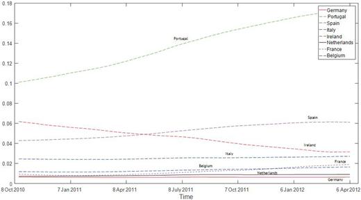
The time span has been set to one year, as assets are commonly valued on a yearly basis. The lambda and zeta values are known on a weekly basis during the testing period (2.5 years), but one-year data are needed to calculate the default probability. Thus, the default probabilities values within one year from time t have been calculated per week for 1.5 years, which include the peak of the euro debt crisis. The default probabilities can be found in Figure 6.

As can be seen in Figure 6, the default probabilities are the highest for Portugal and Spain which matches with their high CDS spread. Thus, the model reflects the implied sovereign credit risk in an adequate manner. The default probability for Portugal decreases from the beginning of 2012, which points out that Portugal is perceived by the market to take adequate steps to lower its credit risk. The default probability for Ireland is decreasing from the start of 2011, which shows that Ireland is quicker to deal with the crisis that appeared than Portugal. Germany has the lowest default probability, closely followed by The Netherlands; they can be classified as stable and safe sovereigns since their default probability values are low and stable. Belgium and France follow a similar pattern in which their values are between the relatively stable sovereigns and the more risky sovereigns. Thus, they can be classified as low risk sovereigns.

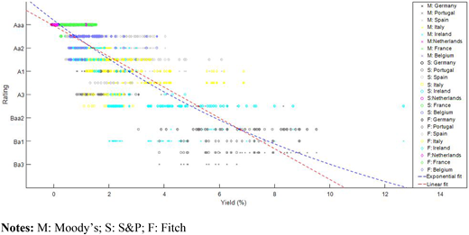
To be able to understand the relationship between the ratings assigned by the Big 3 and the market perception by the sovereign one-year maturity yield, a scatter plot has been made which can be seen in Figure 7. As there are no data available for the sovereign one-year maturity bond of Portugal and The Netherlands, the one-year yield has been calculated from the corresponding two-year maturity bond. Both a linear and exponential fit have been applied, in which the exponential fit is a closer fit compared to the linear fit. However, as we see in the plot, there is a wide range for the yield for ratings below Aa2; especially for Ba2 where yields range from 2 to 10 per cent. This shows that while the market perceives a higher level of risk, the sovereigns have the same credit rating. Hence, using bond yields alone would not be sufficient to set up a rating scheme. To complement a bond yield-based rating scheme, we can make use of our model and the default probabilities we obtain. This allows a more reliable comparison of sovereigns, since there is a quantitative metric which applies to each sovereign. We have a total of 22 buckets, each one representing a rating, which is developed as follows. As Germany is the sovereign which is used as comparison and its implied default probability is low, it is assigned the highest credit rating which is Aaa. The probability of default of the highest rating bucket is set to be maximum default probability value of Germany. When a sovereign defaults, the default probability value should have a value of 1 and it should have the lowest possible rating. We use just one rating for default, similar to Moody’s and S&P and unlike Fitch which includes three different default categories. An exponential scale has been applied to the remaining buckets. The bucket range increases as we go toward the last bucket that has the highest default probability, with 1.267 being the range multiplier ensuring that the last bucket ends with default probability of 1. The first bucket includes sovereigns with a default probability between 0 and 0.0066 per cent, and the second bucket contains sovereigns with a default probability between 0.0067 and 0.0084 per cent and so on. A nomenclature similar to Moody’s has been used for this rating scheme. The buckets can be seen in Table V.

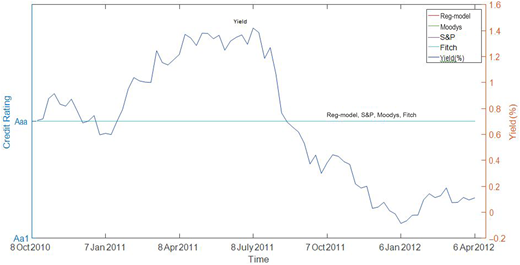
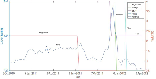
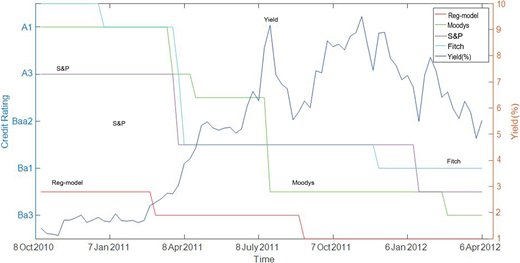
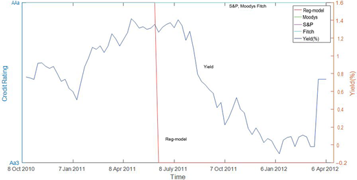
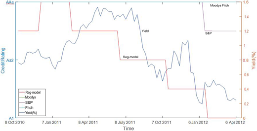
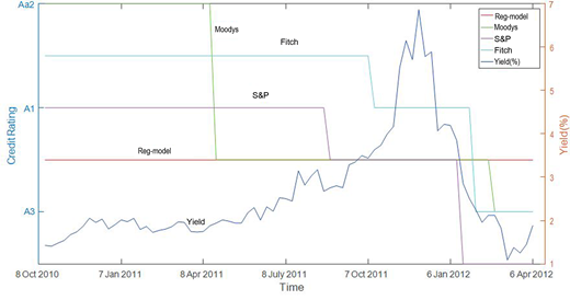
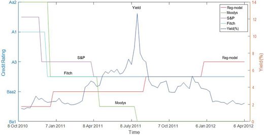
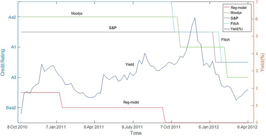
The ratings assigned by the Reg-model are compared with the ratings assigned by the Big 3, which can be seen in Figures 8-10. The sovereign one-year bond yield is also included as a benchmark. One could categorize the eight countries in three groups based upon the ratings issued by the forecasting model. The first group consists of Germany and The Netherlands, which have a low level of sovereign credit risk. The second group consists of Belgium, France and Italy, which have a small level of sovereign credit risk. The third group consists of Portugal, Spain and Ireland, which have a serious level of sovereign credit risk. The Reg-model gives Germany the highest possible rating, similar to the Big 3. Germany’s bond yields are low and have a low fluctuation which indicates that there is less implied sovereign credit risk. A similar situation can be found for The Netherlands but note that the Reg-model downgraded The Netherlands during the peak of the crisis (see Figure 11 in the Appendix).

For Belgium (Figure 9), the credit ratings issued by the Big 3 show a lag, since they start to downgrade Belgium from the start of 2012. The yield values indicate a rise in the implied sovereign credit risk midway 2011. The CDS spread indicates that there is an increase in the implied sovereign credit risk from the start of 2011. This market behavior is captured by the Reg-model and not by the credit ratings issued by Big 3. Thus, it can be concluded that the ratings issued by the Reg-model provide better insights than the ratings issued by the Big 3. The same situation applies to Italy and France (Figure 10).

For Portugal, the credit rating issued by the Reg-model follows a decreasing trend. Portugal is rated Ba3 from the beginning of 2011, indicating a serious level of sovereign credit risk. This can easily be inferred by looking at the yield values, which increase over time. The Big 3 also downgrade Portugal over time, a sharp decrease in March 2011 and again at the end of 2011. However, the CDS spread and the yield were already an early indication of high level of sovereign risk – which the Big 3 were slow to respond to. Their update at the end of 2011 was late since the yield was already quite high before. This is another example why the rating issued by the Reg-model provides better insight and faster market response compared to the Big 3. A similar situation in which Big 3 are slow to respond can also be found for Ireland and Spain.

It can be concluded that the ratings issued by the Big 3 tend to be slow to respond to market changes. The ratings are not downgraded at the moment when both the CDS spread and the sovereign bond yield increase. This is in contrast with the ratings issued by the Reg-model, which respond quicker to changes in the markets. Second, our rating scheme is a quantitative measure based on the Reg-model, allowing for a more reliable comparison between the sovereigns. This is in contrast with the rating procedure used by the Big 3, which is qualitative in nature and allows for different ratings for the same sovereign. Thus, this new procedure can be used to replace the current sovereign credit risk assessment procedure.

The credit ratings assigned to sovereigns play a crucial role in indicating the financial health of these sovereigns. The inadequacies of the ratings assigned by the Big 3 (S &P, Moody’s and Fitch) became apparent during the financial crisis of 2008. The manner in which these firms assign their ratings lacks transparency. Furthermore, the fact that these firms receive payments from the sovereigns they assess and assign ratings to leads to significant conflicts of interest issues. More crucially, as was evidenced during the financial crisis, the ratings assigned by the Big 3 are slow to respond to market changes. The current financial climate is one in which many sovereigns are vulnerable to shifts in the geopolitical landscape. Given the vital role played by sovereign credit ratings, there is an urgent need for a transparent and rigorous model that can assess the creditworthiness of a sovereign and assign ratings that are accurate and respond quickly to market changes. In this paper, we develop a framework using the CDS spreads of a sovereign to assess its creditworthiness and assign a credit rating. The framework is centered on a regression-based model to estimate the CDS spreads of sovereigns. The model adopts the notion that sovereign credit risk is composed of both systemic and idiosyncratic risk and uses historical CDS data and data on other financial and macroeconomic variables to estimate the CDS spreads of sovereigns. With these estimates, the values of the systemic and idiosyncratic risk intensity processes can be calculated. These values in turn yield estimates of the default probability of a sovereign. A ratings scale based on these estimated default probabilities is then used to assign credit ratings to the sovereigns. We tested our framework on data from eight Eurozone countries during the peak of the financial crisis. Our results show that our framework provides good estimates of CDS spreads. Furthermore, the credit ratings assigned to sovereigns using our framework and ratings scheme reflect reality better, as opposed to the credit ratings issued by the Big 3. The proposed framework is generic and readily allows for modifications in the input data. Users can adjust factors and/or add new information easily. Due to the modular nature of the framework, users can use more sophisticated models to estimate default intensities and default probabilities. For example, a non-linear regression model might be used. A dynamic factor model, with parameter estimates obtained using a Kalman Filter, in conjunction with simulation could also be used. The framework is also demonstrably accurate and responsive. The framework is also transparent in the assessment of sovereign creditworthiness and assignment of credit ratings. Furthermore, the model also allows for stress testing to be performed, a key requirement for financial models in current economic conditions.

Please note that for reasons of simplicity, the subscript i on ξ_i, a_i, b_i, c_i, and γ_i is suppressed in this appendix. There are three layers of equations for equation (8). The first layer is as follows:

The second layer of formulas is as follows:

The third and last layers are as follows:

The summary statistics of the CDS data that has been used are provided, which include the minimum, maximum, mean, median value and the standard deviation for each country for both maturities for both time periods.

Factor analyses have been conducted for each country, using the Varimax technique (which is an orthogonal rotation). This type of rotation reveals what factors are independent and are able to explain the major share of the variance. If the absolute value for a variable in a column is close to 1, then this variable can be used as a factor. These values have been shown italic font. For each country, the factor analysis has been run for four factors, but in case there is no relevant fourth factor (only low values for every variable), only the outcome of the three relevant factors is shown. Note that to determine the number of factors to be included, the Eigen values are used. If there are three variables with an Eigen value above 1, then the output includes three variables. The Eigen value explains to what extent the variable explains the variance in the data set.

The outcome of this step is then used in the regression. Only the independent factors are used in the regression analysis, and the results are shown in Tables AXIII-AXX.

For each country, a regression analysis has been conducted which uses variables chosen from the factor analysis, shown in Tables AV-AXII. These variables are chosen as they can best represent the variability in the data. We also test different lagged time series to obtain the best regression outcome. We report the following: Estimate, Standard Error, t-Statistic, Rejection value (1 p-value), the lag and the R-squared value. As can be seen, all variables have a rejection value under 1 per cent (p-value over 99 per cent) which shows that every variable is significant at a 99 per cent level. Given that there are several variables as outcome from the factor analysis, different models have been tested. The model with the highest R-square value has been reported. Note, an explanatory variable which has a high value in the factor analysis might not directly be incorporated into the final regression model.

For example, in the case of Germany, we note the independent factors to be the Oil price, the ECB interest rate, the 3-year eurobond and the EUR-RMB exchange rate from Table AV. These variables are tested with different lags and the best regression outcome is chosen, as shown in Table AXVII[³]. With multiple independent factors, we test the regression on multiple combinations of the factors and choose the best outcome.

Table AI 

Table AII 

Table AIII 

Table AIV 

Table AV 

Table AVI 

Table AVII 

Table AVIII 

Table AIX 

Table AX 

Table AXI 

Table AXII 

Table AXIII 

Table AXIV 

Table AXV 

Table AXVI 

Table AXVII 

Table AXVIII 

Table AXIX 

Table AXX 

Figure A1 

Figure A2 

Figure A3 

Figure A4 

Figure A5